Vision-Based Localization Algorithm Based
on Landmark Matching, Triangulation,
Reconstruction, and Comparison
David C. K. Yuen
, Member, IEEE,
and Bruce A. MacDonald
, Senior Member, IEEE
Abstract—Many generic position-estimation algorithms are vulnerable to ambiguity introduced by nonunique landmarks. Also, the available high-dimensional image data is not fully used when these techniques are extended to vision-based localization. This paper presents the landmark matching, triangulation, recon-struction, and comparison (LTRC) global localization algorithm, which is reasonably immune to ambiguous landmark matches. It extracts natural landmarks for the (rough) matching stage before generating the list of possible position estimates through trian-gulation. Reconstruction and comparison then rank the possible estimates. The LTRC algorithm has been implemented using an interpreted language, onto a robot equipped with a panoramic vision system. Empirical data shows remarkable improvement in accuracy when compared with the established random sample consensus method. LTRC is also robust against inaccurate map data.
Index Terms—Landmark matching, triangulation, reconstruc-tion, and comparison (LTRC), natural landmark, panoramic image, random sample consensus (RANSAC), triangulation, vision-based localization.
I. INTRODUCTION
V
ISUAL image data has the potential to disambiguate objects for localization, as it provides high resolution, and additional information such as color, texture, and shape. To compensate for accumulated navigation errors, mobile robots must use external sensors to estimate their position. Active ranging devices give direct distance measurements and have found widespread use for robot localization. However, these sensors do not provide features needed to resolve ambiguities between objects.Many animals rely on visual perception to guide their own movement. The omnidirectional vision system has evolved in many insects, including the housefly and the honey bee. It brings a very large field of view to these insects, and is valuable to their survival, as natural enemies can attack from any direction.
The design of many robot components, including the vision system, imitates the biological counterparts. Panoramic vision, which is very similar to omnidirection vision, but the zenith is not visible from the observer, has been adopted in many robotics
Manuscript received June 24, 2003; revised March 11, 2004. This paper was recommended for publication by Associate Editor K. Yoshida and Editor S. Hutchinson upon evaluation of the reviewers’ comments. This work was sup-ported in part by the Foundation for Research, Science and Technology, New Zealand, under a Top Achiever Doctoral Scholarship.
The authors are with the Department of Electrical and Computer Engineering, University of Auckland, Auckland, New Zealand (e-mail: [email protected]; [email protected]).
Digital Object Identifier 10.1109/TRO.2004.835452
studies, for example, by Yagiet al.[1] for obstacle avoidance, and by Zhuet al.[2] to train a road classification and orientation network for an autonomous land vehicle. It is worthwhile to explore techniques that assist robot localization with panoramic vision.
While most established robot-localization algorithms assume the use of direct ranging sensors, such as an ultrasonic or laser range finder, a single panoramic image does not give obstacle distance explicitly. The range information to the obstacles can only be extracted in an indirect manner. As a result, the applied localization algorithm must be amended.
A. Global Localization
Global localization, the primary interest for this paper, provides the initial position estimate for conventional robot-tracking algorithms (e.g., extended Kalman filtering) and enables the robot to identify its own position when previous odometry readings are either inaccurate or even not available (e.g., due to wheel slippage, or just after powering up). In terms of functionality, localization can be classified as global, incre-mental, or simultaneous localization and mapping (SLAM). Global localization identifies the robot position with respect to some external frame using only the current sensory data. Unlike the incremental methods, an historical position estimate is not required. The global localization application is targeted not only because it is essential to many robot navigation sys-tems, but its independence from historical position estimates also clarifies the evaluation of the proposed algorithm in the presence of nonunique landmarks.
B. Iconic Versus Feature-Based Localization
Localization methods are often classified either as iconic or feature-based. The iconic method directly compares the raw data with the map, whereas the feature-based method considers mainly the prominent features [3]. Most iconic localization al-gorithms assume the use of a range sensor and may be inap-propriate for visual information. When using an image sensor, the direct analogue for iconic localization would involve the matching of raw image pixels with a three-dimensional (3-D) lighting model of the environment. Obvious practical concerns limit the use of this approach.
A training phase can be included in the iconic method to process a reference-image database. Zhanget al.[4] trained an array of neuro-fuzzy controllers with raw omnidirectional im-ages. The robot position is then determined by choosing the most appropriate output with a situation-identification module. Cassinis and Rizzi [5] present a self-localization system that
processes the panoramic image data through both neural net-works and multiple linear regression. Their system gives low positioning error (averaging less than 10 cm), but is quite sen-sitive to errors if the robot is offset by more than about 5 from its original orientation.
Feature-based methods are often very efficient, providing that unique features can be found. Ishiguro and Tsuji [6] compare the incoming image with images captured at reference points during the exploration stage to determine the approximate robot posi-tion. The low-frequency components of the Fourier-transformed images are kept as features for comparison. The data-compres-sion method is efficient, but may cause problems when the envi-ronment is more cluttered. By triangulating the extracted land-marks from the panoramic image, Ishiguroet al. [7] estimate the relative distances between a team of robots. The method as-sumes unique and known robot appearance, which may not be valid in more general cases. Atiya and Hager [8] determine robot position with vertical image edges obtained from stereo image pairs. The observed landmark and stored map labeling problem is solved by a set-based method. Lowe [9] introduced the scale invariant feature transform (SIFT) algorithm to extract invariant features from the images. The input image is convoluted with 2-D Gaussian functions scaled by different smoothing factors. The local minima and maxima of the smoothed images are taken as the keys. Global vision localization [10] can be achieved with a random sample consensus (RANSAC) approach by matching the SIFT features between the current image and a database map.
Feature-based localization algorithms are often simpler and more reliable, especially in dynamic environments, but the presence of nonunique landmarks is the serious concern. Fea-ture-based methods can be simpler due to the lack of a training phase. It is quite common to find multiple entities of similar objects, such as a set of dining chairs, an array of partitions, or a series of doors, in the case of indoor navigation. These nonunique natural landmarks cause serious data-association problems for many generic position-estimation algorithms [11]. While unique landmarks can be introduced by the place-ment of artificial objects, the preparation, maintenance, and environment-modification requirements make them unpop-ular. Robust estimation methods, notably RANSAC [12], can tolerate outliers, “poisoned points,” or nonunique feature matches, to a certain extent. RANSAC relies on repetitive random sampling. Its performance deteriorates rapidly with an increasing proportion of nonunique matches. Markov-chain Monte Carlo expectation-maximization (MCMCEM) [13] is a promising data-association technique, which demonstrates success in solving the 3-D scene model-estimation problem from a collection of image data. It assumes that all the 3-D features are visible from all the views. Although this is a common and very reasonable assumption for computer vision, occlusion is a crucial problem that should not be overlooked in robot navigation.
C. Paper Outline
Instead of using a purely feature-based approach, we describe a novel two-stage global localization algorithm using panoramic images, which consists of a rough feature-matching stage fol-lowed by iconic-based comparison. We focus on the influence of nonunique landmarks on vision-based localization, which
is a particular concern in a cluttered indoor environment. The image representation is reconstructed to remove the perspec-tive viewing effect before comparison. The proposed method, landmark matching, triangulation, reconstruction, and compar-ison (LTRC), works well when compared with the established RANSAC robust estimation technique. We believe the direct comparison between the high-dimension image representations of the current and reference images, rather than between the low-dimension position estimates, assists the matching between corresponding landmarks, and thus improves the overall local-ization performance. Tests have been carried out in a cluttered office, where the influences from both similar objects and oc-clusion are strong.
The data-association problem caused by the presence of nonunique landmarks is illustrated further in Section II. Sec-tion III outlines our LTRC vision-based localizaSec-tion approach. To link the vision input to existing map data, some images around the robot workspace must be captured. The reasons for the selection of the generalized Voronoi vertices as the refer-ence image-capturing sites are also discussed. The empirical results are shown in Section V, and the paper is concluded in Section VI.
II. PROBLEMANALYSIS
In this paper, the coordinates and the heading direction of the robot are the only state variables of interest,
. For a panoramic image, the map position of the landmark and the viewing angle of it from the ob-server position can be defined as an ordered observation pair . A minimum of only three observation pairs are re-quired to estimate the robot position, and the amount of obser-vation data available is often more than the minimum required to solve the triangulation equation system.
A number of generic estimation procedures [11], including least-squares (LS), maximum-likelihood estimators, RANSAC, and various clustering techniques, have been adopted in com-puter vision to handle the redundant information. However, it is often difficult to ensure the nonambiguous association amongst all the observation pairs. Not many generic estimation methods can handle this type of nonunique matching error.
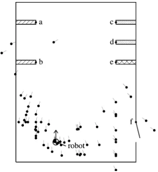
When natural landmarks are being extracted, it is quite common to find several similar objects. Fig. 1 shows a room with only six natural landmarks . Nonunique landmarks
and have pattern
while and have pattern
Since the image regions around these landmarks are very sim-ilar, it is difficult to distinguish them. Therefore, if a landmark with pattern
sim-Fig. 1. Multiple position estimates. Dots represent position estimates, and the short line segments, the direction. Only about half of the 120 estimates are shown, as the remainders are outside the region.
ilarity between landmarks and . In general, observation pairs can be formed from a set of similar landmarks. Suppose the robot can see all six landmarks, the total number of observa-tion pairs is . The robot position is esti-mated by triangulating any three arbitrarily chosen observation pairs. A maximum of possible position estimates (see Fig. 1) will have to be checked, whereas the search space is only if the landmarks are unique.
Most generic estimation procedures are vulnerable to the sys-tematic error introduced by the erroneous observation pairs. It is well known that the LS method is accurate only if the data error is normally distributed [14]. Clustering methods are also likely to fail. As illustrated in Fig. 1, the cluster associated with the actual robot position does not have a significantly larger mem-bership when compared with other ones.
RANSAC is a robust estimation technique. While it has a greater tolerance toward data inconsistency, a high proportion of poisoned points renders the method inefficient. A small con-sensus data set is randomly selected, which can be any three observed landmarks in the case of 2-D global localization. A position estimate is evaluated from this consensus data set. Ad-ditional data points (landmarks) are added if they give consis-tent position estimates with the existing consensus data set. The solution is accepted when the consensus set grows to a prede-termined size . If no acceptable solution is found, the process will be reinitialized with a different random consensus set until a maximum trial number is reached. For a fixed rate of success, the expected trial number is
where is the proportion of outliers [12]. All the erroneous ob-servation pairs introduced in Fig. 1 are considered as poisoned points, which renders RANSAC inefficient. More importantly, some false solutions generated from multiple erroneous obser-vation pairs can form a fairly large consensus set, and thus make the estimation more liable to errors.
Although RANSAC is the most reliable method described, it fails to use all the available vision data. Trying to resolve the ambiguity from only the low-dimension position estimate is dif-ficult. Therefore, a reconstruction stage should be introduced to
remove the perspective effect, so that the high-dimension cur-rent image input can be compared with the reference data.
III. LTRC ALGORITHM
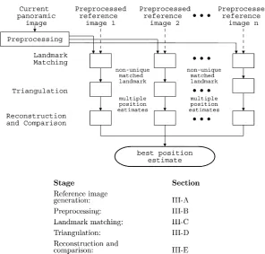
The preprocessing, LTRC stages are the main components of the LTRC algorithm (Fig. 2); details are in subsections fol-lowing the summary below. The combination of feature then iconic localization is the distinguishing characteristic. LTRC as-sumes the availability of a simple map of the workspace, and a set of reference images previously taken from known positions in the environment. It accepts the current panoramic view from the robot as the only input, and ignores any historical position estimates.
First, reference images are generated and preprocessed (Al-gorithm 1). To reduce image computation, a representative 1-D color scalar array is generated for each image during prepro-cessing. Natural landmarks are also extracted at this stage. Most indoor scenes are filled with close-range objects, and perspec-tive viewing effects are too significant to be ignored. The vertical image edges are thus extracted as the natural landmarks, due to their invariance to perspective changes. Depending on the op-erating environment, other prominent image features, such as SIFT [9], corners, and regions with special pattern or texture, can also be selected as features.
Algorithm 1Reference Image Preparation
Generate generalized line Voronoi diagram (GVD) from floor plan
for allGVD verticesdo Capture reference image Compute scalar array end for
Once the current image is preprocessed, the land-mark-matching stage identifies a short list of consecutive landmark matches (Algorithm 2). Instead of being sampled randomly as in RANSAC, observed natural landmarks are matched with those landmarks extracted from each of the reference images. The corresponding points are triangulated to estimate the current robot position.
However, there may be erroneous estimates:
• images of such natural landmarks are not unique; there may be many similar images of many similar object edges; • not all object edges will form image edges; for example,
when an object is next to another one of similar color; • not all image edges are projections of object edges; for
ex-ample, some image edges are caused by stripes on objects; • when an object is occluded, its edge in the image may
appear in the wrong place;
• in nearly every robot environment, there is more than one reference site; some of these may not match well to the current view.
[image:3.594.85.244.64.237.2]Fig. 2. Overview of the LTRC localization system.
Algorithm 2LTRC Localization Capture current image
Compute scalar array
for all do
Find matched-feature triplets between and
for all do
Get observation pairs , , from
end for end for
A. Reference-Image Generation
More than one reference image is taken, since most robot en-vironments contain both convex and nonconvex corners, which may block the view of an observer from some of the locations. During the map-preparation stage, the reference images are taken from strategic positions around the workspace. The exact locations and camera orientations of the reference sites are recorded. The reference images will be compared with the current captured image to identify the corresponding landmarks at the position estimation stage.
The reference surveying sites should be selected such that the combined view from these sites provides a complete coverage of the workspace. That is, to ensure the existence of at least one reference image that can be reconstructed to match any single possible view captured from the workspace
Reconstruct (1)
where , can be any valid position in the workspace and . Due to the dynamic nature of the environment, the criterion may have to be relaxed, in reality. Nevertheless, the system should at least place surveying sites in neighboring re-gions where the visibility toward any major object is different. In addition to full-view coverage, the reference sites should ide-ally be situated far away from obstacles to improve the use of the panoramic view. The total number of reference sites should also be kept to a minimum to reduce site preparation and main-tenance.
A number of site-selection techniques were found lacking, such as uniform sampling, the art-gallery solution, and view-in-variant partitioning. The placement of reference sites on a uniform grid is the simplest solution, but full coverage results in too many redundant sites. The art-gallery problem involves the assignment of vertex guards such that the entire polygonal workspace is visible by at least one of the guards. The required number of sites is less than for a simple polygon with holes, where is the number of object edges [15]. However, guarding posts are placed at either the corner or the edge positions, where the neighboring boundaries unavoidably block a significant proportion of the panoramic view. The view-invariant region (VIR) polygon partitioning algorithm introduced by Simsarianet al. [16] decomposes the map into a set of disjoint VIRs, each of which is characterized by the map or obstacle edges that are visible from points within it. Characteristic points such as centroids are selected within the VIRs to guarantee complete view coverage and provide a certain clearance from obstacles. However, this method creates many more reference sites than the former one, e.g. for a simple polygon with holes.
Fig. 3. GVD for a typical room.
, which outlines the workspace boundary and the obstacles. The GVD can be defined as the tessellation formed by the boundary set of the Voronoi polygons , i.e.,
(2) where is the Euclidean distance from point to a member of the generator set [17].
GVD vertices have a number of desirable geometric proper-ties which make them a good choice for the placement of ref-erence sites. The view coverage is almost complete if the sur-veying sites are located at these vertices1 (Fig. 3). The GVD
vertices are equidistant from at least three or more generator ob-jects. Since the vertices are kept well away from obstacles, the panoramic view captured will be more representative. The pos-sibility of sharing the computation with other navigation mod-ules, e.g., path planning [18], [19] or mapping [20], [21], further supports our proposed selection. For a room with modest com-plexity , the required number of reference sites is reduced by at least an order of magnitude if GVD vertices are selected instead of the VIR centroids (Fig. 4).
For environments with a lot of free space, e.g., inside a large sports stadium, distant landmark features may appear to be small. Although the proposed method mainly considers cluttered environments, extra reference sites can be added along the long Voronoi edges to extend its application. We do not want reference sites at corners and edges of objects, as these locations can be difficult to access. Besides, the view can be highly distorted if the camera is placed very close to an obstacle.
While this work generated the GVD from ana priori floor plan and the robot was driven manually to the reference GVD vertex site during the preparation stage, it is possible to make the operation fully autonomous by building the GVD incrementally with the onboard range-finding sensors [22].
B. Preprocessing
The current and reference panoramic images are generated by stitching together single 24-b color snapshots from a Sony XC-999 camera mounted on a rotating platform. Since our pro-posed algorithm does not really rely on high-resolution input,
[image:5.594.303.551.65.192.2]1Although using GVD vertices can achieve full-view coverage in most real-world environments, theoretically, there are degenerated cases where the visib-lity is more limited.
Fig. 4. Required number of reference sites for maps with different complexity, wherenis defined as the number of object edges. Among the 23 sample maps, some have up to 12 holes.
the raw panoramic images of 1920 240 24-b color pixels are trimmed to 1920 80 along the central line of the vertical axis, then downsampled to 192 80 with a median filter. A lower res-olution design, such as a conical or parabolic mirror, could be substituted for the rotational panoramic camera.
The color vector for each pixel is converted to a representative color scalar. The best choice of 1-D color scalar is dependent on the color distribution of objects in the workspace. Our previous paper [23] found little difference in further localization stages when using three different color scalars: the intensity, hue, and modified hue index (MHI).2In this paper, we also examined all
three indexes, but only report the MHI results for simplicity. Vertical edges are extracted by thresholding the resulting image after processing through the Sobel vertical operator. Only those edges longer than 40 pixels, i.e., half the height of the trimmed image, are kept as natural landmarks [Fig. 5(c)]. They also serve as boundaries to separate the supposedly uniform image regions, known as tokens. Each token may correspond to a separated object or a portion of a single object (e.g., a wall painted with different colors on opposite ends). The median color scalar of the left and right token is calculated as a signature for each landmark to facilitate matching. For example, the landmark corresponding to the edge formed be-tween unpainted wood and a concrete wall can be characterized by the brown-gray color scalar pair.
A more compact image representation is needed to improve the efficiency of image comparison. A 1-D color scalar array [Fig. 5(b)] is generated for the current image or the indi-vidual references images , by evaluating the median color scalar in a column-by-column manner.
C. Landmark Matching
A pair of landmarks is said to be similar if the difference be-tween their individual signatures (median color scalars) is
suf-2MHI is essentially the hue component of hue–saturation–value (HSV) color space with provisions for colors with low saturation values (white, grey, or black)
MHI =
0120:0 5 (black)
090:0 < 5 & 5 < 90 (grey) 060:0 < 5 & > 90 (white)
otherwise
(3)
Fig. 5. Preprocessing stage. (a) Raw panoramic image. (b) Color scalar array (S). (c) The extracted landmarks (the thick vertical lines) and their corresponding signatures (taken as the median MHI color scale of the pixels bounded by two neighboring landmarks).
Fig. 6. Position estimation process. (a) Simple room map shows the current robot position, = (x ; y ; ), and one of the reference sites = (x ; y ; ). (b) 1-D color scalar array for the current and reference view. A sample pair of corresponding landmarks (landmarkj) is highlighted by a solid triangle. (c) Looking up the map position of landmarkjby drawing an extension line from the reference site i along the direction of . (d) Triangulation.
ficiently small. Expecting a consecutive match along the entire landmark sequence is not realistic, due to partial occlusion and slight environmental changes. On the other hand, nonunique landmarks are a common occurrence. To reduce the rate of mis-matching, only landmark sequences with at least three consec-utive matched features are considered.
The landmark signature list of the current image is compared with that generated from each of the reference images. The op-eration often finds multiple sets of consecutive matched land-marks. Robot position estimates are obtained from the triangu-lation of these matched landmark sets, and the best one is se-lected during the reconstruction and comparison stage (see Sec-tion III-E).
The landmark-matching process is illustrated in Fig. 6. After the identification of the consecutive matched landmarks from the color scalar arrays [Fig. 6(b)], the corresponding ob-served angles to these landmarks are recorded. Since the color
Fig. 7. Nomenclature for the triangulation equations.
scalar arrays are essentially vertically compressed panoramic images, the landmark location on them is proportional to the ob-served angle. The physical positions of landmarks of the map are deduced by drawing an extension line from the reference site, as in Fig. 6(c). The intersection of this line with the nearest obstacle gives the map position, and can form an observation pair
. Triangulation of the robot position requires the recognition of at least three matched landmarks between the ref-erence and current images. For a consecutive matched-feature triplet, the first three observation pairs are taken as the inputs for the triangulation equations [Fig. 6(d)].
D. Triangulation
The general triangulation equations when using projective ge-ometry [14] are shown in (4) and (5). The parameters are de-scribed in Fig. 7
(4)
(5) where
(6) For our current panoramic camera settings, the geometry can be simplified. Capturing an image is equivalent to stitching the vertical strips in the middle of each image captured when ro-tating the camera along its axis. In other words, the
[image:6.594.51.279.316.476.2]that and should be set to and 0, respectively. As the panoramic images are collapsed to 1-D color scalar arrays after preprocessing, (5) can be ignored. Since the zeroing position of the panoramic camera is linked to the robot heading direc-tion and the bearing system adopted is different, is substituted with . Equation (4) is simplified to
(7) The robot position and heading direction are found by solving a set of triangulation equations (7) using a fail-safe ver-sion of the Newton–Raphson root-finding algorithm.
E. Reconstruction and Comparison
Since our algorithm assumes no previous knowledge of the robot position, the estimation procedure must be repeated for each of the reference views, and reconstruction is used to select the best estimate. As explained in Section II, multiple matches may be obtained, even if only one reference site is considered.
Perspective distortion must be corrected, otherwise, direct comparison between two color scalar arrays provides little hint regarding the similarity between the regions. The reference image under examination is reconstructed as if it is now taken at the suggested position. If the estimate is, in fact, close to the correct robot position, the current color scalar array will be very similar to the reference view . Thus, and
can be compared directly.
The reference color array shown in Fig. 6(b) is arranged in compass order. A ray is drawn from the reference site to the viewing direction of each token boundary on the map. The co-ordinate of the nearest intersection from each ray is recorded and mapped to a corresponding value on to give . The reconstructed array is calculated from rectan-gular mapping for the reference color scalar array using (8)–(10) before converting back to the polar form
(8)
(9) (10) A similarity score is assigned when comparing with . Two different indexes,%similarityand correlation coeffi-cient, are examined. The%similarityis taken as the length ratio of similar bands between and . The reference color scalar array is first subtracted from that of the captured one. The bands between the two scalar arrays are assumed to be similar if their absolute difference is less than 20 color scalar units. The reconstruction and comparison process is repeated for each po-sition estimate.
The estimate which leads to the highest similarity score is re-garded as the solution of the localization algorithm. Erroneous estimates caused by landmark misclassification, local occlusion, nonunique matching, etc., are usually rejected due to low simi-larity scores.
IV. RANSAC ALGORITHM
The performance of the proposed LTRC algorithm (Algo-rithm 2) is compared with the established RANSAC algo(Algo-rithm
(Algorithms 3 and 4) in Section V. To enable a fair comparison, both of them share the same preparation procedure for reference images (Algorithm 1). The differences between various auxil-iary procedures, e.g., color scalar array and landmark matching, are also kept to a minimum.
Algorithm 3RANSAC Localization Capture current image
Compute scalar array for all do
Find matched feature triplets between and
for all do
Add any unique observation pairs to end for
; Algorithm 4
end for
Similar to LTRC, consecutive matched-feature triplets are identified between the current image and the reference image under examination. Unique observation pairs, which indicate the position of the feature and its orientation from the cur-rent viewing point, are added to set . The largest consensus set is then found using a standard RANSAC implementation [12], as indicated in Algorithm 4. By triangulating the members in , a number of possible robot positions are obtained. The current robot position is taken as the centroid of these possible positions.
If the best reference site is not known, a similarity score will be evaluated when the current scalar array is compared with each reference . Again, the estimate which leads to the highest similarity score is regarded as the solution of the localization algorithm.
Algorithm 4Find the largest consensus set (RANSAC)
for do
Draw three members randomly from to form
while do
Draw from and
if then
end if end while
if then
break end if end for
Fig. 8. View of the testing room.
to set if the triangulated robot positions are consistent. The calculation is repeated until either the size of the consensus set becomes larger than or the maximum number of iter-ations is reached.
A fundamental difference can be identified between the algo-rithms, which is even more clear if we consider the simpler case where the best reference site is known. For LTRC, a similarity score is generated by comparing the reconstructed reference scalar array with the current one. It is a high-dimension com-parison based on the observation. On the contrary, RANSAC is limited by the consensus set formation for the observation pairs. The consistency between the triangulated positions becomes the decision criterion. It is a low-dimension comparison based on the state estimates. The implications of the difference are clearly shown in the next section.
V. RESULTS
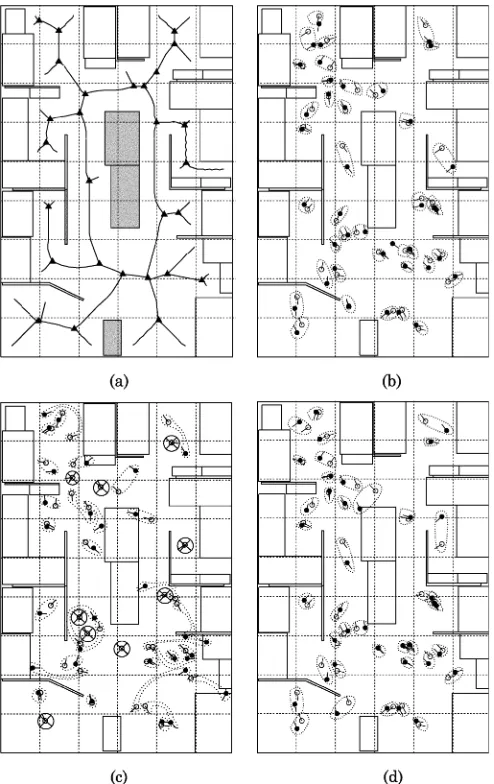
Tests were carried out with a B21r robot in a heavily cluttered 6.0 9.0 m student office (Fig. 8), which was partitioned into a number of similar cubicles. Part of the room was influenced by ambient lighting, and tests had been run both day and night. The room consists of 28 GVD vertices [Fig. 9(a)] and 5994 VIRs. The choice of GVD vertices as reference sites is the only prac-tical solution to keep the number of sites to a manageable value. Images were taken from a number of randomly chosen sites during testing. The ground truth position is measured by a tape to within the nearest 10 mm. The captured panoramic images were preprocessed before being further examined with different localization schemes. An average of 16 landmarks, ranging from 9 to 25, were extracted per panoramic image. Only 55% of those are unique landmarks. The proximity of obstacles in a heavily cluttered environment also amplifies the perspective viewing problems. Both conditions make the environment difficult for the robot to localize in.
The closest visible GVD vertex to a particular sampling point is defined as the best reference site. We first examine the simpler case in Section V-A, in which the best reference site is known. Then, the more difficult case is examined in Section V-C, in which the best reference site is not known.
Fig. 9. Room map with reference sites. (b)–(d) Actual and estimated sample positions under various localization conditions. Both (b) and (d) show results when%similarityis used as the similarity score for LTRC. (—actual position, —estimated position; each sample and its associated estimate is paired by a dotted curve. If the positioning error is greater than 1.6 m, the estimate will not be shown with the sample marked by asymbol. (a) Room map with GVD outline ( —reference site). (b) LTRC results when best reference is known. (c) RANSAC results when best reference is known. (d) LTRC results when best reference is not known.
A. Best Reference Site is Known
When%similarity between and is selected as the similarity score, the LTRC localization algorithm gives very satisfactory performance [Fig. 9(b)]. The mean and median positioning errors are less than 0.20 and 0.19 m, respectively. Assuming an arbitrary robot heading angle effectively introduces an extra dimension for the vision-based localization. Many solution architectures, including multiple linear regres-sion and neural networks [5], do not scale well for this change. For LTRC, the mean and median orientation localization errors are less than 0.055 and 0.034 rad ( and 2.0 ), on par with the accuracy of many digital compasses. The matched landmark locations provide a good estimate for the rotation angle and greatly improve the results.
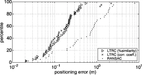
[image:8.594.57.275.63.257.2]er-Fig. 10. Error distribution for various localization conditions when best reference is known.
rors are smaller. However, for the worst 15% of samples, %sim-ilaritygives consistently fewer errors. The correlation operation highlights the trend differences, which may give a misleadingly high similarity score when two color scalar arrays share sim-ilar trends but with vastly different color, e.g., consecutive red MHI versus consecutive yellow MHI regions. For similar reasons, it penalizes some combinations of color mismatches more heavily than others. These problems become more apparent when localization error and the mismatching rate are high, and this explains the deterioration in performance.
RANSAC performs badly when compared with LTRC. Due to the stochastic nature of RANSAC, that position-estimation procedure was rerun eight times. The median positioning and orientation localization errors range from 0.52 to 0.88 m and 0.20 to 0.61 rad, respectively; all are at least three times worse than LTRC. Fig. 9(c) shows the estimated errors taken from one of the particular runs (with median localization error of 0.76 m). The same set of data is also plotted on Fig. 10. While a fairly large consensus set can be found for most samples, a signifi-cant proportion of them ( 25%) still have a positioning error of larger than 1.6 m. The ambiguity is difficult to resolve without using the extra information contained in the images.
The algorithms are implemented in Python, an interpreted language, and time of execution is recorded for both LTRC and RANSAC experiments. On average, RANSAC takes 108.5 s, whereas LTRC takes 2.9 s to localize when tested with an Athlon XP1600 PC. To form a consensus set, Sec-tion II explains that RANSAC needs to sample a lot more combinations from the observation pairs when nonunique landmarks are present. The expected number of sampling steps
required is in . Based on the
assumption of 37.5% of nonunique landmarks with a consensus
set size , would be 615 times at a
90% confidence level. In comparison, the consecutive land-mark-matching step limits the estimates that require testing in LTRC. The panoramic images collected have an average of 16 landmarks. The number of consecutive landmark matches would be quite modest.
B. Inaccurate Map Data
[image:9.594.301.551.65.195.2]LTRC performs robustly when a few objects, shown in gray in Fig. 9(a), are removed from the map before running the test again. A good localization algorithm should be immune to small discrepancies in thea priorimap. The results are compared in Fig. 11. RANSAC is a well-known robust estimation method. Its
Fig. 11. Error distribution when the map given is incomplete.
Fig. 12. Error distribution when the best reference site is unknown.
median increases from 0.76 to 0.92 m, which is less than 25%. LTRC is not affected much by the data removal, either. While the position estimation significantly deteriorates in the worst cases (about 10%), its median increases by only 0.03–0.22 m. The consecutive landmark-matching stage accepts good partial matches, and thus improves the robustness.
C. Best Reference Site is Unknown
The LTRC method also performed well in a workspace with multiple reference sites. The algorithm is basically the same as the previous case, except the LTRC calculation is repeated be-tween the current view and each of the references.%similarity is used as the similarity score. The results are shown in Fig. 9(d) and Fig. 12. The mean and median localization errors are 0.21 and 0.17 m, respectively, fairly close to the simpler case where the closest visible GVD vertex is known. The magnitude of lo-calization error is not much affected by the change.
VI. CONCLUSION
[image:9.594.41.294.66.196.2] [image:9.594.303.551.230.358.2]LTRC has also been extended to maps with multiple reference sites.
Experimental results show practical improvement of LTRC over the established RANSAC robust estimation method. The landmark-extraction stage efficiently reduces the search space, while allowing a certain tolerance to incomplete matching. In addition, the LTRC algorithm does not simply discard the visual information after the natural landmark-extraction stage. It gen-erates a similarity score according to the high-dimension restructed image representation, whereas RANSAC finds a con-sistent set from the low-dimension position estimate. For these two reasons, LTRC improves the localization performance in the presence of similar objects.
Different heuristics, such as identifying the most probable reference position by statistical means, can be introduced to sim-plify the calculation for the multiple reference sites case. Sim-ilarly, landmark extraction also benefits by the use of more so-phisticated image-processing procedures. These illustrate some of the directions for future studies.
REFERENCES
[1] Y. Yagi, Y. Nishizawa, and M. Yachida, “Map-based navigation for a mobile robot with omnidirectional image sensor COPIS,”IEEE Trans. Robot. Autom., vol. 11, pp. 634–647, Oct. 1995.
[2] Z. Zhu, S. Yang, G. Xu, X. Lin, and D. Shi, “Fast road classification and orientation estimation using omni-view images and neural networks,”
IEEE Trans. Image Process., vol. 7, pp. 1182–1197, Aug. 1998. [3] R. R. Murphy,Introduction to AI Robotics. Cambridge, MA: MIT
Press, 2000, p. 415.
[4] J. Zhang, A. Knoll, and V. Schwert, “Situated neuro-fuzzy control for vision-based robot localization,”Robot. Auton. Syst., vol. 28, pp. 71–82, 1999.
[5] A. Rizzi and R. Cassinis, “A robot self-localization system based on omnidirectional color images,”Robot. Auton. Syst., vol. 30, pp. 23–38, 2001.
[6] H. Ishiguro and S. Tsuji, “Image-based memory of environment,” in
Proc. IEEE/RSJ Int. Conf. Intell. Robots Syst., vol. 2, 1996, pp. 634–639. [7] H. Ishiguro, K. Kato, and M. Barth, “Identifying and localizing robots with omnidirectional vision sensors,” in Panoramic Vision: Sensors, Theory, and Application, R. Benosman and S. B. Kang, Eds. New York: Springer-Verlag, 2001, pp. 376–391.
[8] S. Atiya and G. D. Hager, “Real-time vision-based robot localization,”
IEEE Trans. Robot. Autom., vol. 9, pp. 785–800, Dec. 1993.
[9] D. G. Lowe, “Object recognition from local scale-invariant features,” in
Proc. Int. Conf. Computer Vision, Corfu, Greece, 1999, pp. 1150–1157. [10] S. Se, D. G. Lowe, and J. Little, “Global localization using distinctive vi-sual features,” inProc. Int. Conf. Intell. Robots Syst., Lausanne, Switzer-land, 2002, pp. 226–231.
[11] A. Gruen and T. Huang, Eds.,Calibration and Orientation of Cameras in Computer Vision. New York: Springer, 2001, pp. 63–94. [12] M. A. Fischler and R. C. Bolles, “Random sample consensus: A
para-digm for model fitting with applications to image analysis and automated cartography,”Commun. ACM, vol. 24, no. 6, pp. 381–395, 1981.
[13] F. Dellaert, S. M. Seitz, C. E. Thorpe, and S. Thrun, “EM, MCMC, and chain flipping for structure from motion with unknown correspondence,”
Machine Learning, vol. 50, pp. 45–71, 2003.
[14] C. C. Slama, Manual of Photogrammetry, 4th ed. Bethesda, MD: Amer. Soc. Photogrammetry, Remote Sensing, 1980.
[15] J. O’Rourke,Art Gallery Theorems and Algorithms. Cambridge, U.K.: Oxford Univ. Press, 1987, p. 126.
[16] K. T. Simsarian, T. J. Olson, and N. Nandhakumar, “View-invariant re-gions and mobile robot self-localization,”IEEE Trans. Robot. Autom., vol. 12, pp. 810–816, Oct. 1996.
[17] A. Okabe, B. Boots, K. Sugihara, and S. N. Chiu,Spatial Tessellations: Concepts and Applications of Voronoi Diagrams, 2nd ed. New York: Wiley, 2000, pp. 169–178.
[18] N. S. Rao, N. Stoltzfus, and S. Iyengar, “A “retraction” method for learned navigation in unknown terrains for a circular robot,”IEEE Trans. Robot. Autom., vol. 7, pp. 699–707, Oct. 1991.
[19] O. Takahashi and R. Schilling, “Motion planning in a plane using generalized Voronoi diagram,”IEEE Trans. Robot. Autom., vol. 5, pp. 143–150, Apr. 1989.
[20] S. Thrun, “Learning metric-topological maps for indoor mobile robot navigation,”Artif. Intell., vol. 99, pp. 21–71, 1998.
[21] H. Choset and K. Nagatani, “Topological simultaneous localization and mapping (SLAM): Toward exact localization without explicit localiza-tion,”IEEE Trans. Robot. Autom., vol. 17, pp. 125–137, Apr. 2001. [22] I. Konukseven and H. Choset, “Mobile robot navigation: Implementing
the GVG in the presence of sharp corners,” inProc. IEEE/RSJ Int. Conf. Intell. Robots Syst., vol. 3, 1997, pp. 1218–1223.
[23] D. C. Yuen and B. A. MacDonald, “Natural landmark based localiza-tion system using panoramic images,” inProc. IEEE Int. Conf. Robot. Autom., vol. 1, Washington, DC, May 2002, pp. 915–920.
David C. K. Yuen(S’01–M’05) received the B.E. degree (1st class) in chemical engineering and the M.E. degree in electrical and electronic engineering in 1997 and 1999, respectively, both from the Univer-sity of Auckland, Auckland, New Zealand, where he is currently working toward the Ph.D degree in robot localization in the Department of Electrical and Com-puter Engineering.
His research interests include robotics and control systems.
Bruce A. MacDonald (S’77–M’79–SM’04) re-ceived the B.E. (1st class) and Ph.D. degrees from the Electrical Engineering Department, University of Canterbury, Christchurch, New Zealand.