Fast Adaptive Augmented Lagrangian Digital Image Correlation

(1)

Correlation

Thesis by

Jin Yang

In Partial Fulfillment of the Requirements for the Degree of

Doctor of Philosophy

CALIFORNIA INSTITUTE OF TECHNOLOGY Pasadena, California

2019

(2)

Jin Yang

ORCID: 0000-0002-5967-980X

(3)

ACKNOWLEDGEMENTS

First, I would like to express my deep appreciation for my advisor, Prof. Kaushik Bhattacharya, for giving me five years’ mentorship and support. I am so lucky to be a student of Kaushik, who is open-minded, patient, kind, and intelligent. I learned a lot from him about doing research, finding good problems, and focusing on the most important goals not only in academia; I also learned lots of tips from him in my personal life about how to be a good husband, a good friend, and a good father in the future. I am very thankful to my chair of committee, Prof. Guruswami Ravichandran, for his guidance and suggestions throughout my research. Ravi is a knowledgeable, optimistic and patient person. He always gives me encouragement on my research progress and helps me build confidence. I would like to thank Prof. Jose Andrade and Prof. Jean-Philippe Avouac for serving on my committee and providing valuable feedback on my work.

I would like to thank Prof. Michael Ortiz, Prof. Rodney Clifton, Prof. Dennis Kochmann, Prof. Ares J. Rosakis, and many other brilliant professors at Caltech who taught me math and solids courses. I would like to thank Prof. Nadia Lapusta, who let me TA and have teaching experience in her classes. I would like to thank Dr. Michael Mello and Dr. Vito Rubino for insightful discussions about my research. I also would like to thank our experienced engineer, Petros Arakelian, for helping me set up experimental equipment.

I would like to thank my friends and colleagues in Kaushik-Ravi group: Paul Mazur, Hao Zhou, Chun-Jen Hsueh, Dingyi, Victoria(Tori) Lee, Ying Shi Teh, Kevin Korner, Sai Sharan Injeti, Swarnava Ghosh, Stella Brach, Louisa Avellar, Paul Plucinsky, Gal Shmuel, Aaron Stebner, Likun Tan, Xin(Cindy) Wang, Lincoln Collins, Srivatsan Hulikal Sampath Kumaran, Vinamra Agrawal, Mauricio Ponga, M. Zubaer Hossain, Andrew W. Richards, Ha T. Giang, Jocob Notbohm, Noy Cohen and Ruobing Bai. Thank you all for your help and insightful discussions throughout my PhD years.

(4)

I would like to thank all my friends from Caltech MCE, CaltechC, and CaltechY. I had a lot of good times with you guys, especially Wei Mao, Zheng Li, Yanan Sui, Feng Bi, Jiaming Li, Lucy Yin, John Pang, Yuanlong Hunag, Xiaobing Xiong, Luis Phillipe C Tosi, John K. (Kenny) Buyco, Kazuki Maeda, Nicholas Burali, Nikola Z. Georgiev, Brandon Runnels, Kimberly A. Mac Donald, Tomoyuki Oniyama, Christian Kettenbeil, Liuchi Li, Wen Chen, Cheng Li, Wen Yan, Charles S. (Stan) Wojnar, Zachary Erickson and Jacob Lin.

(5)

ABSTRACT

Digital image correlation (DIC) is a powerful experimental technique for measuring full-field displacement and strain. The basic idea of the method is to compare images of an object decorated with a speckle pattern before and after deformation in order to compute the displacement and strain fields. Local Subset DIC and finite element-based Global DIC are two widely used image matching methods; however there are some drawbacks to these methods. In Local Subset DIC, the computed displacement field may not satisfy compatibility, and the deformation gradient may be noisy, especially when the subset size is small. Global DIC incorporates displacement compatibility, but can be computationally expensive. In this thesis, we propose a new method, the augmented-Lagrangian digital image correlation (ALDIC), that combines the advantages of both the local (fast and in parallel) and global (compatible) methods. We demonstrate that ALDIC has higher accuracy and behaves more robustly compared to both Local Subset DIC and Global DIC.

DIC requires a large number of high resolution images, which imposes significant needs on data storage and transmission. We combined DIC algorithms with image compression techniques and show that it is possible to obtain accurate displace-ment and strain fields with only 5 % of the original image size. We studied two compression techniques (discrete cosine transform (DCT) and wavelet transform), and three DIC algorithms (Local Subset DIC, Global DIC, and our newly proposed augmented Lagrangian DIC (ALDIC)). We found the Local Subset DIC leads to the largest errors and ALDIC to the smallest when compressed images are used. We also found wavelet-based image compression introduces less error compared to DCT image compression.

(6)

PUBLISHED CONTENT AND CONTRIBUTIONS

[1] J Yang and K Bhattacharya. “Fast adaptive global digital image correlation”. In:Advancement of Optical Methods & Digital Image Correlation in Exper-imental Mechanics. Vol. 3. 2019. Chap. 7. doi: https://doi.org/10. 1007/978-3-319-97481-1_7_.

J. Yang derived the main result of this paper.

[2] J Yang and K Bhattacharya. “Augmented Lagrangian digital image correla-tion”. In:Experimental Mechanics. Under review(2018).

[3] J Yang and K Bhattacharya. “Combining image compression with digital image correlation”. In:Experimental Mechanics. Under review(2018). J. Yang derived the main result of this paper.

[4] J Yang and K Bhattacharya. “Efficient FFT-based digital image correlation”. In:To be submitted(2018).

[5] J Yang and K Bhattacharya. “Multigrid adaptive mesh digital image correla-tion”. In:To be submitted(2018).

[6] AP Stebner et al. “Transformation strains and temperatures of a nickel-titanium-hafnium high temperature shape memory alloy”. In:Acta Materialia 76 (2014), pp. 40–53. doi: https : / / doi . org / 10 . 1016 / j . actamat . 2014 . 04 . 071_{. url:} http : / / www . sciencedirect . com / science / article/pii/S1359645414003346_.

(7)

LIST OF ILLUSTRATIONS

Number Page

2.1 DIC reference imagef(X)deforms into deformed imageg(y(X)). . 6 2.2 The change of variables involved in the IC-GN update. . . 10 2.3 Comparison between Local Subset DIC and Global DIC. . . 11 3.1 Convergence of the ALDIC method for the SEM 2D-DIC synthetic

images, Sample 1 representing translation. . . 23 3.2 Comparison of RMS error in displacement (a) and strain (b) computed

with the three methods for the synthetic images in the SEM 2D-DIC, Sample 1 or translation. . . 24 3.3 Exact horizontalx-displacement and strainexx field associated with

Sample 14 images L1, L3, and L5. . . 24 3.4 Convergence check of ALDIC algorithm in Sample 14 L1, L3, and L5. 26 3.5 The horizontal displacement (u) obtained using the three methods

from the synthetic images of SEM 2D-DIC Sample 14: L1, L3, and L5. . . 27 3.6 The horizontal longitudinal strain (exx) obtained using the three

meth-ods from the synthetic images of SEM 2D-DIC Sample 14: L1, L3, and L5. . . 28 3.7 Heterogeneous specimen used for the third case study. (a) Front view

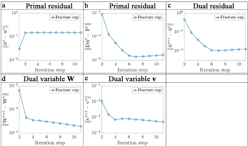
of designed fracture specimen with brick architecture, where the box area will be captured using a CCD camera. (b) A speckle pattern is applied using white spray paint onto the surface of the specimen where the length scale of the digital image is 0.037mm/pixel. (c) One deformed image of the sample as the crack propogates under loading. (d) The local subsets/global finite element mesh used in all three DIC methods. . . 29 3.8 Convergence of ALDIC method in heterogeneous fracture experiment. 30 3.9 Contour plot of three DIC algorithms solved displacement and strain

fields in heterogeneous fracture experiment. . . 30 3.10 Comparison of the deformation gradient (F11 component) obtained

(10)

4.1 Image compression applied to the image from the SEM DIC Chal-lenge Sample 14, Case L1. (a) Original reference image (Size: 1.2 MB). (b) Original deformed image (Size: 1.2 MB). (c-f) Wavelet compressed image whose size is only 10% of original reference (c) and deformed (d) image (Size: 120 KB) and 5% of original reference (e) and deformed (f) image (Size: 59 KB). (g-j) DCT compressed im-age whose size is only 10% of original reference (g) and deformed (h) image (Size: 124 KB) and 5% of original reference (i) and deformed (j) image (Size: 62 KB). . . 37 4.2 Errors in the images induced by wavelet and DCT image compression.

(a-b) Histogram of greyscale values of wavelet (a) and DCT (b) compressed images. (c-d) Both wavelet (c) and DCT (d) compression induced greyscale value errors obey standard Gaussian distributions with different standard deviations. . . 38 4.3 The displacement obtained from Sample 14 L1 data using the three

DIC algorithms and the original as well as compressed images. The subset/mesh size is20×20. . . 40 4.4 The strains obtained from Sample 14 L1 data using the three DIC

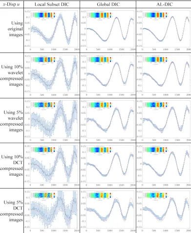
algorithms and the original as well as compressed images. The subset/mesh size is20×20. The strains for the Local Subset DIC are not shown because they are very noisy. . . 41 4.5 The displacement fields obtained from Local Subset DIC, Global

DIC, and ALDIC using original, wavelet, and DCT compressed im-ages of the heterogeneous fracture specimen. . . 43 4.6 The strain fields obtained from Global DIC and ALDIC using

orig-inal, wavelet, and DCT compressed images of the heterogeneous fracture specimen. . . 44 5.1 Comparison of adaptive Kuhn triangulation mesh and adaptive Quadtree

mesh. . . 55 5.2 All the 2D Kuhn triangles belong to one similarity class with different

orientations. . . 57 5.3 All kinds of elements in the Quadtree mesh, where nodes 1-4 are

(11)

5.6 Example of recursive refinement of 2D Quadtree mesh. . . 77

5.7 Comparison of solved Sample 14 L5 deformation field using adaptive regularized Global DIC with Kuhn triangulation and Quadtree mesh. 80 5.8 Comparison of solved Sample 14 L5 deformation field using adaptive ALDIC with Kuhn triangulation and Quadtree mesh. . . 81

5.9 Plot of a posteriori error estimates of SEM 2D-DIC synthetic images of Sample 14 L5 based on ADMM Subproblem 1 and Subproblem 2. 82 5.10 Comparison of a posteriori error estimate based on ADMM subprob-lem 1 local update and subprobsubprob-lem 2 global update. . . 82

5.11 (a) Collective cells under microscope. (b) DIC image with speckle pattern to measure collective cell migration. (Images courtesy of Jacob Notbohm.) . . . 82

5.12 Adaptive ALDIC solved collective cell migration using Kuhn adap-tive triangulation mesh. . . 84

5.13 Adaptive ALDIC solved collective cell migration using Quadtree adaptive mesh. . . 85

5.14 Comparison between solved collective cell migration using uniform Local Subset DIC, adaptive Kuhn triangulation ALDIC, and adaptive Quadtree mesh ALDIC. . . 86

5.15 Plot of a posteriori error estimates of cell migration based on ADMM Subproblem 1 and Subproblem 2. . . 87

5.16 Comparison of adaptive Local Subset DIC method, adaptive regular-ized Global DIC method and adaptive ALDIC method. . . 90

A.1 Matrix Din (a)4×4and (b)10×10FEM Q4 meshes where both element lengthh= 1. . . 94

C.1 Kuhn 3D simplex. (a) A 3D cube can be subdivided by three planar cuts in 6 similar Kuhn triangulation simplices. (b) Binary bisection tree of a 3D Kuhn triangulation simplex. . . 98

C.2 Adaptive 3D Octree mesh refinement. . . 99

C.3 3D Octree element template. . . 99

(12)

LIST OF TABLES

Number Page

3.1 List of symbols used in the demonstration section . . . 22 3.2 Comparison of the RMS errors in displacement and strain for the

SEM 2D-DIC synthetic images of Sample 14: L1, L3, and L5 . . . . 25 3.3 DIC displacement and strain RMS errors of Sample 14 L1 with

different window sizes . . . 26 3.4 List of symbols used in the analysis of computational cost . . . 31 3.5 The computation cost of the Local Subset DIC IC-GN iteration . . . 31 3.6 The computation cost of the Global DIC FEM iteration . . . 31 3.7 The computation cost of the ALDIC ADMM iteration . . . 32 3.8 Computation time using three DIC algorithms . . . 32 4.1 Mean and standard deviation of image compression induced greyscale

errors . . . 36 4.2 Absolute RMS errors of Sample 14 L1 data using three DIC

algo-rithms applied to the original images and the compressed images with different subset/mesh . . . 45 4.3 Relative RMS errors of Sample 14 L1 data using three DIC

algo-rithms applied to the original images and the compressed images with different subset/mesh . . . 46 4.4 Relative RMS errors of fracture experiment using three DIC

algo-rithms applied to the compressed images compared with results using the original images . . . 46 4.5 Computation time of the numerical demonstrations . . . 47 5.1 Comparison of the RMS errors in different DIC algorithms solved

displacement and strain for the SEM 2D-DIC synthetic images of Sample 14 L5 . . . 79 5.2 Computation time of adaptive regularized Global DIC using Quadtree

mesh to solve SEM-2D synthetic images of Sample 14 L5 . . . 83 5.3 Computation time of adaptive ALDIC using Quadtree mesh to solve

SEM-2D synthetic images of Sample 14 L5 . . . 87 5.4 Computation time of adaptive ALDIC using Kuhn triangulation mesh

to solve SEM-2D synthetic images of Sample 14 L5 . . . 87 5.5 Computation time of adaptive regularized Global DIC using Quadtree

(13)

5.6 Computation time of adaptive ALDIC using Quadtree mesh to solve collective cell migration . . . 88 5.7 Computation time of adaptive ALDIC using adaptive Kuhn

(14)

C h a p t e r 1

INTRODUCTION

Digital image correlation (DIC) is a popular optical experimental technique for measuring deformation and strain in solids. In this method, we decorate the surface of the sample with a speckle pattern. We then take a sequence of grayscale digital images of a test specimen during the deformation. Finally, by comparing images in the sequence, we determine the displacement and strain fields of the specimen using image tracking algorithms [1, 2, 3, 4].

DIC has several advantages compared with other strain measurement methods. First, unlike electrical resistance strain gauges that need to be glued on the sample surface, taking digital images does not require contact with the specimen. This is especially advantageous for soft materials where contact may affect strain fields. Second, each electrical resistance strain gauge only measures the strain status of one point but DIC can easily provide full field displacement and strain values. Compared with other non contact and full field optical strain measurement methods such as holographic methods, speckle methods, and interferometric methods [5, 6, 7, 8], DIC experiments do not require a very sophisticated experimental environment.

DIC has been applied to study the behavior of diverse solids systems such as bi-ological material [9, 10, 11], metal alloys [12], shape memory alloys [13], porous metals [14], polymers [15], and polymer foams [16]. It has provided insight into the very nonlinear behavior of solids like slip bands [13, 17] and crack tips [18]. This method can also be combined with other diagnostic tools to enable investi-gation of complex phenomena with very heterogenous and complex strain fields at various length scales from nanometers to kilometers. For example, DIC has been used to measure nonuniform phase transformation by combining scanning electron microscopy (SEM) and electron backscatter diffraction (EBSD) [19]. It has also been used with atomic force microscopy (AFM) to measure in-plane displacement at the nanometer scale [20]. At the other extreme, DIC has been used in earthquake and glacier monitoring [21, 22, 23, 24] at the scale of tens of kilometers.

(15)

[25, 26, 27, 28, 29]. In Local Subset DIC, as its name implies, we first break up both reference image and deformed image into many subsets and then find the deformation of each subset independently. Since the subsets are limited in size, the deformation of each subset can be solved very fast; moreover the subsets can be analyzed in parallel. Therefore, Local Subset DIC can be very fast. However, since the deformation of each subset is obtained independently, the overall deformation may not be compatible and the strain field can be extremely noisy. In Global DIC, we represent the global deformation using a basis set (often based on a finite element discretization), and then analyze the global image to obtain the coefficients relative to this basis set. However, this is expensive.

These considerations have led to a number of attempts to improve these methods. A number of filtering and smoothing schemes have been proposed to address the noisiness of the Local Subset DIC methods [30, 31, 32]. Broadly, filtering of both the images and the displacements not only reduces the noise but also can improve the accuracy because it incorporates information from surrounding regions. While this can be effective, the critical choice of filter is unrelated to the underlying mathematical structure and may be experiment dependent. Similarly, a number of sophisticated numerical methods have been introduced to address the computational cost of global methods. These have followed two key ideas, or a combination of the two. The first is to use either gradient [33, 34] or elastic [35, 36, 37] regularization. The second is to use domain decomposition where the domain is broken up into a number of domains, the correlation is performed compatibly in each sub-domain and the compatibility between the sub-sub-domains is enforced using either Lagrange multipliers [36, 38] or the finite element tearing and interconnecting (FETI) procedure [35, 37]. These can then be used in parallel implementation (see [39] for a review). These significantly speed up the convergence and reduce computational time. However, these require sophistication in their implementation and must be adopted to the problem at hand.

(16)

and its gradient equal the locally correlated values. We implement the constraint using the augmented Lagrangian method.

The augmented Lagrangian method, also known as the method of multipliers, has been used to solve constrained minimization problems in diverse fields [40, 41]. It adds to the objective functional a term that is linear in the constraint as in the method of Lagrange multipliers and a term that is quadratic in the constraint as in the penalty method. The addition of the quadratic term makes the numerical implementation easier than the method of Lagrange multipliers. However, unlike the penalty method, one does not need to take the limit of infinitely large penalty coefficients. For this reason, the augmented Lagrangian method has found widespread acceptance in both image precessing [42] and in mechanics [43, 44].

We implement the augmented Lagrangian using the alternating direction method of multipliers (ADMM) that is a form of operator splitting [45]. In this method, we successively perform the local correlation, optimize the auxiliary displacement, update the multiplier and iterate. The convergence and other numerical issues of ADMM have been carefully studied [46], and this method is widely used in image processing [45, 47, 48] and in mechanics [49]. The second problem, the optimization over the auxiliary displacement, is global. However, it leads to a universal, sparse, well-conditioned operator (sum of the Laplacian and identity). This can be treated very efficiently using established methods.

We compare the performance (accuracy and efficiency) of the new ALDIC algorithm with that of Local Subset DIC method and Global DIC method using both synthetic data (where the exact displacement is known) and experimental data. We show that ALDIC provides the most accurate displacement and strain. It is only a few times more computationally expensive compared to Local Subset DIC and significantly cheaper than Global DIC.

ALDIC also provides two additional advantages: it allows combining DIC with image compression, and it allows a multi-resolution approach.

(17)

is possible to obtain accurate displacement and strain fields with only 5% of the original image size. Among all three DIC methods (Local Subset DIC method, Global DIC method, and our proposed ALDIC method), Local Subset DIC leads to the largest errors and ALDIC to the smallest errors when compressed images are used. We also found that wavelet-based image compression introduces less error compared to DCT image compression techniques [50].

To further save the computation cost, especially in the study of complex hetero-geneous strain fields at various length scales, we apply h-adaptive finite element mesh with our proposed ALDIC method, which can be solved quickly. Compared to the current Global DIC method, this new adaptive ALDIC algorithm significantly decreases computation time with little loss (and some gain) in accuracy.

In this thesis, we review two current DIC algorithms, Local Subset DIC method and Global DIC method, in Chapter2. Next, we propose and describe a new image comparison algorithm: augmented Lagrangian DIC (ALDIC) in Chapter 3. We verify and evaluate the accuracy of the proposed ALDIC method using a series of case studies using synthetic data and experimental data in Section 3.5. These examples demonstrate the superior accuracy of the proposed ALDIC algorithm. We analyze the computation cost of the proposed method in Section 3.6. We show that the computational effort of the ALDIC is at worst a factor of two to four more expensive compared to Local Subset DIC method, and less expensive than the Global DIC method.

Chapter4introduces combining digital image correlation with image compression techniques. Specifically, Section 4.2 introduces two popular image compression techniques based on discrete cosine transform (DCT) and wavelet transform which we use in this thesis. We analyze the combination of the image compression techniques with three types of DIC algorithms in Section4.3. Section4.4provides various case studies with synthetic and experimental images. It shows that ALDIC combines naturally with wavelet transform based image compression.

(18)

(19)

C h a p t e r 2

REVIEW CURRENT DIC METHODS

In this chapter, we review DIC problem formulation and two popular categories of DIC algorithms which are Local Subset DIC method and Global DIC method. Local Subset DIC decomposes the domain into many local subsets, ignores the dependency between neighboring subsets, and can be solved fast and in parallel. In Global DIC method, the whole domain with all the subsets’ unknowns are solved together where the kinematic connection between neighboring subsets are automatically considered but it’s more expensive to solve and easily gets stuck into local minima.

2.1 Digital image correlation problem formulation

Consider a domainΩ⊂Rnundergoing a deformationy: Ω→Rn,(n = 2,3). As seen in Figure2.1, letXdenotes the reference or undeformed position of a particle inΩ andy(X)denotes the image or current position of the particle. Suppose we have a speckle pattern with grayscale valuef(X)in the reference domain, and the corresponding grayscale valueg(y)in the current configuration. If the deformation convects the grayscale, then we have

f(X) = g(y(X)). (2.1)

The problem of digital image correlation is the inverse problem of finding the deformation y(X)that satisfies (2.1) given grayscale images f(X)and g(y). We pose it as one of optimization, or one of finding the deformation map that minimizes

f(X) _f₍_X₎

X

X g(y(X)) g(y(X))

1 2

(20)

the squared difference:

C = Z

Ω

|f(X)−g(y(X))|2dX→_{minimize over}y: Ω→_Rn_.

(2.2)

A few comments are in order. First, the images are pixelated withf, gtaking discrete values. So we can either replace the integrals above with a sum, or interpolate the images (we use bi-cubic interpolation whenever we need sub-pixel values). Second, due to illumination artifacts and gain errors in real experiments, it is useful to normalize the images. This normalization depends on the knowledge of illumination and other experimental details. A simple example is to normalize both images to have the same mean and standard deviation:

f(X)7→ f(X)−f¯

σf

, g(y)7→ g(y)−g¯

σg

, (2.3)

wheref ,¯g¯are the mean values off, g, andσf, σgare their standard deviations [51].

Henceforth, we assume that we are always working with normalized images. Third, in light of the normalization, note that minimizing C is equivalent to maximizing the cross correlation _Z

Ω

f(X)g(y(X))dX. _(2.4)

Finally, in practice, there are different ways in which the correlation can be per-formed. One can take a series of images as the deformation proceeds and do the correlation between consecutive images, or one correlate the first and final image, or one can do something intermediate. The incremental correlation between suc-cessive image can lead to easier convergence and smaller individual errors due to small displacement, but can lead to the accumulation of systemic errors and add to the cost. These issues are common to all three algorithms that we discuss presently.

2.2 Local Subset DIC method

(21)

translation or piecewise affine.

y(X) = X+u(X) =X+X

i

(ui)χi(X) (Piecewise constant translation),

(2.5)

y(X) = X+u(X) =X+X

i

(ui+Fi(X−Xi0))χi(X) (Piecewise affine),

(2.6)

whereui is the translation vector of the center of the local subset Ωi, Fi is affine

deformation gradient tensor,Xi0is the coordinates of the center of each local subset,

χi is the characteristic or index function

χi =

(

1 X∈Ωi,

0 X∈/ Ωi.

(2.7)

Using piecewise translation ansatz (2.5), the optimization problem (2.2) decomposes into a number of decoupled problems of optimizating over four (n= 2) or six (n = 6) scalar variables:

Ci =

Z

Ωi

|f(X)−g(X+ui)|2dX →minimize overui. (2.8)

Using piecewise affine deformation ansatz2.6, the optimization problem (2.2) de-composes into a number of decoupled problems of optimizing over six (n = 2) or twelve (n= 3) scalar variables:

Ci =

Z

Ωi

|f(X)−g(X+ui+ (Fi(X−Xi0)))|2dX→minimize overFi,ui.

(2.9)

Problem2.8can be solved very fast using fast Fourier transform method [10]. As for problem2.9, there are a number of methods that have been used to solve this problem including the Inverse Compositional Gauss-Newton(IC-GN) [25, 26, 52] and Inverse Compositional Levenberg-Marquardt(IC-LM) scheme [52]. In this thesis, we use IC-GN and this is described in detail in2.3and summarized in Algorithm1.

2.3 Inverse Compositional Gauss-Newton (IC-GN) scheme

Here we summarize the Inverse Compositional Gauss-Newton (IC-GN) scheme to solve Local Subset DIC optimization problem.

(22)

Algorithm 1:Local Subset DIC

Input: Reference imagef, deformed imageg

Output: Displacementui, affine deformation gradient tensorFiof each local subset

Step 1: Initialization using FFT integer pixel search method; Step 2: Precompute image gradients∇g;

Step 3: _{For each local subset, compute}aip, biqr, cjkqr using (2.14), (2.15), (2.16); whilekdik,kejkk> εdo

Step 4: Warp deformed imagegwith current deformationFi,ui ; Step 5: _Computedi, ejk using (2.17), (2.18);

Step 6: Computev,Husing (2.13) ; Step 7: Updateφusing (2.11) end

φk(yk₍_X_{)) =} _X

. We define the incrementψkthroughyk+1 = ψk◦yk as shown in Figure2.2. We make a change of configuration and rewrite as

Ci =

Z

Ωk i

|f(φk(z))−g(ψ(z))|2dz, (2.10)

wherezis the current iterate of deformation mapyk. We obtainψkas the minimizer of this functional and the updated deformation map as

φk+1 =φk◦(ψk)−1. (2.11)

To minimize (2.10), we assume ψk ≈ z +v+H(z−z0) for small v and H. Therefore,

Ci =

Z

Ωk i

|f(φk(z))−g(z)− ∇g(z)·(v+H(z−z0))|2dz. (2.12)

Minimizing overvandH, we obtain

alp blqr

bmnp cmnqr

!

vp

Hqr

!

= dl

emn

!

(23)

Figure 2.2: The change of variables involved in the IC-GN update.

where

alp = 2

Z

Ωk i

g,lg,pdz, (2.14)

blqr =

Z

Ωk i

g,lg,q(zr−z0r)dz, (2.15)

cmnqr = 2

Z

Ωk i

g,m(zn−z0n)g,q(zr−z0r)dz, (2.16)

dl =

Z

Ωk i

(f −g)g,ldz, (2.17)

emn =

Z

Ωk i

(f −g)g,m(zn−z0n)dz, (2.18)

andg,l = _∂∂g

zl etc. We solve (2.13) forv,Hto obtainψ k

. We then obtain the new (inverse) deformationφk+1using (2.11). In practice, we don’t need to computeΩki

domain at each iteration, instead we directly compute all the integrations (or discrete summations) over the final deformed configuration, which also gives us good results and saves lots of computation time.

Since the problems are decoupled, i.e., can be solved independently for eachi, local subset DIC is extremely fast and easily paralellized. Further, in practice, the subsets can overlap. However, since each problem is solved independently, the results can be noisy, susceptible to local imaging problems, and lead to discontinuous strain fields.

2.4 Global DIC method

(24)

Local DIC Global DIC

Figure 2.3: Comparison between Local Subset DIC and Global DIC.

(see Figure2.3right):

y(X) =X+u(X) =X+X

p

upψp(X), (2.19)

whereψp(X)are the chosen global basis functions andupare the unknown degrees

of freedom. Thus, the problem (2.2) becomes

Cg =

Z

Ω

f(X)−g(X+X

p

upψp(X))

2

dX →minimize over{up}. (2.20)

We can solve this problem iteratively by settinguk+1 =uk+δuand using the first

order approximation

g(y(X)) =g(X+uk(X) +δu)≈g(X+uk(X)) +∇g·δu(X) (2.21)

so that

Cg ≈

Z

Ω

f(X)−g(X+uk(X))−

X

p

δupψp(X)

!

· ∇g(X) 2

dX. (2.22)

This leads to the linear equation inδu

Mpqδuq =bp, (2.23)

where

Mpq =

Z

Ω

ψT_p(X) (∇g) (∇g)T ψ_q(X)dX, (2.24)

bp =

Z

Ω

(25)

Alternately, if the displacements are small, we can treat (2.23) as a linear problem withδuas the incremental displacement.

Note that the size of the linear problem (2.23) is equal to the number of basis functions or the size of the finite element discretization. This can be large if we seek fine resolution. Thus, Global DIC is expensive and difficult solve in parallel. However, it leads to compatible solutions. And there are methods to reduce the computational expense as discussed in the introduction. In practice, it is common to replace∇gwith∇f or to use IC-GN which deals with the inverse map. This has the advantage that the matrixMpq is independent of iteration thereby reducing the

effort.

We remark that the procedure described in (2.23-2.25) may result in noisy displace-ment fields because of the conditioning of the matrixM. So it is common practice to add a weighted higher order penalty (regularizer) to the objective function. This needs experience and expertise. Further, this requires boundary conditions whose choice can lead to errors.

Finally, note that the Global DIC is not limited to smooth fields. It can be used to study discontinuous fields like cracks and shear bands by using enriched basis [53, 54]. In this paper, we use a Q4 finite element mesh in Global DIC, and this is summarized in Algorithm2.

2.5 Global DIC with regularization

In Global DIC method, besides the guarantee of displacement continuity, we can also assume there is certain smoothness in the displacement field. Thus, the regularized Global DIC is the method which modifies Global DIC to prefer displacement field with some smoothness by adding higher order regularizer termαhBu(X),u(X)i onto the original correlation function in (2.20). 1

The new correlation functionCg−RGchanges to be

Cg−RG =

Z

Ω

[f(X)−g(X+u(X))]2+αhBu(X),u(X)i. (2.26)

NotationhBu(X),u(X)imeans the inner product betweenBu(X)andu(X), which explicitly is thatBu(X)multipliesu(X)and then integrate over the whole domain. There are various choices of operator Bto add this smoothness penalty term. For

1

(26)

Algorithm 2:Q4 Global DIC

Input: Reference imagef, deformed imageg Output: Displacementu

Step 1: _{Initialization using FFT integer pixel search method;} Step 2: Precompute image gradients∇g;

foreachpixel in each finite elementdo

Step 3: _{Compute isoparametric element local coordinates ;} Step 4: Compute isoparametric elementψmatrix ;

Step 5: Compute isoparametric element JacobianJmatrix; Step 6: _{Compute spatial gradient of}ψ_matrix: Dψ_;

Step 7: Assemble onto stiffness matrixM=M+ [ψT∇g][ψT∇g]T using (2.24);

Step 8: (Optional) Add regularizer term onto stiffness matrix, e.g.

α[Dψ]T_[_D_ψ_]

end

whilekδuk> εdo

Step 9: Warp deformed imagegwith current displacementun; Step 10: _{Assemble vector}b_{using (2.25);}

Step 11: Add regularizer term onto vectorbif Step 8has been done ; Step 12: Solveδuby (2.23) ;

Step 13: _{Update displacement}uk+1 =uk+δu; end

example, whenBequals the identity matrixI, this approach is also called Tikhonov regularization [55]. WhenB equals the Laplace operator, this method is gradient regularization [33, 34]. Ref [34]§9 uses elastic potential energy as a Global DIC regularizer, where uses a positive definite bilinear operator, to introduce a global constraint of smoothness as:

B[u,v] = Z

Ω

λdiv(u)div(v) + 2µ 2 X

i,j=1

eij(u)eij(v). (2.27)

Hereeij(u) = 1/2(∂ui/∂xj+∂uj/∂xi)is the small strain tensor, andλ >0, µ >0

are so-called Lamé constants of the materials’ elastic properties. All the above regu-larization choices are good for small deformations. As for large deformations, fluid regularization [56], hyper-elastic regularization [57], and curvature regularization [58] have also been proposed recently.

(27)

strict Sobolev space, but also that it helps optimization converge faster and avoid local minima in the numerical respect.

Theoretically, all these regularized Global DIC could more or less help improve displacements result’s smoothness. However, if the displacements field is heteroge-neous and not quite uniform, the displacements’ accuracy is quite sensitive to the choice ofBoperator and the regularization term weightα. Too largeαwill smooth out the heterogeneity of displacement fields, while too smallαdoesn’t help improve the noise obviously. Choosing operator B and parameter α is still mostly based on the researcher’s experience and preference. What’s more, as for displacement field with high heterogenuity, varying regularization term coefficientsα is needed instead of just one fixed value [59].

Adding regularizer terms can help Global DIC converges faster, however, it is still an expensive method. Note that the size of the linear problem (2.23) is equal to the number of basis functions or the size of the finite element discretization. This can be large if we seek fine resolution. And since the highly oscillating characteristics of the speckle patterns, standard Gaussian quadrature usually fails in the computation of stiffness matrix{Mpq}and external force vector{bp}. Instead, these numerical integral in are approximated by direct pixelwise summations, which make the Global DIC method expensive. And since all the unknowns in finite element discretization are solved together, the procedure described in Eqs(2.23-2.25) may still need a large number of iterations until converged.

2.6 Conclusion

(28)

C h a p t e r 3

AUGMENTED LAGRANGIAN DIC METHOD

[1] J Yang and K Bhattacharya. “Augmented Lagrangian digital image correla-tion”. In:Experimental Mechanics. Under review(2018).

We introduce a new image comparison algorithm, augmented Lagrangian DIC (ALDIC) in this chapter, which seeks to combine the advantages of both the Local Subset DIC (speed and parallel implementation) and the Global DIC (displacement compatibility and strain smoothness).

3.1 ALDIC formulation

Recall the ansatz (2.5) we made in Local Subset DIC method. In this ansatz, the local displacement ui and local displacement gradient Fi in the subdomain Ωi are independent of each other, and independent for each i. Thus, there is no

guarantee of compatibility for the deformation. However, if the displacement field were compatible, then the displacements and the displacement gradients would not be independent, but instead satisfy a global constraint

{F}=D{u}, (3.1)

whereDis an appropriate discrete gradient operator (see AppendixAfor examples of first order finite differences). The Local Subset DIC ignores this constraint while the Global DIC enforces this constraint by kinematic construction.

The key idea of ALDIC is to treat this constraint (3.1) efficiently. We do so by leaving

Fi andui discrete as before, and introduce an auxiliary compatible displacement

fielduˆsuch that

Fi =∇uˆ(Xi0), ui = ˆu(Xi0). (3.2) In other words, we minimize (2.2) subject to the ansatz (2.5) and constraints (3.2). We do so using an augmented Langrangian method. Specifically, we consider the correlation functional

L0 = X

i

Z

Ωi

|f(X)−g(X+ui+ (Fi(X−Xi0)))| 2

+ β

2|(Dˆu)i−Fi| 2

+νi : ((Dˆu)i−Fi) +

µ

2|uˆi−ui| 2

+λi·((ˆu)i−ui)

dX,

(29)

where we use the matrix or Frobenius norm for matrices|A|2 =Pij|aij|

2

, vector norm for vectors|a|2 = Pia

2

i, and:for double dot product between two matrices

A :B=P

ijAijBij. Above,{νi}, {λi}are Lagrange multipliers that enforce the

constraints (3.2). Finally,β andµare two positive real scalars. Ifβ =µ= 0, then this functional gives the traditional Lagrange multiplier formulation if we change the sign of{νi},{λi}. On the other hand ifβandµwere very large withνi =λi =0,

then we have a penalty method. Choosing β and µ to be positive real scalers while retaining the Lagrange multipliers is referred to as the augmented Lagrangian method, and gives rise to well-conditioned numerical problems [40].

Given β and µ, we iteratively minimize L0 {Fi},{ui} and {uˆi}and update {νi}

and{λi}. Before we proceed, it is convenient to make the following modification

to the functional above. We setWi :=νi/β,vi :=λi/µand define

L =X

i

Z

Ωi

|f(X)−g(X+ui+ (Fi(X−Xi0)))|2

+β

2 |(Dˆu)i−Fi+Wi| 2

+µ

2|uˆi−ui+vi| 2

dX.

(3.4)

Notice that minimizingL0over{Fi},{ui}and{uˆi}is the same as minimizing over

Lsince they differ by quadratic terms independent of{Fi},{ui}and{uˆi}.

The functional L is not local because the discrete derivative (Dˆu)i depends on

the value of ˆui in neighboring subsets. Thus, we still obtain a global problem as

in the Global DIC method. However, there are two reasons why this problem is computationally easier. First, the only non-local term is quadratic with a constant scalar coefficient. Therefore it can be minimized very easily. Second, we can solve this problem using an alternating direction method of multipliers (ADMM) that allows us to break it up into simpler problems.

3.2 Alternating direction method of multipliers (ADMM)

We use alternating direction method of multipliers (ADMM) where local subprob-lems are coordinated to find a solution to a large global problem [46] to iteratively solve the problem.

Given{Fki},{uki},{uˆki},{Wki},{vik}, we find the(k+ 1)th update as follows:

• Subproblem 1: local update. While holding{uˆki},{Wik},{vki}fixed,

mini-mizeLover{Fi},{ui},to obtain{Fki+1},{u k+1

i }:

{Fk_i+1},{uk_i+1}= arg min

{Fi},{ui}

L {Fi},{ui},{uˆki},{W k i},{v

k i}

(30)

Since{uˆki}and hence{(Duˆ)ki}are known, this problem breaks into a series

of local problems that can be solved independently for eachi:

Fk_i+1,uk_i+1 = arg min

Fi,ui

Li = arg min

Fi,ui

Z

Ωi

|f(X)−g(X+ui+ (Fi(X−Xi0)))| 2

+β 2

(Dˆu)k_i −F_i+W_ik 2 + µ 2

uˆk_i −u_i+v_ik

2

dX.

(3.6)

This is similar to Local Subset DIC and can be solved by any of the methods described in Section2.2.

• Subproblem 2: global update. While holding {Fki+1},{u k+1

i },{Wki},{vki}

fixed, we minimizeLover{uˆi}to obtain{uˆki+1}:

{uˆk_i+1}= arg min

{ˆui}

L {Fk_i+1},{uk_i+1},{uˆi},{Wki},{vki}

= arg min

{ˆui}

X i Z Ωi β 2

(Dˆu)i −Fki+1+W k i 2 +µ 2

uˆi −uki+1+v k i

2

dX.

(3.7)

Note that this is a global problem, but is independent of the images f, g. Indeed, it leads to the linear problem

βDTD+µIuˆk+1 = βDTa+µb, (3.8)

wherea={Fki+1−Wki}andb={u k+1

i −vki}. The solution is given by

ˆ

uk+1 = βDTD+µI−1 βDTa+µb. (3.9)

Since β and µ are fixed, the matrix βDTD+µI

−1

can be precomputed and stored, and therefore this step becomes a simple matrix-vector multipli-cation. Further, the matrixDhas a structure, and therefore this matrix-vector multiplication can be carried out very efficiently.

• Subproblem 3: Lagrange multiplier update. We finally update{Wi},{vi}as follows:

Wk_i+1 =W_ik+ (Dˆu)k_i+1−Fk_i+1, (3.10)

vk+1 =vk+ uˆk+1−uk+1. (3.11)

(31)

The overall algorithm is summarized in Algorithm3.

Algorithm 3:_ALDIC

Input: Reference imagef, deformed imageg

Output: _Displacementui, deformation gradient tensorFiof each local subset, global displacementuˆ

Step 1: Initialization using FFT integer pixel search method; Step 2: _{Precompute finite difference operator}D_;

Step 3: Choose initial parametersβ,µ. Set dual variablesW,vto be zero; whileuk+1−uk

> εand

ˆuk+1−ˆuk

> εdo

Step 4: Solve subproblem 1 (3.6) as in Algorithm1foruk+1,Fk+1,; Step 5: Solve subproblem 2 (3.9) foruˆk+1 ;

Step 6: _{Update dual variables}W,v_{by (3.10), (3.11);}

end

3.3 Extensions of ALDIC algorithm

A simplification of Subproblem 1

While holding {uˆki},{Wki},{vik} fixed, minimize L over {Fi},{ui}, to obtain {Fk_i+1},{u_ik+1}_{. Since} {uˆk

i}and hence{(Duˆ)ki} are known, this problem breaks

into a series of local problems that can be solved independently for eachias in Local Subset DIC, which can be solved in parallel and converges fast near the 6-parameter optimal solution using IC-GN scheme analogously with (2.13), wherealp,dl,cmnqr

andemnare replaced with

a0_lp = 2 Z

Ωk i

(g,lg,p+

µ

2δlp)dz, (3.12)

d0_l = Z

Ωk i

((f −g)g,l+

µ

2(ul−v

k l −uˆ

k

l))dz, (3.13)

c0_mnqr = 2 Z

Ωk i

g,m(zn−z0n)g,q(zr−z0r) +

β

2δmqδnr

dz, _(3.14)

e0_mn = = Z

Ωk i

(f−g)g,m(zn−z0n) +β(Fmn−(Duˆ)kmn−Wmnk )

.(3.15)

(32)

ALDIC Subproblem 1 as follows: in the (k+ 1)th iteration step, we update Fk+1 to be exactly equal to Dˆuk and only solve for uk+1. We still use the same IC-GN iteration method as introduced previously in Section2.2 Local Subset DIC, where

uk+1

are solved by

uk_p+1

i =

a0_lp −1

i {d 0

l}i. (3.16)

Extension ALDIC to arbitrary mesh

In the second subproblem (3.7), in the alternating direction, we fixF, uand try to updateuˆby:

ˆ

uk+1 = arg min

ˆ u

β

2

Dˆu−Fk+1+Wk 2

F +

µ

2

ˆu−uk+1+vk 2

L2 (3.17)

Using regular uniform mesh, analytical solution foruˆ can be computed fast using sparse matrix computation.

ˆ

uk+1 = βDTD+µI−1

βDTa+µb

. _(3.18)

Sinceβ, µare both positive scalars, it’s easy to prove βDTD+µIis symmetric positive definite, therefore it always has inverse.

ALDIC algorithm ADMM scheme works not only for uniform square mesh, but also for arbitrary general mesh. If we are using non-uniform mesh, Subproblem 1 can be easily extended to solve local update problems around each node of the non-uniform mesh. Subproblem 2 can still be solved fast through

(β∆−µI)ˆu=β∇ ·(Fk+1−Wk)−µ(uk+1−vk+1). (3.19)

(3.19) will be discussed in details in Section5.3where we apply adaptive mesh onto ALDIC.

Using non-uniform mesh, the Subproblem 3 Lagrange multipliers update step will also be changed to

(

Wk_i+1 =Wk_i + ((∇uˆ)k_i+1−Fk_i+1)

v_ik+1 =vk_i + (ˆu_ik+1−uk_i+1) (Lagrangian multipliers update). (3.20)

3.4 Convergence and optimal conditions of ADMM

Convergence of ADMM

(33)

• Assumption 1. The functional Ci in (2.9) or the first term of L can be approximated by a closed, proper, and convex functional near the optimal solution.

• Assumption 2. The LagrangianL0 withβ = µ= 0 has a saddle point; i.e., there exist({F∗i},{u

∗ i},{uˆ

∗ i},{ν

∗ i},{λ

∗

i}), for which

L0({F∗i},{u ∗ i},{ˆu

∗

i},{νi},{λi})≤ L0({F∗i},{u ∗ i},{ˆu

∗ i},{ν

∗ i},{λ

∗ i})

≤ L0({Fi},{ui},{ˆui},{ν∗i},{λ ∗ i})

for all({Fi},{ui},{uˆi},{νi},{λi}).

Then, we have the following convergence results:

• Primal residual convergence. Dˆuk−Fk → 0 and uˆk−uk → 0 as

k → ∞_{, i.e., the constraints are satisfied asymptotically;}

• Dual residual convergence. uˆk+1−uˆk → 0 as k → ∞, i.e., the dual feasibility is satisfied asymptotically, see (3.26).

• Objective convergence. Lk → L∗ask → ∞, i.e., the Lagrangian approaches its optimal value;

• Dual variable convergence. Wk → W∗,vk → v∗ as k → ∞, where (W∗,v∗)is dual optimal point.

Note that the local functionalCi can be highly oscillatory and is thus not convex. However, if the initial guess for the local variables({Fi},{ui})is in the convergence basin of Local Subset DIC, then the first assumption is true. If this assumption is false, then subproblem 1 (3.5) above diverges; this provides a check that this assumption holds.

Optimality conditions of ADMM

Set the first term in (3.4) to be

Φ(F,u) = X

i

Z

Ωi

|f(X)−g(X+ui+ (Fi(X−Xi0)))| 2

dX. (3.21)

The necessary and sufficient optimality conditions for the ALDIC ADMM formu-lation are primal feasibility,

"

Dˆu∗−F∗ ˆ

u∗−u∗

#

= "

0 0

#

(34)

and dual feasibility,

"_∂_Φ(_F∗_,_u∗₎

∂F

∂Φ(F∗_,_u∗₎

∂u #

− "

βW∗

µv∗

# = " 0 0 # . _(3.23)

SinceFk+1,uk+1 minimizeL(F,u,ˆuk,Wk,vk)in the ADMM Subproblem 1, we have that " 0 0 # =

"_∂_Φ(_Fk+1_,_uk+1₎ ∂F

∂Φ(Fk+1_,_uk+1₎ ∂u

# −

"

βWk

µvk

# −

"

β Dˆuk−Fk+1

µ uˆk−uk+1

#

=

"_∂_Φ(_Fk+1_,_uk+1₎ ∂F

∂Φ(Fk+1,uk+1)

∂u #

− "

βWk

µvk

# −

"

β Dˆuk+1₋_Fk+1

µ uˆk+1−uk+1

# −

"

β Dˆuk₋_Dˆ_uk+1

µ uˆk−uˆk+1

#

=

"_∂_Φ(_Fk+1_,_uk+1₎ ∂F

∂Φ(Fk+1,uk+1)

∂u #

− "

βWk+1

µvk+1 #

− "

µ uˆk₋_u_ˆk+1 #

.

(3.24)

Or equivalently,

"_∂_Φ(_Fk+1_,_uk+1₎ ∂F

∂Φ(Fk+1_,_uk+1₎ ∂u

# −

"

βWk+1

µvk+1 #

= "

µ ˆuk₋_ˆ_uk+1 #

. (3.25)

This means that the quantity

sk+1 = "

β Dˆuk−Dˆuk+1

µ ˆuk₋_u_ˆk+1 #

(3.26)

can be viewed as a residual for the dual feasibility condition (3.23). We will refer to

sk+1

as the dual residual at ADMM (k+ 1)th iteration, and to

rk+1 = "

Dˆuk+1₋_Fk+1

ˆ

uk+1₋_uk+1 #

(3.27)

as the primal residual at ADMM (k + 1)th iteration. And these two residuals converge to zeros as ADMM proceeds.

3.5 Demonstration

We now demonstrate the ALDIC method, and compare it to both Local Subset DIC and Global DIC methods. All algorithms are implemented in Matlab. We use the following parameters unless it is specified otherwise. We use bi-cubic interpolations for the grayscale value at subpixel positions. In the Local Subset DIC, we stop IC-GN iterations whenkdik,kejkk < 10−6. Usually the IC-GN reaches convergence

(35)

Table 3.1: List of symbols used in the demonstration section

Fk

Solved deformation gradient tensor in thek-th ADMM iteration Subproblem 1

uk

Solved displacement vector in thek-th ADMM iteration Subproblem 1

uk

Solved displacement vector in thek-th ADMM iteration Subproblem 2

Wk_,_vk

Dual variables in thek-th ADMM iteration

u_, x_{-direction displacement component}

v_, y_{-direction displacement component}

exx, eyy, exy The “xx”,”yy” and “xy” components of infinitesimal strain

with a bilinear form of the domain’s displacement field trying to approximate the exact nonuniform one. We stop the iteration when the average magnitude of the nodal displacement update is smaller than10−6pixels. In ALDIC, we startWandv from zero. We chooseµto beO(10−3)∼O(10−1)times diagonal terms ofa0ip. We

takeβ=O(10−1)∼O(100)·element size2·µto balance the relevant terms. We use the same stop criteria in subproblem 1 as Local Subset DIC (kd0ikL2 < 10

−6 ), and the whole ALDIC iteration stops whenuˆk+1−uˆk

_L

2 <10 −4

.

When studying synthetic images where the exact deformation is known, we use the root-mean-square (RMS) error,

RMS error:= v u u u t

X

#of nodes

|Numerical result−Exact value|2

#of nodes (3.28)

in both the displacement and strain. RMS error reflects globally how far the com-puted results are away from the exact values and is a measure of the standard variance of the computation error.

In Local Subset DIC, we report the deformation gradients/strains obtained directly by the Local Subset DIC correlation. In Global DIC, we compute nodal strains by extrapolating the strains from the finite element Gauss points. In ALDIC, the strain field is obtained directly from Duˆ. We summarize the symbols we used in the demonstration section in Table3.1.

Case study I: Synthetic images from the SEM 2D-DIC Challenge

We study synthetic images from the SEM 2D-DIC challenge, samples 1 & 14 [60]1. Sample 1 represents a series of pure translations while Sample 14 represents a sinusoidal deformation with changing frequency.

1

(36)

[image:36.612.109.505.67.303.2]

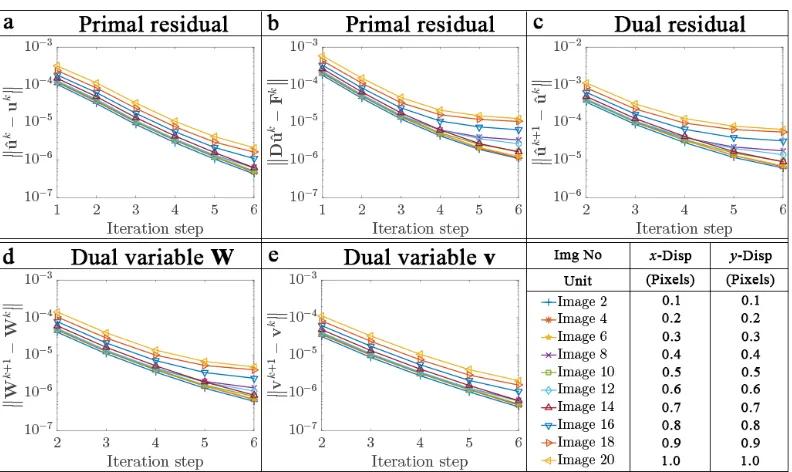
Figure 3.1: Convergence of the ALDIC method for the SEM 2D-DIC synthetic images, Sample 1 representing translation.

Translation: Sample 1

The deformations in Sample 1 are pure translations in both x and y directions with amplitudes ranging from 0 to 1 pixel in increments of 0.1 pixels. We set all the local window sizes to be 20×20 pixels, and set both the local neighboring windows distance and global element size to be 5×5 pixels. Figure 3.1 shows the convergence of the various quantities (without a stopping criterion). We see that ALDIC behaves well and converges within 6 steps. Figure3.2shows the RMS errors in displacements and strains, and compares with the corresponding errors in the Local Subset DIC and Global DIC methods. We observe that ALDIC has the smallest errors in all cases.

(37)

[image:37.612.108.505.414.633.2]

Figure 3.2: Comparison of RMS error in displacement (a) and strain (b) computed with the three methods for the synthetic images in the SEM 2D-DIC, Sample 1 or translation.

(38)

Table 3.2: Comparison of the RMS errors in displacement and strain for the SEM 2D-DIC synthetic images of Sample 14: L1, L3, and L5

Image local subset Regularized ALDIC

No DIC Global DIC

x displacement (pixels)

L1 0.0212 0.0080 0.0139

L3 0.0202 0.0162 0.0136

L5 0.0201 0.0234 0.0141

Strainexx

L1 3.18×10−3 3.15×10−4 9.83×10−4 L3 3.19×10−3 1.90×10−3 9.84×10−4 L5 3.20×10−3 3.10×10−3 1.00×10−3

Heterogeneous deformation: Sample 14

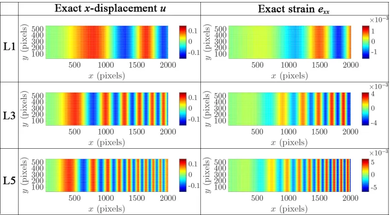
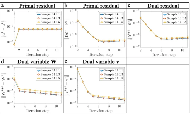
The deformations in Sample 14 are sinusoidal with varying frequency in the x direction as shown in Figure 3.3 for the three images — L1, L3, and L5 — that we use. It has zero displacement in the y direction. We set all the local window sizes to be30×30pixels, and set both the local neighboring windows distance and global element size to be 5×5pixels. As before, the ALDIC method converges in about six iterations (we have omitted the figure for brevity). Figures3.5and3.6 show the horizontal displacement u and the horizontal longitudinal strain exx for the three images and the three methods. These figures show that the ALDIC leads to smooth displacement fields and this is reflected in the strain. Table3.2shows the RMS errors for strain and displacement, and shows that the ALDIC method leads to smaller errors compared to the other two methods.

We also use the image L1 from this set to study the effect of the subset size in the ALDIC method. Table3.3shows the RMS errors in displacement and strain using three window sizes. Not surprisingly, the errors increase with decreasing window size.

Case study II: Experimental heterogeneous fracture deformation

(39)

[image:39.612.108.505.67.305.2]

Figure 3.4: Convergence check of ALDIC algorithm in Sample 14 L1, L3, and L5.

Table 3.3: DIC displacement and strain RMS errors of Sample 14 L1 with different window sizes

Subset Local Subset Regularized ALDIC

Size DIC Global DIC

x displacement (pixels)

30×30 0.0199 0.0079 0.0056

20×20 0.0323 0.0082 0.0067

10×10 0.0990 0.0088 0.0165

Strainexx

30×30 3.30×10−3 2.08×10−4 9.57×10−5 20×20 7.78×10−3 2.35×10−4 1.62×10−4 10×10 9.90×10−2 2.84×10−4 8.19×10−4

(40)

[image:40.612.109.505.164.579.2]

(41)

[image:41.612.109.506.166.578.2]

(42)

[image:42.612.179.437.71.358.2]

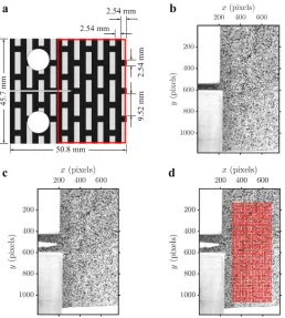
Figure 3.7: Heterogeneous specimen used for the third case study. (a) Front view of designed fracture specimen with brick architecture, where the box area will be captured using a CCD camera. (b) A speckle pattern is applied using white spray paint onto the surface of the specimen where the length scale of the digital image is 0.037mm/pixel. (c) One deformed image of the sample as the crack propogates under loading. (d) The local subsets/global finite element mesh used in all three DIC methods.

DIC, which in turn is less noisy than the Local Subset DIC. This is also reflected in the strain fields.

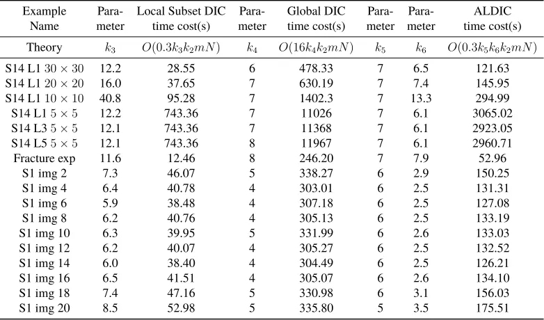
3.6 Computational cost

We compare the computational cost of the three DIC algorithms. The symbols used are listed in Table 3.4. We estimate the cost of each step in each algorithm, and these are listed in Tables3.5-3.7. We then use the dominant terms (assuming that

k1 << k2) to estimate the total cost, and these are also listed in the tables. We

(43)

[image:43.612.107.504.74.307.2]

Figure 3.8: Convergence of ALDIC method in heterogeneous fracture experiment.

[image:43.612.107.507.356.669.2]

(44)

Table 3.4: List of symbols used in the analysis of computational cost

N #_{of pixels in each local subset or each finite element}

m #of total local subsets or finite elements

d The dimension of images, e.g. d= 2for 2D pixel images

nL Length of parameter vectors of each local subset

nG Length of parameter vectors in finite element

k1 Computation cost to compute image grayscale derivatives

k2 Computation cost to interpolate grayscale value at sub-pixel position

k3 #of iterations in Local Subset DIC algorithm

k4 #of iterations in Global DIC algorithm IC-GN scheme

k5 #of iterations in ALDIC ADMM scheme

k6 #of inside iterations in ALDIC Subproblem 1 IC-GN scheme

C #of clusters used in Local Subset DIC and ALDIC Subproblem 1 for parallel computation

Table 3.5: The computation cost of the Local Subset DIC IC-GN iteration

Pre-computation _{Step 2} _{Step 3}

O(k1dmN) O(nL2mN)

Per IC-GN iteration _{Step 4} _{Step 5} _{Step 6} _{Step 7}

O(k2nLmN) O(nLmN) O(nL3m) O(nL3m)

Total O(k2k3nLmN/C)

Table 3.6: The computation cost of the Global DIC FEM iteration

Pre-computation Step 2 Step 3 Step 4 Step 5

O(k1dmN) O(dn3GmN) O(dnGmN) O(d2nGmN)

Step 6 Step 7 Step 8

O(d6nGmN) O(d4n2GmN) O(d

4

n2GmN)

Per FEM iteration Step 9 Steps 10-11 Step 12 Step 13

O(k2dnGmN)O(d2nGmN) O(dnGm) O(dnGm)

Total O(k2k4d2nGmN)

(45)

[image:45.612.111.502.221.451.2]

Table 3.7: The computation cost of the ALDIC ADMM iteration

Pre- _{Steps 2-3}

computation O(2d2_m₎

Per ALDIC Step 4 Step 5 Step 6 iteration O(k2k6nLmN) O(2d3m2) O(nLm)

Total O(k2k5k6nLmN/C)

Table 3.8: Computation time using three DIC algorithms

Example Para- Local Subset DIC Para- Global DIC Para- Para- ALDIC Name meter time cost(s) meter time cost(s) meter meter time cost(s)

Theory k3 O(0.3k3k2mN) k4 O(16k4k2mN) k5 k6 O(0.3k5k6k2mN)

S14 L130×30 12.2 28.55 6 478.33 7 6.5 121.63

S14 L120×20 16.0 37.65 7 630.19 7 7.4 145.95

S14 L110×10 40.8 95.28 7 1402.3 7 13.3 294.99

S14 L15×5 12.2 743.36 7 11026 7 6.1 3065.02

S14 L35×5 12.1 743.36 7 11368 7 6.1 2923.05

S14 L55×5 12.1 743.36 8 11967 7 6.1 2960.71

Fracture exp 11.6 12.46 8 246.20 7 7.9 52.96

S1 img 2 7.3 46.07 5 338.27 6 2.9 150.25

S1 img 4 6.4 40.78 4 303.01 6 2.5 131.31

S1 img 6 5.9 38.48 4 307.18 6 2.5 127.08

S1 img 8 6.2 40.76 4 305.13 6 2.5 133.19

S1 img 10 6.3 39.95 5 331.99 6 2.6 133.03

S1 img 12 6.2 40.07 4 305.27 6 2.5 132.52

S1 img 14 6.0 38.40 4 304.49 6 2.5 126.21

S1 img 16 6.5 41.51 4 305.07 6 2.6 134.10

S1 img 18 7.4 47.16 5 330.98 6 3.1 156.03

S1 img 20 8.5 52.98 5 335.80 5 3.5 175.51

3.7 Conclusion

In this chapter, we have presented a new method, the augmented Lagrangian digital image correlation (ALDIC), for image matching. It combines the advantages of the two established methods, the speed of Local Subset DIC and the kinematic compatibility of Global DIC. We show in Section 3.5 through a series of case-studies using synthetic images that ALDIC provides superior accuracy compared to the established methods. We show in Section3.6that the computational cost of ALDIC is only a few times that of Local Subset DIC and less than that of Global DIC.

(46)

Figure 3.10: Comparison of the deformation gradient (F11 component) obtained using the Local Subset DIC (a) and ALDIC (b) for Sample 14 L1.

correlation or sub-problem 1 has some global information through the augmented Lagrangian and auxiliary field — see equation (3.6). Second, the auxiliary field leads to less noisy deformation gradients as shown in Figure3.10. However, ALDIC is more expensive than Local Subset DIC because it requires the solution of a global problem (3.8) and it undergoes ADMM iterations. Still, this is not prohibitive: we see in Section3.6that it is only a few times that of Local Subset DIC.

Both ALDIC and Global DIC seek to impose compatibility. However, the point of departure is that ALDIC does not use a basis set to impose compatibility anywhere, but does so using an augmented Lagrangian. Therefore, the resulting operator (βDTD +µI) is the sum of the Laplacian and identity. This is universal, i.e., independent of the problem, displacement or image (though the matrix depends on the discretization). The nature of the operator and the universality allows us to either precompute the inverse (as we do here), or us a variety of established efficient methods (see for example [63]). In contrast, the operator M in (2.24) depends on the image, and moreover may be poorly conditioned depending on the image. Regularization can help with the conditioning and it is possible to address the computational cost. However, these require sophistication in their implementation and must be adopted to the problem at hand.

(47)

Local DIC Global DIC

AL-DIC Subproblem 2 solved globally AL-DIC Subproblem 1

solved locally

ADMM

(48)

C h a p t e r 4

COMBINING DIC WITH IMAGE COMPRESSION

TECHNIQUES

[1] J Yang and K Bhattacharya. “Combining image compression with digital image correlation”. In:Experimental Mechanics. Under review(2018).

4.1 Introduction

Digital imgage correlation(DIC) infers the deformation from changes in the images of speckle patterns. Therefore, it is necessary to have high resolution images to obtain accurate displacement and strain values. Further, for the convergence and efficacy of the image conversion algorithms, it is useful to keep the relative deformation small. So it is common to acquire a series of images of the deformation process. For all these reasons, DIC requires the acquisition, transmission, and storage of large data-sets. The problem is only amplified in dynamical processes and the closely related digital volume correlation (DVC) method in three dimensions.

In the recent decades, a number of sophisticated image and data compression al-gorithms have been developed (see for example, [64]) that seek to represent digital images with less data in order to reduce storage and transmission costs. They are broadly divided into two categories: lossless and lossy. Lossless compression seeks to compress the data in such a way that the key original information can be recon-structed. This is useful, for example, where only the outline or borders of a particular image is critical. However, lossless methods cannot guarantee compression for all input data sets. This is indeed the case for speckle patterns. Lossy compression seeks to approximate the original data with a limited loss of information that is not perceptible to the eye. Lossy compression is broadly applicable and can lead to significant reduction in image sizes. Two widely used compression techniques use the wavelet transform (used in JPEG 2000 [65]) and the discrete cosine transform (DCT, used in JPEG [66]).

(49)

Table 4.1: Mean and standard deviation of image compression induced greyscale errors

Mean value of∆f Standard deviation of∆f

10% wavelet compression 0.0532 3.5618

5% wavelet compression 0.0408 6.7807

10% DCT compression -0.0163 5.4129

5% DCT compression 0.0493 10.8765

image comparison methods described in Chapters2and3.

4.2 Review image compression techniques

We consider two popular image compression techniques. The first technique is based on wavelet transform. A wavelet transform that localizes a signal both in space and frequency is applied to the image and only a fixed percentage of coefficients that have the greatest values are saved [65]. The second image compression technique is based on discrete cosine transform (DCT): the field is divided into blocks, discrete cosine transform is applied to each block, and only a fixed percentage of coefficients that have the greatest values are saved in each block [66]. Figure4.1shows the results of applying these techniques to a speckle pattern from the Society for Experimental Mechanics (SEM) DIC Challenge [60].

We compare the histogram of greyscale values of original images and compressed images in Figure4.2(a-b). Both wavelet and DCT image compression maintain the greyscale value distribution well. However, we find that there are sparse spikes in the histogram of DCT compressed images and the magnitude of some spikes can be large in the 5 % DCT compressed image. In contrast, there are no obvious spikes in the histogram of wavelet compressed images. To further understand the nature of the errors, letf˜denote the compression of the reference imagefand∆fthe difference:

f = ˜f + ∆f_{. We list the mean and standard deviation of} ∆f _{in Table} _{4.1, and}

plot the histogram of∆f in Figure4.2 (c-d). Both wavelet and DCT compression induced greyscale value errors obey standard Gaussian distributions with zero mean values. Further, wavelet compression outperforms DCT compression with smaller standard deviations at the same compression ratio.

(50)

Figure 4.1: Image compression applied to the image from the SEM DIC Challenge Sample 14, Case L1. (a) Original reference image (Size: 1.2 MB). (b) Original deformed image (Size: 1.2 MB). (c-f) Wavelet compressed image whose size is only 10% of original reference (c) and deformed (d) image (Size: 120 KB) and 5% of original reference (e) and deformed (f) image (Size: 59 KB). (g-j) DCT compressed image whose size is only 10% of original reference (g) and deformed (h) image (Size: 124 KB) and 5% of original reference (i) and deformed (j) image (Size: 62 KB).

4.3 Combining image compression and DIC methods

Recall the discussion of the DIC algorithms in Chapter 2. In each of the DIC algorithms, we solve a system of linear equations: (2.13) in Local Subset DIC, (2.23) in Global DIC and (2.13) modified with (3.12), (3.13) in subproblem 1 of ALDIC. We may write each of these equations compactly as

Ax =b, _(4.1)

where the stiffness matrix A and the force vector b depends quadratically on the greyscale images and their gradientsf, g,∇f,∇g.

Now, recallf = ˜f + ∆f, g = ˜g + ∆g wheref˜, g˜are the compressed images. If we pick any of our DIC algorithms and apply it to our compressed imagesf ,˜g˜, we obtain a linear problem

˜

Ax˜= ˜b, (4.2)

where A,˜ ˜b are obtained using the compressed images. Since these quadratic, we find thatA= ˜A+ ∆A, b= ˜b+ ∆bwhere∆A,∆b =O(∆f,∆g,∇(∆f),∇(∆g)). Substituting this in (4.1) and using (4.2), we find that the error in the solution

(51)

[image:51.612.125.486.69.332.2]

Figure 4.2: Errors in the images induced by wavelet and DCT image compression. (a-b) Histogram of greyscale values of wavelet (a) and DCT (b) compressed images. (c-d) Both wavelet (c) and DCT (d) compression induced greyscale value errors obey standard Gaussian distributions with different standard deviations.

sinceA,A˜are invertible. In other words, the error in displacements and strains is controlled by the compression error.

Still, there are important differences between the methods.

Local Subset DIC. In Local Subset DIC, the matrixA(ora, b, cshown in

(2.14-2.16) in Section2.2) involve the integration of terms that are quadratic in the image gradients∇g. Since this is a speckle pattern,∇gis noisy and so are the compression errors. Further, since the integration is on a small subset,∆A can be large. Thus, though the errors are controlled, they can be large in Local Subset DIC. This is borne out by the examples in Section4.4.

Global DIC. Here, the matrixA(orM in (2.24) in Section2.4) also involve the