The role of demand response in mitigating market power A quantitative analysis using a stochastic market equilibrium model ESRI WP635, August 2019

The

r

ole of

d

emand

r

esponse in

m

itigating

m

arket

p

ower - A

q

uantitative

a

nalysis

u

sing a

s

tochastic

m

arket

e

quilibrium

m

odel

Mel T. Devine

*

and

Valentin Bertsch

*

Abstract: Market power is a dominant feature of many modern electricity markets with an oligopolistic structure, resulting in increased consumer cost. This work investigates how consumers, through demand response (DR), can mitigate against market power. Within DR, our analysis particularly focusses on the impacts of load shifting and self-generation. A stochastic mixed complementarity problem is presented to model an electricity market characterised by oligopoly with a competitive fringe. It incorporates both energy and capacity markets, multiple generating firms and different consumer types. The model is applied to a case study based on data for the Irish power system in 2025. The results demonstrate how DR can help consumers mitigate against the negative effects of market power and that load shifting and self-generation are competing technologies, whose effectivity against market power is similar for most consumers. We also find that DR does not necessarily reduce emissions in the presence of market power.

*Corresponding Author: [email protected].

Keywords: market power, demand response, load shifting, micro-generation

JEL Codes: C61, C79, Q41, Q48, Q49

Acknowledgements:Devine acknowledges funding from Science Foundation Ireland (SFI) under the SFI Strategic Partnership Programme Grant number SFI/15/SPP/E3125. The opinions, findings and conclusions or recommendations expressed in this material are those of the authors and do not necessarily reflect the views of the Science Foundation Ireland. Bertsch acknowledges funding from the ESRI’s Energy Policy Research Center. All omissions and errors are our own.

a Energy Institute, School of Electrical and Electronic Engineering, University College Dublin, Ireland

b Department of Energy Systems Analysis, German Aerospace Center (DLR), Stuttgart, Germany

c University of Stuttgart, Germany

d Economic and Social Research Institute, Dublin, Ireland

1. INTRODUCTION

Many modern, deregulated wholesale electricity markets are still characterised by an oligopolistic

structure on the generation side. As a result, the exertion of market power (MP) by electricity

generation companies, leading to increased consumer costs and social welfare losses, has been a

concern and research topic since the 1990s.

Much of the research in the past has focused on the sources of market power, the proposition

of different indices (e.g., based on market shares/concentration) for analysing market power or

simulation analysis to estimate price making behaviour (for an overview, see David and Wen, 2001;

Karthikeyan et al., 2013). Moreover, researchers have proposed alternative approaches to mitigate

market power, including the limitation of individual market players’ shares (Green and Newbery,

1992), the expansion of transmission and generation capacity or price caps (Blumsack et al., 2002),

the ease of market entry (Dalton et al., 1997), or increasing demand side flexibility (Borenstein and

Bushnell, 1999; Caves et al., 2000), e.g., through demand response (DR). As for the latter, DR is

a large topic of research, within which Albadi and El-Saadany (2008) distinguish between (i) load

reduction/shedding, (ii) load shifting and (iii) customer owned distributed self-generation. Numerous

studies exist that analyse the impact of DR on power systems operation (e.g., Su and Kirschen, 2009;

Hu et al., 2016) and planning (e.g., De Jonghe et al., 2012; Bertsch et al., 2018; Devine et al., 2019),

all in a perfect market context. However, studies analysing the impact of DR on imperfect markets

are rare. The main body of research in this area is limited to reflecting the consumers’ demand

flexibility through self-price elasticity, i.e. load shedding, only (e.g., see Hobbs et al., 2000; Li and

Shahidehpour, 2005; Neuhoff et al., 2005). The only exceptions known are Shafie-Khah et al. (2016)

and Ye et al. (2017), considering the cross-price elasticity of consumers’ electricity demand, hence

capturing the time-coupling characteristics of load shifting. However, Shafie-Khah et al. (2016)

use an agent-based model to simulate the imperfect market rather than a mathematically thorough

equilibrium programming model. In contrast, Ye et al. (2017) focus on analysing the impact of load

shifting on market power of generators using a mathematical program with equilibrium constraints

(MPEC) in an energy only market context.

In general, analysing the impact of DR on imperfect markets, and in doing so going beyond

the mere consideration of self-price elasticity, is a highly relevant research topic for different reasons.

On the one hand, such analyses will help understand the role DR (embracing shifting, shedding and

can be increased. On the other hand, this is important when assessing the value of DR, or demand

side flexibility more generally, which may be underestimated when only considering DR in a perfect

market context.

To date, however, existing research on the impact of DR on market power does not consider

self-generation in addition to load shifting or shedding, i.e. a comprehensive picture of the impact of

DR is missing. Moreover, research considering shedding through self-price elasticity does usually not

capture the fact that elasticity is not constant (i) between consumer groups, (ii) over time or (iii) over

different amounts of load reduction (Devine and Bertsch, 2018) (for instance, small load reductions

may only lead to low-cost effects such as reduced illumination, whereas larger load reductions may

lead to higher losses for different groups of consumers (Ruppert et al., 2015)). In addition, existing

research in this field is limited to energy only market settings and does not account for the stochasticity

of renewable generation, despite the fact that the importance of stochastic modelling of variable

renewable generation is well established in the literature (see Ambec and Crampes, 2012), in particular

for a high-renewable scenario such as the one examined in this paper.

We therefore present a stochastic Mixed Complementarity Problem (MCP), where the

individual optimisation problems of each player are solved simultaneously and in equilibrium. MCPs

have been used to model various types of energy markets (Hobbs, 2001; Huppmann, 2013; Lynch

and Devine, 2017; Devine et al., 2016). MCPs allow both primal variables (e.g., power generation)

and dual variables (e.g., prices) to be constrained together (Gabriel et al., 2012) while also allowing

players with constrained optimisation problems to be modelled as either price-takers or price-makers,

hence, incorporating market power into such models (Gabriel et al., 2005; Lee, 2016).

Using this model, the present paper fills several gaps in the literature. First, our model

con-siders load shifting, load shedding and self-generation on the demand side when analysing the impact

of DR on market power. Moreover, it distinguishes between residential and industrial/commercial

consumer groups with and without solar PV or controllable micro-generation, all of whom have

the objective of minimising their costs. This is in contrast to most existing literature, where system

demand is modelled as one time series rather than distinguishing between consumer groups. In

addition, in relation to the generating firms, our model considers revenues from an energy market, a

quantity-based capacity market and an additional feed-in premium (FIP) for any renewable generation.

This modelling of three different revenue streams on the supply side is more representative of modern

electricity markets and represents an important advance on the state-of-the-art. Finally, our model

All firms in the model maximise their profits by optimising the hourly dispatch of their

portfolio. When modelling market power, we consider an oligopoly with a competitive fringe where

the two largest firms, the integrated firm and the specialised midload firm, exert market power and are

price-makers. The remaining firms are modelled as price-takers. Traditionally, price-makers have

been modelled using simple linear demand curves (Demand= A−B×Price). However, in this

work, we model price-makers by combining a supply-demand equation specific to a consumer group

with the KKT conditions of that group (Devine and Bertsch, 2018).

The overarching research questions addressed through model-based analyses in this paper

are: To which extent can DR help mitigate the impact of MP on...

1. ... costs for different consumers?

2. ... generator profits?

3. ... carbon emissions?

We apply the model developed to a case study based on data for the Irish power system in

2025. This system has a high penetration of wind power and a significant presence of smart meters

(Comission for Energy Regulation, 2014). As in Bertsch et al. (2018), we hypothesise that there will

be an aggregator who acts on behalf of the consumers Burger et al. (2017); Good et al. (2017) using

the smart metering infrastructure with the objective of minimising their energy supply costs since, in

reality, most consumers would not want to decide themselves whether or not and when to shift or shed

any load.

The remainder of this paper is structured as follows: In section 2, we introduce the

mathematical model. In section 3, we describe the data while, in section 4, we present our results. In

section 5, we discuss the findings and draw conclusions.

2. METHODOLOGY

Table 1: Indices and sets.

f ∈F Generating firms

t∈T Generating technologies

p∈P Time periods

k∈K Consumers groups

s∈S Scenarios

h∈H Time steps in storage/load shifting period

Table 2: Variables. Firms’ primal variables

genf,t,p,s Generation from firmfwith technologytin periodpand scenarios

capbid_f,t Capacity bid of firmfwith technologyt

Consumers’ primal variables

gls

k,p,s Load shedding from consumer groupkin periodpand scenarios

gup_k,p,s Electricity stored for later time point from consumer groupkin periodpand scenarios

gdown_k,p,s Electricity used from storage from consumer groupkin periodpand scenarios

gmicro_k,p,s Micro generation from consumer groupkin periodpand scenarios

gpv_k,p,s PV generation from consumer groupkin periodpand scenarios

Dual variables

γp,s System price for time periodpand scenarios

κ Unit capacity price

λ#

. Lagrange multipliers associated with constraint # of the firms’ problem

µ#

. Lagrange multipliers associated with constraint # of the firms’ problem consumers’ problem

Note: ’.’ is used as a place-holder as the subscripts for both Lagrange multipliers vary depending the on constraint.

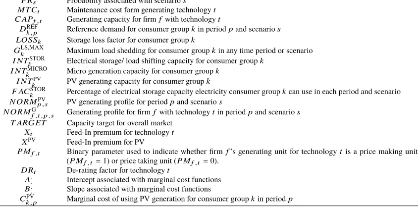
Table 3: Parameters.

PRs Probability associated with scenarios

MT Ct Maintenance cost form generating technologyt

C APf,t Generating capacity for firmfwith technologyt

D_kREF_,p Reference demand for consumer groupkin periodpand scenarios

LOSSk Storage loss factor for consumer groupk

GLS,MAX_k Maximum load shedding for consumer groupkin any time period or scenario

I NTSTOR

k Electrical storage/ load shifting capacity for consumer groupk

I NT_kMICRO Micro generation capacity for consumer groupk I NTPV

k PV generating capacity for consumer groupk

F ACSTOR_k Percentage of electrical storage capacity electricity consumer groupkcan use in each period and scenario

N OR MPV

p,s PV generating profile for periodpand scenarios

N OR MG_f,t,p,s Generating profile for firmfwith technologytin periodpand scenarios T ARGET Capacity target for overall market

Xt Feed-In premium for technologyt

XPV _{Feed-In premium for PV}

P Mf,t Binary parameter used to indicate whether firmf’s generating unit for technologytis a price making unit

(P Mf,t=1) or price taking unit (P Mf,t=0).

DRt De-rating factor for technologyt

A.. Intercept associated with marginal cost functions

B._. Slope associated with marginal cost functions

CPV

k,p Marginal cost of using PV generation for consumer groupkin periodp

Table 4: Functions. CGEN

t (.) Marginal cost function for technologyt

CLS

k,p(.) Load shedding operational cost for consumer groupkin periodp

CMICRO

In this section, the methodology is presented. We utilise a stochastic MCP to represent an

electricity market with two types of players: generation firms and electricity consumer groups. The

model is similar to the model developed in Bertsch et al. (2018) but with the following differences:

1. Generation firms may be modelled as either price-takers or price-makers, i.e., the model can

incorporate market power.

2. We only consider operational decisions and do not consider investment and decommissioning

decisions. This is because the focus of the paper is to understand how operational decisions on

the demand side, such as load shifting and micro-generation, can mitigate market power on the

supply side.

Firms receive revenues from energy and capacity markets as well as a FIP and seek to

maximise profits. As in Bertsch et al. (2018), the capacity payment mechanism we consider is a

quantity based mechanism. Firms may hold multiple generating units of baseload, mid merit, peakload

and wind technology. They are distinguished by the generation portfolio they hold and by the ability

to exercise market power.

On the demand side, we consider a number of different consumer groups, including

commercial/industrial as well as residential consumers. Consumers minimise the cost of meeting

their demand. They do so by utilising a range of possible demand-side flexibility measures, such

as load shedding, load shifting, PV generation or thermal micro-generation. We do not model

individual consumers but rather consider different consumer groups, in a similar manner to that

outlined in Bertsch et al. (2018), whose decisions represent the aggregate actions of consumers

in these groups. Consumer groups are distinguished by different levels of demand-side flexibility

capability, by their demand profiles and by the ability to self-generate electricity through PV modules

or thermal micro-generation.

The stochasticity of the model arises from the uncertainty surrounding wind and PV power.

Thus, each scenario in our model corresponds to different RES generation profiles, i.e. varying levels

of wind and solar power availability at each point in time, which are correlated, both temporally and

spatially (Bertsch et al., 2018).

Each of the generation firms and consumer groups considered have separate optimisation

problems that are connected through market clearing conditions. The stochastic MCP is made

up of these market clearing conditions along with the Karush-Kuhn-Tucker (KKT) conditions for

simultaneously and in equilibrium.

Throughout this section the following conventions are used: lower-case Roman letters indicate

indices or primal variables, upper-case Roman letters represent parameters (i.e., data, functions),

while Greek letters indicate prices or dual variables. The variables in parentheses alongside each

constraint in this section are the Lagrange multipliers associated with those constraints.

2.1 Firm f’s problem

Firm f maximises its expected profits (revenues less cost) by choosing the amount of generation, the

quantity of capacity bid. Firm f considers revenues received from a capacity and an energy market

as well as a FIP for RES generation. Its costs consist of generation costs and any costs incurred for

maintaining its units.

Firm f’s optimisation problem is:

max

genf,t,p,s,capbidf,t,

exitf,t

Õ

t,p,s

PRs×genf,t,p,s× γp,s+Xt−CtGEN(genf,t,p,s)

−

Õ

t

C APf,t×MTCt+

Õ

t

DRt×κ×capbidf,t,

(1a)

subject to:

genf,t,p,s ≤C APf,t×NORMGf,t,p,s, ∀t,p,s, (λ

1

f,t,p,s), (1b)

capbid_f,t ≤C APf,t, ∀t, (λ2_f,t), (1c)

where the marginal cost of generating with technologytis

C_tGEN(x) = AGEN_t +BGEN_t x, (2)

which means the overall cost of generating electricity with technologytis quadratic. Constraints (1b)

and (1c) constrain the amount of energy generated by and the capacity bid of firm f. In addition, each

of firm f’s primal (decision) variables are also constrained to be non-negative.

The capacity price paid for each unit of capacity bid accepted isκ. It is exogenous to firm

f’s problem but is a variable of the overall problem, determined via the market clearing condition

variables cannot affect this price (i.e., ∂γp,s

∂genf,t,p,s =0). In this case,γp,sis exogenous to firm f’s problem but is a variable of the overall problem, determined via the market clearing condition (8a).

If firm f’s generating unit for technologytis assumed to be a price-maker unit, then its generation

decision variable for that unit (genf,t,p,s) can affect the energy price. As a result, we derive the

following relationship between the energy price and generation:

genf,t,p,s=

Õ

k

DREF_k,p +gup

k,p,s−LOSSkg

down

k,p,s−g

pv

k,p,s

−Õ

k

γp,s−ALS_k,p+µ_k1_,p,s+µ8_k,p,s

B_kLS_,p

−Õ

k

γp,s−AMICRO_k,p +µ_k4_,p,s+µ8_k,p,s

B_kMICRO_,p

−

Õ

ˆ

f,t

γp,s+Xt−AGENt +λ1_fˆ_,t,p,s

BGEN_t

+γp,s+Xt−A

GEN

t +λ1f,t,p,s

B_tGEN ,

(3)

where the parameters and variables not mentioned already are parameters and variables from the

consumers’ problem (section 2.2) and hence exogenous to firmf’s problem. Equation (3) is determined

by combining market clearing condition (8a) with the KKT conditions that determine how consumers

shed their load (10a), utilise micro-generation (10d), and the KKT conditions that determine how

firms generate (9a) (all except firm f’s unitt). The remaining KKT conditions cannot be used as they

cannot be substituted into (8a). For price-making firms, this relationship is substituted into firm f’s

objective function (1a) leading to

∂γp,s

∂genf,t,p,s

=−

1 Í

k _2B1LS

k,p

+_Í 1

k _2BMICRO1

k,p

+ 1

(Í

ˆ

f,t 2B1GEN

t

) − 1

2BGEN

t

. (4)

Equation (4) represents firm f’s conjectural variation of how it believes it can influenceγp,swith its

generation decisions. If firm f is a price-taker, then its problem is convex assumingB_tGEN∀t. If firm

f’s generating unit for technologytis a price-maker, then its problem is strictly convex, assuming

B_tGEN>0,BLS_k,p >0, andBMICRO_k,p >0,∀k,p,t.

The firms’ KKT conditions are presented in appendix A.1. Note: PMf,tis a binary parameter

that is used in the KKT conditions to indicate whether firm f’s generating unit for technologytis a

2.2 Consumer groupk’s problem

Consumer groupk’s optimisation problem is the same as that presented in Bertsch et al. (2018)

where each consumer group minimises the cost of meeting their expected demand. As part of their

optimisation problem, they may choose to (partially) shed their load or to (partially) self-generate

using solar PV or thermal micro generation. For PV generation, they receive a FIP. Consumer group

kmay also shift some of their demand and obtain less from the grid. We consider shifting in the same

way as electrical storage where consumers may obtain electricity from electrical storage.

Consumer groupk’s optimisation problem is:

min

gls

k,p,s,g

up

k,p,s,g

down

k,p,s,

gmicro

k,p,s,g

pv

k,p,s Õ

s,p

PRs

γp,s× DREFk,p −gkls,p,s+g

up

k,p,s− (1−LOSSk)g

down

k,p,s−g

micro

k,p,s−g

pv

k,p,s

−XPV×gpv_k,p,s+g_kls_,p,s×C_kLS_,p(g_kls_,p,s)+g_kmicro_,p,s×C_kMICRO_,p (gmicro_k,p,s)+g_kpv_,p,s×C_kPV_,p

(5a)

subject to

gls_k,p,s ≤ GLS,MAX_k , ∀p,s, (µ1_k,p,s), (5b) gup_k,p,s ≤ F AC_kSTOR×I NT_kSTOR, ∀p,s, (µ2_k,p,s), (5c) gdown_k,p,s ≤ F AC_kSTOR×I NT_kSTOR, ∀p,s, (µ3_k,p,s),(5d) gmicro_k,p,s ≤ I NT_kMICRO, ∀p,s, (µ4_k,p,s), (5e) gpv_k,p,s ≤ NORM_pPV_,s×I NT_kPV, ∀p,s, (µ5_k,p,s), (5f)

p0+h−1

Õ

e=p0

gup

k,e,s−g

down

k,e,s

≤ I NT_kSTOR, ∀s,p0,h, (µ6_k,p0_,h,s), (5g)

p0_+h−1

Õ

e=p0

gdown_k,e,s−gup

k,e,s

≤ 0, ∀s,p0,h, (µ7_k,p0_,h,s), (5h)

gls_k,p,s+(1−LOSSk)gdownk,p,s+g

micro

k,p,s+g

pv

k,p,s ≤ D

REF

k,p +g

up

k,p,s, ∀p,s, (µ

8

k,p,s), (5i)

The marginal cost functions associated with load shedding and micro generation are:

C_kLS_,p(x) = ALS_k,p+B_kLS_,px, (6)

Constraint (5b) limits the amount of electricity consumer group k can shed. Similarly,

constraints (5c) and (5d) limit the amount of their demand they increase and decrease, respectively,

i.e., these constraints limit the amount of electricity they can shift/store. Constraints (5e) and (5f)

limit the amount of electricity consumer groupkcan self-generate from micro- and PV generation,

respectively.

Constraint (5g) ensures consumer group kcannot, over a|H|-timestep period, store/shift

more electricity than its storage capacity. Constraint (5h) ensures consumer groupkcannot, over

the same |H|-step time period, use more electricity for meeting demand than what has already

been stored/shifted. Constraints (5g) and (5h) also ensure that any electricity stored/shifted in a

|H|-timestep period cannot be used in any other|H|-timestep period. In Section 4, we set|H|=48 as

we believe this storage (load shifting) horizon is reasonable given the daily trough and peak structure

of electricity demand.

Constraint (5i) ensures any electricity generated by consumer group kmust be less than

their reference demand (the demand consumers have in absence of any demand side flexibilities). In

other words, constraint (5i) ensures consumer groupk’s own generation cannot be used to meet other

consumers’ demand.

Consumer group k’s problem is convex, assuming all values for BLS_k,p and BMICRO_k,p are non-negative. Its KKT conditions are the same as those presented in Appendix A.2 of Bertsch et al.

(2018).

2.3 Market clearing conditions

The optimisation problems of each player are connected via the following market clearing conditions:

Õ

f,t

genf,t,p,s=

Õ

k

DREF_k,p −g_kls_,p,s+g_kup_,p,s−LOSSkgkdown,p,s−g

micro

k,p,s−g

pv

k,p,s

_,

∀p,s, (γ_p,s), (8a)

Õ

f,t

DRt×capbid_f,t =T ARGET, (κ), (8b)

Market clearing condition (8a) ensures that the total amount of electricity generated by the firms must

equal the sum of the consumers’ demand. Consumers’ demand consists of their reference demand

demand represents consumers’ demand in the absence of any demand response. Equation (8b) ensures

that the sum of capacity bids from firms, times a derating factor1, must equal the capacity target.

Assuming each of the players’ optimisation problems are convex, the KKT conditions are

both necessary and sufficient for optimality (Gabriel et al., 2012). Thus, the stochastic MCP consists

of the KKT conditions of all players in addition to the market clearing conditions. The problem is

solved in GAMS using the PATH solver.

3. MODEL INPUTS

In the previous section we presented the MCP used in this work. In this section, we describe the

model’s input data. As our case study considers the future Irish power system, we base our data

for 2025 on EirGrid (2017). Firstly, in section 3.1, we describe the demand-side data. Secondly, in

section 3.2, we present the conventional supply side data while, finally, in section 3.3, the renewable

generation data is considered.

3.1 Demand side data

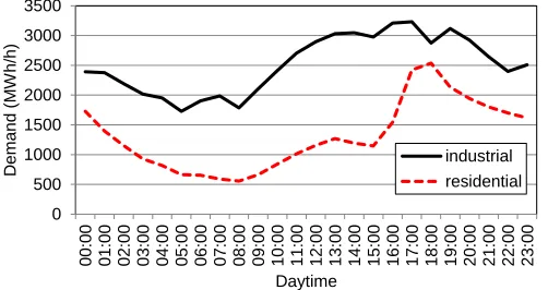
The consumer groups considered in this work include residential consumers in addition to

com-mercial/industrial consumers. Figure 1 displays the reference demand (DREF_k,p) of the industrial and residential consumer groups on a typical day. It shows that the residential demand profile has a peak

that is more pronounced than the industrial one. Based on EirGrid (2017), we assume total annual

electricity demand of 33.6 TWh and peak demand of 5655 MW.

0 500 1000 1500 2000 2500 3000 3500 00 :00 01 :00 02 :00 03 :00 04 :00 05 :00 06 :00 07 :00 08 :00 09 :00 10 :00 11 :00 12 :00 13 :00 14 :00 15 :00 16 :00 17 :00 18 :00 19 :00 20 :00 21 :00 22 :00 23 :00 D emand (M W h/h) Daytime industrial residential

Figure 1: Reference demand of industrial and residential consumers on a typical day

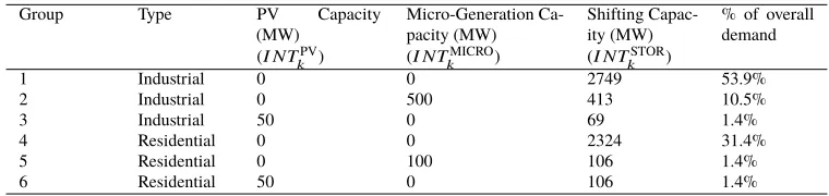
In total, we consider six different consumer groups, three residential and three

cial/industrial. The difference between the groups is in the amount of installed micro-generation and

PV capacity they hold, as described by Table 5. For the different test-cases analysed in section 4, we

consider micro-generation capacities that are 0%, 33%, 67% and 100% of the values presented in

Table 5, which corresponds to 0%, 3%, 7% and 10% of the system level peak demand, respectively.

For PV generation, the installed capacities remain fixed across the test cases.

Table 5: Consumer group characteristics.

Group Type PV Capacity

(MW)

Micro-Generation Ca-pacity (MW)

Shifting Capac-ity (MW)

% of overall demand

(I NTPV

k ) (I NT

MICRO

k ) (I NT

STOR

k )

1 Industrial 0 0 2749 53.9%

2 Industrial 0 500 413 10.5%

3 Industrial 50 0 69 1.4%

4 Residential 0 0 2324 31.4%

5 Residential 0 100 106 1.4%

6 Residential 50 0 106 1.4%

Each consumer group can shift their load and Table 5 displays the total amount they can

decrease their demand by over a 48-hour period, without increasing again it in that same time horizon.

These values are taken from Bertsch et al. (2018). The percentage values of these capacities each

consumer group can shift in each individual hour (F AC_kSTOR) varies from 0% to 20%. Following Nolan et al. (2017), we assume the quantity target for the capacity market is 1.2 times the system peak

demand, i.e.T ARGET =1.2×5655 MW=6786 MW.

3.2 Conventional power generation data

On the supply side, we consider five power generating firms with different generation portfolios. These

include specialised baseload, mid merit, peakload and renewable firms in addition to an integrated

firm with generation capacity across all of these technologies. Based on EirGrid (2017), the maximum

capacities by technology and firm are presented in Table 6.

Table 6: Maximum geneartion capacity (MW) by firm (C APf,t).

Technology firm 1 firm 2 firm 3 firm 4 firm 5

Existing baseload 900 200 - -

-Existing mid merit 800 - 1250 -

-Existing peakload 200 - - 500

-New baseload 750 - - -

-New mid merit 500 - 800 -

-New peakload 300 - - -

-Wind 2400 - - - 2400

The firms’ optimisation problems considers quadratic cost functions for the conventional

generators as described in section 2.1. In other words, the marginal costs at the intercept increase

Grigg, 1996).

To derive marginal power generation costs at the intercept, we follow Bertsch et al. (2018)

and assume power plant efficiencies of 30% for existing baseload generators, 50% for existing mid

merit generators and 32% for existing peakload generators2. To calculate marginal costs of the new

technologies at the intercept, we assume efficiencies of 45% for baseload, 60% for mid merit and

40% for peakload. The marginal costs in Table 7 were calculated using gas, coal and CO2 prices

of the corresponding futures markets for 2017 as obtained from the European Energy Exchange

(www.eex.com). For this purpose, we used the average market results of the futures markets for 2017

as traded during 2016. Coal and CO2prices are used to calculate variable generation costs of baseload

generation, while gas and CO2prices are used for determining the variable costs of peakload and mid

merit generation, i.e., peakload generators are assumed to be open cycle gas turbines while mid merit

generators are assumed to be combined cycle gas turbines (CCGT).

Table 7: Techno-economic input data of supply side technologies.

Technology Fixed O & M costs Marginal power gen. costs

at intercept

Spec. CO2emissions

(e/MW y) (e/MWhel) (t CO2/MWhel)

(MT Ct) (AGENt )

Existing baseload 41,667 49 1.17

Existing mid merit 27,778 41 0.36

Existing peakload 23,148 63 0.56

New baseload 41,667 32 0.78

New mid merit 27,778 34 0.30

New peakload 23,148 51 0.45

3.3 Renewable power generation data

The variable sources of renewable electricity generation considered in this paper are wind and solar PV.

As with Bertsch et al. (2018) and Lynch et al. (2019), data from the MERRA2 reanalysis (Bosilovich

et al., 2016) were used to generate input data for these two sources. Note that wind and solar PV are

not only variable but also uncertain and their uncertainties are correlated since both depend on the

meteorological conditions. Therefore accounting for these correlations is important when providing

input data for the stochastic MCP.

The analysis is based on hourly MERRA2 data on surface incoming shortwave flux, wind

speed and air temperature for the years 1981 to 2015 inclusive. This data was transformed to wind and

solar capacity factors. For solar PV, the transformation follows Ruppert et al. (2016) and Schwarz et al.

(2018) using parameters for Ireland, described in Bertsch et al. (2017). For wind, the transformation

is based on the method from Cradden et al. (2017) and Cannon et al. (2015) and the wind speed to

capacity factor curve by Ofgem (2013). For computational reasons, the hourly wind and solar capacity

factor time series of 35 years were then clustered into six representative years.

Details of the renewable data generation and the clustering procedure are described in Bertsch

et al. (2018) while the probabilities and chosen years of occurrence are summarised in Table 8. To

ensure that the spatial and temporal correlations between wind and PV are preserved, we use these

historical wind and PV data as a basis for our analysis. As Table 5 indicates, we consider 50 MW

of solar PV capacity, which are installed on the demand side. Furthermore, Table 6 shows that we

consider 4800MW of installed wind capacity. We base these assumptions around installed RES-E

capacity estimates for 2025 from EirGrid (2017).

Table 8: Representative years chosen for RES scenarios and corresponding probabilities of occurrence (see Bertsch et al., 2018).

Year 1983 1998 2001 2003 2004 2015

Probability of occurrence 0.486 0.286 0.086 0.086 0.029 0.029

We assume a FIP payment ofXt =XPV= 23e/MWh for wind and PV generation. These

values are obtained from Farrell et al. (2017). A FIP is not considered for any other technology. For

both wind and solar we assume a marginal generating cost of zero.

4. RESULTS

In this section, we present the results of our work, focusing on how DR can help mitigate the impact

of MP on consumer costs, firms’ profits and emission levels. As described in the previous section,

we exogenously vary the amount of installed micro-generation capacity consumers have and the

percentage of their total load shifting capacity they can use in each hour. In addition, we also consider

test cases where the market is perfectly competitive, i.e., all players are price takers, and test cases

where market power is present. For the cases with market power, we consider an oligopoly with

a competitive fringe. The price making oligopolists are the integrative firm and the specialised

mid-merit firm. The price taking competitive fringe includes firms 2, 4 and 5.

When describing the results, we focus on load shifting and its interactions with

micro-generation. While consumers are also capable of shedding their load, as described in the previous

section, the results show minimal amounts of this behaviour. In the perfect competition cases, we

see no load shedding throughout the market. In the market power cases, residential consumers also

consumers choose to shed is 2.7MWh in a particular peak hour. These results can be explained by

the capacity portfolio considered in this case study, which is large enough to meet consumers peak

demand. Consequently, we do not concentrate on load shedding in the results to follow.

This section is organised as follows: in section 4.1 we present the consumer costs results

whereas in section 4.2 we describe the results in relation to the generating firms’ profits. Finally, in

section 4.3, the emissions results are presented.

4.1 Consumer costs

Figure 2 displays expected consumer cost (weighted average by demand) for each of the consumer

groups in the absence and presence of market power for different levels of load shifting and

micro-generation capacity. These values are calculated using equation (5a) and by dividing by each group’s

total yearly demand. When market power is present in the market, Figure 2 shows that costs increase

substantially for each of the consumer groups and that DR can generally help mitigate against these

effects.

More specifically, increasing the amount of micro-generation in the market decreases the

costs for each group. This is despite the fact that only consumer groups 2 and 5 have micro-generation

capacity. These results suggest that micro-generation can help restrict generation firms’ ability to exert

market power and thus benefit all consumer groups even if they do not hold such capacity themselves.

Figure 2 also shows that, while there are noticeable differences between the 0MW, 200MW and

400MW cases, there is little difference between the 400MW and 600MW cases, in terms of consumer

costs. This suggests that once a significant amount of micro-generation is installed on the system

(400MW in this case), the marginal benefits of micro-generation decrease.

As for load shifting, Figures 2a, 2b, 2e and 2f show that, in the presence of market power,

shifting can also reduce costs of consumers, particularly of those without their own micro-generation.

This holds for industrial consumer groups 1 and 3 in addition to residential consumer groups 4 and 6,

and regardless of the level of micro-generation in the system. The relative cost decrease, from 0% load

shifting to 20%, is greater for residential consumers than industrial consumers. The percentages are

6%, 7%, 10% and 12% for groups 1, 3, 4 and 6, respectively (assuming 600MW of micro-generation).

These results can be explained by the consumers’ load curves (Figure 1) and the price duration curves

(Figure 3b). Residential consumers’ peak demand is far more pronounced than that of industrial

(a) Consumer group 1 (Industrial, w/o PV, w/o Micro-gen)

(b) Consumer group 4 (Residential, w/o PV, w/o Micro-gen)

(c) Consumer group 2 (Industrial w Micro-gen) (d) Consumer group 5 (Residential w Micro-gen)

(e) Consumer group 3 (Industrial w PV) (f) Consumer group 6 (Residential w PV)

For consumers with their own micro-generation, Figures 2c and 2d show that load shifting

can also help reduce their costs. However, this is only when these consumers have low levels of or no

micro-generation. When consumer groups 2 and 5 have 400MW of micro-generation installed, these

results show that load shifting does not reduce their costs anymore. In fact, for industrial group 2,

load shifting slightly increases their costs, when 600MW of micro-generation and market power are

present. These lacks of reduction can be explained by the fact that micro-generation only becomes

profitable to utilise when prices are high. Consequently, when prices are high, micro-generation

reduces consumer costs without the need to increase off-peak prices and costs, which is in contrast to

load shifting.

Comparing load shifting and micro-generation as to how they can help mitigate against

the consumer cost increase resulting from market power, our findings show that these technologies

compensate one another, i.e. the effect of load shifting decreases when the level of micro-generation

in the system increases and vice versa. Moreover, we find that the relative effects of micro-generation

and shifting generally have a similar magnitude (varying between 6-14%), where micro-generation

has a slightly higher relative cost reduction effect for industrial consumers, whereas shifting has a

slightly higher effect for residential consumers. This finding holds except for the consumers that have

their own micro-generation (i.e. consumer groups 2 and 5). For these two consumer groups, the

relative cost reduction of micro-generation in the presence of market power is significantly higher

(varying between 25-35%), whereas the relative effect of shifting is lower (0-8%).

Moreover, Figure 2 also shows that consumers with installed PV capacity (groups 3 and 6)

have smaller expected average costs when compared with consumers with no PV or micro-generation

(groups 1 and 4). This holds regardless of the level of micro-generation, load shifting or market

power presence in the overall market. It also holds when we compare residential groups 5 and 6.

Likewise, when industrial groups 2 and 3 are compared, we observe similar results when there are

0MW and 200MW of micro-generation and when there is no market power present in the market.

However, in contrast, when there are 400MW and 600MW of micro-generation and market power

in the market, group 2 has lower average costs than group 3. This can be explained by the fact that

PV and peak demand are negatively correlated. Thus, in peak demand time periods, intermittent PV

generation is less likely to be able to meet demand. In contrast, micro-generation is most beneficial to

consumers in such high demand time periods. This finding suggests that relatively large amounts of

micro-generation are superior to PV in reducing the high prices resulting from market power.

(a) Total expected consumer costs (b) Price duration curve (600MW of micro-generation)

Figure 3: Total consumer costs and price duration curves, with (MP) and without (No MP) market power.

objective functions. As mentioned above, it generally shows that both load shifting and

micro-generation can help reduce consumer costs, hence contribute to mitigating the impact of market

power on consumers. Despite this, it is also important to note, that even when there is 600MW of

installed micro-generation and consumers are able to shift 20% of total shifting capacity in each hour,

consumer costs are still significantly higher than in the perfect competition case.

On a side note, in a perfectly competitive market, load shifting slightly increases the expected

costs of industrial consumers (groups 1-3), which is in contrast to the findings for the imperfect

competition case discussed previously. For residential consumers, however, load shifting also leads to

a slight cost reduction when there is no MP present. These differences can again be explained by

the relatively flatter nature of industrial consumers’ demand (see Figure 1). In addition, Figure 3b

shows that, in the absence of MP, the decrease in peak prices caused by load shifting is not as big as

the increase in off-peak prices, which is in contrast to the imperfect competition case. Consequently,

because their demand is relatively flatter, industrial consumers do not reap the benefits of load shifting,

in the absence of market power. In fact, their costs increase as a result of the residential consumers’

shifting.

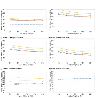
4.2 Firms’ profits

Figure 4 displays the expected profits for each of the generating firms, as described by equation (1a).

When market power is present in the market, Figure 4 shows that each firms’ expected profits increase

substantially. This is despite the fact that only firms 1 and 3 have the ability to exert market power.

In the market power cases, firm 1 and 3 reduce the generation they would otherwise provide to the

market. This allows/forces more expensive generating units of these and other firms to come online

(a) Firm 1 (Integrated firm) (b) Firm 2 (Baseload firm)

(c) Firm 3 (Mid merit firm) (d) Firm 4 (Peakload firm)

(e) Firm 5 (Wind only firm, market power cases) (f) Firm 5 (Wind only, no market power case)

Similar to the effects described in section 4.1, Figure 4 generally shows that DR can help

mitigate the impact of market power. More specifically, when market power is present, increasing

the amount of micro-generation in the system reduces expected profits for each of the five firms.

This holds regardless of the level of load shifting. Micro-generation allows consumers to reduce the

demand they place on the firms, which reduces firms 1 and 3’s price-making ability and, consequently,

system prices. However, Figure 4 shows that this decrease in firms’ profits becomes minimal when the

consumers increase the amount of micro-generation from 400MW to 600MW. As above, this results

suggests a saturation effect in micro-generation’s ability to reduce the effects of market power.

As for load shifting, Figures 4a - 4d show that, in the presence of market power, shifting

decreases expected profits for firms 1 - 4 respectively. This holds regardless of the level of

micro-generation in the market. Firms’ ability to exert market power is strongest at times of high demand.

Load shifting allows consumers to decrease their peak demand, which reduces the price-making

ability of firms 1 and 3 and, consequently, prices and profits.

In contrast, Figure 4e shows that the renewable only firm’s expected profits initially increase

as a result of load shifting being introduced into a market where market power is present. As with

the perfect competition cases, this is because load shifting increases off-peak demand and prices

and decreases wind curtailment. However, as the level of load shifting increases further, Figure 4e

shows that firm 5’s profits turn and start to decrease again. As Figure 3b illustrates, load shifting also

decreases peak prices. This effect is greater when some firms are exerting market power. Thus, the

initial benefits of load shifting from firm 5’s perspective (driven by reduced wind curtailment and

increased offpeak prices) become overshadowed by the reduced peak prices. These results suggest that,

in the presence of market power, relatively small amounts of load shifting can increase the profitability

of renewable generation while larger amounts can reduce this effect. Furthermore, the most favourable

level of load shifting for firm 5 in such a market, depends on the level of micro-generation. For

example, when there is 0MW of micro-generation, the most favourable percentage of load shifting

capacity for firm 5 is 5%, whereas this value is 15% when there is 600MW of micro-generation

present. This can be explained by micro-generation’s ability to mitigate the effects of market power

and reduce peak prices. As the capacity of micro-generation in the system increases, there is less

MP in the system; hence the downside effect of load shifting during peak hours decreases, while the

upside effect during offpeak hours remains. As a result, for larger amounts of micro-generation in the

system, firm 5 only benefits from the positive impacts load shifting brings.

portfolio of wind generation. However, Figure 4 shows its expected profit curves are in contrast to

firm 5’s. Firm 1’s decreasing profit curves are dominated by the reduced profits of its conventional

units, as explained above.

Comparing load shifting and micro-generation as to how they can help mitigate against the

generation firms’ profit increase, our results show that the effect of load shifting decreases when

the level of micro-generation in the system increases and vice versa, i.e. these are compensating

technologies. The relative effects of micro-generation and load shifting on the profits of the specialised

conventional firms generally have a similar magnitude (between 18-23% for baseload generation,

between 20-28% for mid-merit generation and between 31-36% for peakload generation), where

micro-generation has a slightly higher relative profit reduction effect for baseload and mid-merit

generation, whereas there is no clear effect difference for peakload generation. The relative profit

reduction effects are much smaller for the integrated and renewable-only firms, where micro-generation

leads to profit reductions of 12-16% and 5-8% for the integrated and renewable-only firm respectively,

whereas load shifting leads to a relative profit decrease of 5-9% and 0-2% for the integrated and

renewable-only firm respectively.

On a side note, when the market is perfectly competitive, Figures 4b - 4d show that load

shifting has a relatively small impact on profits for firms 2 - 4, respectively. Although not visible in

Figure 4d, firm 4’s expected profits increase slightly as the level of load shifting increases. This is

caused by an increase in capacity prices and the fact that, in the absence of market power, firm 4 only

participates in the capacity market. The price increase in the capacity market is a result of decreasing

profits of conventional generation in the energy market. As we assume a competitive, quantity-based

capacity market, this leads to a capacity price increase, i.e. the capacity market compensates the

reduced profits in the energy market (for further details, see Bertsch et al., 2018). In contrast, firm

3’s expected profits slightly decrease as a result of increasing load shifting, in the absence of market

power. Despite earning increased revenue from the capacity market, this decrease can be explained by

the reduced peak hour energy prices; see Figure 3b. Moreover, as firm 3 is a mid-merit only firm, it

does benefit from the increase in off-peak demand and prices as it is still not profitable for them to

generate in those hours.

In contrast to firms 2 - 4, Figures 4a and 4f show that increasing the percentage of load

shifting capacity from 0% to 10%, increases both firm 1’s and 5’s expected profits in the absence

of market power. This is because firms 1 and 5 are the only firms that have wind generation

Figure 5: Expected emissions and wind generation (600MW of micro-generation).

curtailment and further utilise their wind portfolio. For firm 1, this is despite the reduced profit its

conventional generation units suffer as a result of the reduced peak-hours demand and prices. When

the hourly load shifting capacity increases from 10% to 20%, in the absence of market power, Figures

4a and 4f show that the expected profits of firms 1 and 5 do not increase substantially. This result

suggests that the marginal effect of developing load shifting technologies reduces once there is already

a considerable amount of it present.

4.3 Emissions

Finally, Figure 5 displays the expected levels of emissions and wind generation for different load

shifting cases, both in the presence and absence of market power. The results show that overall wind

generation levels are lower in non-competitive market conditions. This is because, when firm 1 is a

price-making firm, it reduces its wind generation in order to force/allow more expensive generating

units into the market, which are more emission-intensive at the same time. Hence, when price-making

firms own renewable generation, their price-making behaviour can lead to increased system emissions

as a side effect.

Moreover, Figure 5 shows that, as load shifting increases, so does the amount of wind

generation. This result concurs with Lynch et al. (2019) and is because load shifting increases off-peak

demand and thus reduces wind curtailment. However, Lynch et al. (2019) only consider a perfectly

competitive market, whereas Figure 5 shows that the increase in wind generation, as a result of

increases, we observe that emissions do not decrease as the level of load shifting increases when

market power is present. As opposed to the perfect competition case, when firm 1 is able to exert

market power, it does not use wind generation solely to meet the increased off-peak demand resulting

from load shifting. It also utilises its conventional units, in particular its baseload units, which have a

high emission factor. In addition, even if firm 1 only ramps up its baseload units to the minimum

possible extent, this will increase system prices so that firm 2 (the price-taking baseload-only firm)

will dispatch its emission-intensive baseload unit, too. Overall, the increase in baseload generation in

off-peak hours is greater than the decrease seen in peak hours. Consequently, while load shifting

increases wind generation, it can also increase baseload generation, when market power is present.

These findings are in contrast to the perfect competition case. In the absence of market

power, Figure 5 shows that increasing levels of load shifting will not only increase wind generation

(particularly in offpeak hours) and decrease conventional peak generation, but also decrease emissions.

This is because in a perfectly competitive market, the increase in off-peak demand is primarily met by

wind.

To summarise, these results suggest that, while DR may help mitigate the impact of MP on

wind generation, its potential in mitigating against the negative effects of MP on emissions is limited

in the considered case. In a perfectly competitive market, however, DR may also be useful in reducing

emissions.

5. DISCUSSION AND CONCLUSIONS

In this work, we present a stochastic mixed complementarity problem to model an electricity market

characterised by an oligopoly with a competitive fringe. We use the model to investigate the

interactions between demand response and market power. More specifically, applying the model to a

stylised version of the 2025 Irish power system, we examine to which extent DR can help mitigate the

impact of market power on consumer costs, generating firm profits and carbon emissions. Our model

generally distinguishes between load shifting, load shedding and self-generation (micro-generation)

within DR, where we focus on the results for load shifting and micro-generation in this paper. In

relation to the research questions set out in section 1, we can summarise three main findings of our

research.

First, DR can generally help mitigate against substantially increasing costs for all consumer

When comparing load shifting and micro-generation within DR in terms of their contribution to

mitigating against the effects of market power, our findings show that the effect of micro-generation

decreases when the level of load shifting in the system increases and vice versa. Hence, we conclude

that these are competing technologies. In addition, the analysis presented reveals that the relative

effects of micro-generation and shifting generally have a similar magnitude. An exception from this

finding are consumers that own micro-generation themselves. For these consumers, the relative cost

reduction of micro-generation in the presence of market power is significantly higher than that of load

shifting. Despite these benefits of DR, however, it is also important to note that even for the highest

capacities of micro-generation and load shifting considered in this paper, consumer costs are still

significantly higher than in the perfect competition case. At the same time, saturation effects could

be observed for both micro-generation and load shifting, which suggests that the potential of DR in

mitigating against the impact of market power on consumer costs is limited.

Second, in the presence of market power, all firms’ expected profits increase substantially,

despite the fact that only two firms have the ability to exert market power. In this case, DR can

generally help mitigate against the profit increase by generation firms. More specifically, we find that

DR is most effective in mitigating increased profits of peakload generators, followed by mid-merit

and baseload generators. The profits of the renewable-only and integrated firms are less affected by

DR. In addition, the analysis in this paper reveals that, with the exception of peakload generators,

micro-generation turns out to be more effective than load shifting in mitigating profit increases.

Despite the benefits of DR demonstrated in this paper, however, it is important to note that even for

the highest capacities of micro-generation and load shifting considered as part of the case study, the

generation firms’ profits are still significantly higher than in the perfect competition case. At the same

time, the analysis has shown saturation effects for both micro-generation and load shifting, which

suggests that the potential of DR in mitigating against the impact of market power on generators’

profits is limited.

Third, while DR helps increase the level of wind generation in the system, it does not help

reduce emissions in the considered case study when market power is present. When firms dispatch

their assets more strategically, it becomes financially rewarding for them not to fully utilise their wind

units but to also use their carbon-intensive baseload units. This finding is in contrast to the perfect

competition case, where increasing levels of load shifting will not only increase wind generation in

offpeak hours and decrease conventional generation in peak hours, but also decrease emissions. The

wind.

Concerning the impact of DR on consumer costs in the presence of market power, our

estimated total expected consumer costs (see Figure 3a) correspond to annual residential consumer

savings of aboute20-80 per household (assuming approximately 1.5 million households in Ireland).

In the absence of market power, Bertsch et al. (2018) estimate significantly lower savings of around

e2-5 per household and year. The difference of more than a factor of 10 between these two estimates is

related to the value of market power mitigation through load shifting. In other words, when analysing

the value of DR, this difference shows that it is important to consider market power effects and how

DR can help mitigate against these when modelling power markets.

Some of the literature cautions against significant investments in demand response

tech-nologies (Allcott, 2011; Feuerriegel and Neumann, 2016) as the savings may not outweigh the costs.

However, the findings of this work clearly demonstrate how DR can act to mitigate against the negative

impacts that market power can have on consumers. This conclusion aligns well with Zarnikau and

Hallett (2008), Zarnikau (2010) and Walawalkar et al. (2008) who each discuss the benefits of demand

response in relation to increasing electricity market efficiency and competitiveness. Interestingly,

however, this paper also shows that load shifting should not be the only DR technology considered

when seeking how to best mitigate against market power since micro-generation has also proven to

reduce consumer costs reliably. In fact, from the perspective of an individual consumer, owning

controllable micro-generation capacity that can be used for self-generation has been shown to be more

effective than PV-based self-generation or load shifting when it comes to mitigating the impact of

market power.

These findings will be of interest to policymakers who are concerned over market power in

their relevant electricity market, particularly, if their aim is to reduce consumer costs. However, such

policymakers should also note that load shifting does not necessarily decrease carbon emissions when

market power is present. However, while the findings of this paper have clearly demonstrated the

benefits of DR in relation to mitigating market power impacts, the analysis has also shown that DR

alone will not be sufficient to ensure market competitiveness. The finding that micro-generation turns

out to be the most effective technology for mitigating market power in our case study is obviously

driven, at least to some extent, by the model input data. This does not imply automatically that all

consumers becoming self-sufficient would be an efficient way to mitigate market power. What it does

suggest though is that an increasing number of market participants that can provide generation to the

Critically reflecting on our approach, we wish to acknowledge some limitations. While

the model’s data is based on the projected Irish power system for 2025, the case study is stylised in

nature. Furthermore, we do not consider investment decisions by either the generating firms (e.g.,

in new generation) or by the consumers (e.g., in extra PV or micro-generation). In addition, when

determining making ability, we assumed a fixed conjectural variation, i.e. when modelling

price-making firms, we assume that the ratio between these firms’ generation output and the corresponding

influence on energy prices is fixed. Finally, while we do consider uncertain wind and solar profiles,

a rolling-horizon optimisation approach may more accurately reflect operational decision making

(Devine et al., 2016). Future research will seek to address these limitations.

ACKNOWLEDGEMENTS

Devine acknowledges funding from Science Foundation Ireland (SFI) under the SFI Strategic

Partnership Programme Grant number SFI/15/SPP/E3125. The opinions, findings and conclusions or

recommendations expressed in this material are those of the authors and do not necessarily reflect the

views of the Science Foundation Ireland. Bertsch acknowledges funding from the ESRI’s Energy

Policy Research Center. All omissions and errors are our own.

A. KARUSH-KUHN-TUCKER CONDITIONS

This appendix presents the Karush-Kuhn-Tucker (KKT) conditions for optimality for the two types of

players modelled in this work. These conditions, along with the market clearing conditions (8), make

up the mixed complementarity problem. The ‘perp’ notation 0≤a⊥b≥0 is equivalent toa ≥0,

b≥0 anda.b=0.

A.1 Firms’ KKT conditions

0≤genf,t,p,s ⊥ −PRs

γp,s+Xt+PMf,t

∂γp,s

∂genf,t,p,s

Õ

¯

t∈T

genf,t¯,p,s

−

∂CGEN

f,t

∂genf,t,p,s

+λ1

f,t,p,s≥0, ∀f,t,p,s, (9a)

0≤capbid_f,t ⊥ DRt×κ+λ2f,t≥0, ∀f,t, (9b)

0≤λ1_f,t,p,s ⊥ −genf,t,p,s+(C APf,t−exitf,t) ×NORMG_f,t,p,s ≥0, ∀f,t,p,s, (9c)

0≤λ2_f,t ⊥ −capbid_f,t+C APf,t−exitf,t ≥0, ∀f,t. (9d)

A.2 Consumers’ KKT conditions

The consumers’ KKT conditions are

0≤gls_k,p,s ⊥ −PRs γp,s−

∂C_kLS_,p

∂g_kls_,p,s

_+µ1

k,p,s+µ

8

k,p,s ≥0, ∀k,p,s, (10a)

0≤gup_k,p,s ⊥ PRsγp,s+µ2k,p,s+

|H|

Õ

e=p−pˆ+1

µ6

k,pˆ,e,s−µ

7

k,pˆ,e,s

−µ8_k,p,s≥0, ∀k,p,s, (10b)

0≤gdown_k,p,s ⊥ −PR_sγ_p,s+µ3_k,p,s−

|H|

Õ

e=p−pˆ+1

µ6

k,pˆ,e,s−µ

7

k,pˆ,e,s

+(1−LOSSk)µ8k,p,s ≥0,∀k,p,s, (10c)

where

ˆ

0≤g_kmicro_,p,s ⊥ −PR_s γ_p,s−

∂C_kMICRO_,p

∂g_kmicro_,p,s

+µ4

k,p,s+µ

8

k,p,s ≥0, ∀k,p,s, (10d)

0≤gpv

k,p,s ⊥ −PRs γp,s+X

PV_−CPV

k,p

_+µ5

k,p,s+µ

8

k,p,s≥0, ∀k,p,s, (10e)

0≤µ1_k,p,s ⊥ −gls_k,p,s+GLS,MAX_k ≥0 ∀k,p,s, (10f) 0≤µ2_k,p,s ⊥ −gup_k,p,s+F AC_kSTOR×I NT_kSTOR≥0 ∀k,p,s, (10g) 0≤µ3_k,p,s ⊥ −gdown_k,p,s+F AC_kSTOR×I NT_kSTOR≥0 ∀k,p,s, (10h) 0≤µ4_k,p,s ⊥ −gmicro_k,p,s+I NT_kMICRO≥0 ∀k,p,s, (10i) 0≤µ5_k,p,s ⊥ −gpv

k,p,s+I NT

PV

k ×NORM

PV

p,s ≥0 ∀k,p,s, (10j)

0≤µ6_k,p0_,h,s ⊥ − p0_+h−1

Õ

e=p0

gup

k,e,s−g

down

k,e,s

₊

I NT_kSTOR≥0 ∀k,p0,s,h, (10k)

0≤µ7_k,p0_,h,s ⊥

p0_+h−1

Õ

e=p0

gup

k,e,s−g

down

k,e,s

≥0 ∀k,p0,s,h, (10l)

0≤µ8_k,p,s ⊥ −gls_k,p,s− (1−LOSSk)gdownk,p,s−g

micro

k,p,s−g

pv

k,p,s+D

REF

k,p +g

up

k,p,s ≥0 ∀k,p,s. (10m)

REFERENCES

Albadi, M.H., El-Saadany, E., 2008. A summary of demand response in electricity markets. Electric Power Systems Research

78, 1989–1996.

Allcott, H., 2011. Rethinking real-time electricity pricing. Resource and Energy Economics 33, 820–842.

Ambec, S., Crampes, C., 2012. Electricity provision with intermittent sources of energy. Resource and Energy Economics 34,

319–336.

Bertsch, V., Devine, M.T., Sweeney, C., Parnell, A.C., 2018. Analysing long-term interactions between demand response and

different electricity markets using a stochastic market equilibrium model. URL:http://esri.ie. ESRI working paper.

Bertsch, V., Geldermann, J., Lühn, T., 2017. What drives the profitability of household PV investments, self-consumption and

self-sufficiency? Applied Energy 204, 1–15.

Blumsack, S., Perekhodtsev, D., Lave, L.B., 2002. Market power in deregulated wholesale electricity markets: issues in

measurement and the cost of mitigation. The Electricity Journal 15, 11–24.

Borenstein, S., Bushnell, J., 1999. An empirical analysis of the potential for market power in california’s electricity industry.

The Journal of Industrial Economics 47, 285–323.

Bosilovich, M.G., Lucchesi, R., Suarez, M., 2016. MERRA-2: File Specification. GMAO Office Note , 1–73URL:

http://gmao.gsfc.nasa.gov/pubs/office{_}notes. no.9 (Version 1.1).

Burger, S., Chaves-Ávila, J.P., Batlle, C., Pérez-Arriaga, I.J., 2017. A review of the value of aggregators in electricity systems.

Renewable and Sustainable Energy Reviews 77, 395–405.

power generation statistics: A 33 year case study in great britain. Renewable Energy 75, 767 – 778. doi:http: //dx.doi.org/10.1016/j.renene.2014.10.024.

Caves, D., Eakin, K., Faruqui, A., 2000. Mitigating price spikes in wholesale markets through market-based pricing in retail

markets. The Electricity Journal 13, 13–23.

Comission for Energy Regulation, 2014. CER National Smart Metering Programme Smart Metering High Level Design.

Available online:http://www.cer.ie/docs/000699/CER14046%20High%20Level%20Design.pdf.

Cradden, L.C., McDermott, F., Zubiate, L., Sweeney, C., O’Malley, M., 2017. A 34-year simulation of wind generation

potential for Ireland and the impact of large-scale atmospheric pressure patterns. Renewable Energy 106, 165–176.

doi:10.1016/j.renene.2016.12.079.

Dalton, J.C., et al., 1997. Assessing the competitiveness of restructured generation. The Electricity Journal 10, 30–39.

David, A.K., Wen, F., 2001. Market power in electricity supply. IEEE Transactions on energy conversion 16, 352–360.

De Jonghe, C., Hobbs, B.F., Belmans, R., 2012. Optimal generation mix with short-term demand response and wind penetration.

IEEE Transactions on Power Systems 27, 830–839.

Devine, M.T., Bertsch, V., 2018. Examining the benefits of load shedding strategies using a rolling-horizon stochastic mixed

complementarity equilibrium model. European Journal of Operational Research 267, 643–658.

Devine, M.T., Gabriel, S.A., Moryadee, S., 2016. A rolling horizon approach for stochastic mixed complementarity problems

with endogenous learning: Application to natural gas markets. Computers & Operations Research 68, 1–15.

Devine, M.T., Nolan, S., Lynch, M.Á., O’Malley, M., 2019. The effect of demand response and wind generation on electricity

investment and operation. Sustainable Energy, Grids and Networks , 100190.

EirGrid, 2017. All-island generation capacity statement 2017-2026.

Farrell, N., Devine, M.T., Lee, W.T., Gleeson, J.P., Lyons, S., 2017. Specifying an efficient renewable energy feed-in tariff. The

Energy Journal 38, 53–76.

Feuerriegel, S., Neumann, D., 2016. Integration scenarios of demand response into electricity markets: Load shifting, financial

savings and policy implications. Energy Policy 96, 231–240.

Gabriel, S.A., Conejo, A.J., Fuller, J.D., Hobbs, B.F., Ruiz, C., 2012. Complementarity modeling in energy markets. volume

180. Springer Science & Business Media.

Gabriel, S.A., Kiet, S., Zhuang, J., 2005. A mixed complementarity-based equilibrium model of natural gas markets. Operations

Research 53, 799–818.

Good, N., Ellis, K.A., Mancarella, P., 2017. Review and classification of barriers and enablers of demand response in the smart

grid. Renewable and Sustainable Energy Reviews 72, 57–72.

Green, R.J., Newbery, D.M., 1992. Competition in the british electricity spot market. Journal of political economy 100,

929–953.

Grigg, C., 1996. The IEEE reliability test system: 1996, in: Paper 96 WM 326-9 PWRS, IEEE Winter power meeting 1996,