Using Statistical Analysis to Improve Data Partitioning in Algorithms for Data Parallel Processing Implementation

(1)

Theses Thesis/Dissertation Collections

9-2016

Using Statistical Analysis to Improve Data

Partitioning in Algorithms for Data Parallel

Processing Implementation

Manuel E. Hidalgo Murillo [email protected]

Follow this and additional works at:http://scholarworks.rit.edu/theses

This Thesis is brought to you for free and open access by the Thesis/Dissertation Collections at RIT Scholar Works. It has been accepted for inclusion in Theses by an authorized administrator of RIT Scholar Works. For more information, please [email protected].

Recommended Citation

(2)

Using Statistical Analysis to Improve Data

Partitioning in Algorithms for Data Parallel

Processing Implementation

by

Manuel E. Hidalgo Murillo

A Thesis Submitted in Partial Fulfillment of the Requirements for the Degree of Master of Science in Industrial & Systems Engineering

Supervised by

Associate Professor Dr. Rachel Silvestrini Department of Industrial & Systems Engineering

Kate Gleason College of Engineering Rochester Institute of Technology

September 2016

Approved by:

.

Dr. Rachel Silvestrini, Associate Professor

Thesis Advisor, Department of Industrial & Systems Engineering

.

Dr. Katie McConky, Assistant Professor

(3)

Thesis Release Permission Form

Rochester Institute of Technology Kate Gleason College of Engineering

Title:

Using Statistical Analysis to Improve Data Partitioning in Algorithms for Data Parallel Processing Implementation

I, Manuel E. Hidalgo Murillo, hereby grant permission to the Wallace Memorial Library to reproduce my thesis in whole or part.

.

Signature

.

(4)

iii

(5)

iv

Acknowledgments

(6)

v

Abstract

Using Statistical Analysis to Improve Data Partitioning in Algorithms for Data Parallel Processing Implementation

Manuel E. Hidalgo Murillo

Supervising Professor: Dr. Rachel Silvestrini Committee Member: Dr. Katie McConky

(7)

vi

List of Figures

2.2.1. Memory Systems for Parallel Programming (Modified from [1]) . . 6 2.2.2. SPMD Life Cycle (Modified from [11]) . . . 7 3.2.1. Flow diagram to apply the proposed data partitioning method in

data parallel-processing implementation . . . 19 4.1.1. Illustrations of the simulated Ice-Cream Store . . . 31 4.1.2. Interaction plots for the effect of two-level interactions on the

execution time of the Ice-Cream Store Simulation . . . 36 4.1.3. Node Utilization: Ice-Cream Store Simulation . . . 41 4.1.4. Node Utilization Excluding Equal Data Partitioning Approach:

Ice-Cream Store Simulation . . . 42 4.1.5. Simulation-run Execution Times per Node: Ice-cream Store

Simulation . . . 43 4.1.6. Simulation-run Execution Times per Node Excluding Equal Data

Partitioning Approach: Ice-cream Store Simulation . . . 44 4.1.7. Total Execution Times: Ice-cream Store Simulation . . . 45 4.1.8. Total Execution Times + Training Period: Ice-cream Store

Simulation . . . 47 4.1.9. Equal Sized Data Partitioning: Ice-cream Store Simulation . . . 48 4.1.10 Node Utilization: Equal Sized Data Partitioning - Ice-cream Store

Simulation . . . 49 4.2.1. Manufacturing Cell Simulation System. Retrieved from [8] . . . 50 4.2.2 Interaction plots for the effect of two-level interactions on the

(10)

ix

4.2.4. Node Utilization: Manufacturing Cell Simulation (Excluding Model with Only Main Effects). . . 60 4.2.5. Simulation-run Execution Times per Node: Manufacturing Cell

Simulation . . . 61 4.2.6. Total Execution Times: Manufacturing Cell Simulation . . . 62 4.2.7. Equal Sized Data Partitioning: Manufacturing Cell Simulation . . . 63 4.2.8 Node Utilization: Equal Sized Data Partitioning - Manufacturing

(11)

x

List of Tables

3.2.2.1. Minimum number of runs required to create a two-level fractional design with resolutions III, IV and V based on the number of factors. 23 4.1.1. Variable factors considered for the data partition, in the data

parallel implementation of the Ice Cream Store Simulation example . . . 32 4.1.2. Summary of the main effects linear regression model fit for

preliminary screening of the Ice-Cream Store Simulation. . . 34 4.1.3. Summary of the final model fit for the Ice-Cream Store Simulation . 38 4.2.1. Pattern followed part types in the Manufacturing Cell Simulation

cycle. Retrieved form [8]. . . 50 4.2.2. Variable factors considered for the data partition, in the data

parallel implementation of the Manufacturing Cell Simulation example . . . . 52 4.2.3. Summary of the main effects linear regression model fit for

preliminary screening of the Manufacturing Cell Simulation . . . 53 4.2.4. Summary of final model built for the Manufacturing Cell

(12)

Chapter 1

Introduction

Data parallelism is a form of parallelization of computing where data to be processed has to be distributed across multiple processors, and each process performs the same task on different pieces of the overall data set. The implementation of this type of parallelism is useful when large amounts of data have to be processed, and more than one processing unit is required to warrant high performance.

The data partitioning process refers to the distribution of the data among the processors. The process involves splitting the data set into smaller data partitions or batches. A good initial partition is necessary to ensure high performance [4]. A poor data partition can yield unbalanced workloads in terms of computing, causing long execution times or even a failure of the program.

There are different approaches to managing the data partitioning process. Hash functions and equal sized data partitioning are the most common methods to evenly spread data [10] [15]. However, for large volumes of data, these approaches can yield unbalanced workloads. This research presents a load balancing data partitioning method that can improve performance of data parallel implementations. This document will refer to the problem as the “Parallel Data Partitioning Problem”.

(13)

The goal of the research presented in this thesis is to use statistical analysis to improve data partitioning for data parallel implementation. A poor partition quality can lead to serious performance problems. Inefficient data partitions occur when processing units in the parallel environment have unequal workloads compared to each other. The unfair distribution of workload can be due to the amount or type of data that each node has assigned compared to the time to process each data unit.

The data analysis proposes to improve data partitioning by using statistical methods to sample data and predict processing time for each unit. The time estimations are used to partition the data using a greedy algorithm.

Besides workload distribution, parallel data partitioning also affects aspects of how jobs run in a cluster, such as, the network traffic between processes. Improvements in data partitioning can lead to a more efficient use of resources, better-balanced workloads among the processors and, therefore, a significant improvement in execution performance.

Although, parallel implementation performance also depends on many other important factors including hardware infrastructure, parallel environment configurations, and dynamic load balance techniques. This research is limited to the parallel data-partitioning problem and the opportunities for improvement in performance that a static load balancing data partitioning method can offer.

(14)

Chapter 2

Background Knowledge & Literature Review

This chapter provides a brief introduction of the most relevant computer science concepts required to understand the content of the document. The chapter also defines the technical vocabulary used throughout the research. The concepts covered are Parallel Computing, Computer Clusters, Distribute Data Across Processors, Load Balancing, Data Partitioning and the computer science Partition Problem.

2.1.

Parallel Computing

Parallel computing is not a novel concept. It began almost at the same time that modern computers were created. Parallel computing is a form of computation where the processing of calculations occurs simultaneously, operating on the principle that large problems can often be divided into smaller ones and solved simultaneously.

(15)

2.2.

Computer Cluster

A computer cluster is a set of computers, connected in a network, and combined to work together as a single system. Clusters are beneficial to improve performance in a more cost-efficient method than using a single computer of comparable speed. The components of a cluster usually connect through a fast Local Area Network (LAN).

The cluster used to run the experiments in this research is the Tropos Cluster at Rochester Institute of Technology. Tropos possesses 96 cores, all passing messages with microsecond-scale latency [16]. The nodes in the cluster are connected with InfiniBand, which is a computer high-performance network standard.

In addition, not all processing units in Tropos have the same processing capacity. The variation between processing units can affect the results of the analysis. Therefore, only a set of 20 nodes were chosen within the Tropos Cluster to carry out the experiments. These units are equal processing capacity Intel Xenon Ivytown processors. In order to execute the programs only in that subset of processors "Featured Flags" were added as instructions to the bash scripts. The featured flag instructions are commands that allow the user to select special characteristics of the environment to run the program.

2.3.

Distribute Data Across Processes

(16)

In a distributed memory system, one process cannot directly access the memory space of another process. There are standards to manage these communications by abstracting the physical memory system. Message Passing Interface (MPI) is a standardized library designed to run on virtually any parallel computer without regard to its memory architecture (Distributed Memory, Shared Memory, or a Hybrid), and to facilitate distributed data processing. MPI is used in this research to code the data parallel examples to be used as experiments for the proposed data partitioning method. The MPI library implementation used is OpenMPI [7], which is an SPMD open-source library-implementation. For a deeper explanation of the instructions defined in MPI, refer to the tutorial in [1].

[image:16.612.216.421.75.305.2]

SPMD is a method to implement data parallelism. It is the most common style of parallel programming. In SPMD, multiple autonomous processors execute copies of the same program simultaneously on separate batches, or partitions of the data.

(17)

[image:17.612.133.513.330.549.2]

An SPMD program typically has a lifecycle similar to that of the illustration in Figure 2.3.2. This life cycle works as follows: It starts with the source code that compiles into an executable file. The program splits the data and distributes the batches among the processes. Then, the executable file executes many times, simultaneously in each node, running over the different partitions of the data. Finally, when each process has finished its job, it sends the results to a master process that calculates the combined output and finishes the program. This last step is called “reduce”, and is comparable to the reduce function of MapRedue [3], which is a programming model for processing large data sets with parallel-distributed algorithms on a cluster.

(18)

2.4.

Load Balancing

In parallel programming, load balancing is the process of optimizing the use of computational resources. The purpose is to minimize response time by avoiding work overload in any of the processing units. An unbalanced workload means that some nodes will run their jobs for considerably longer times compared to other nodes in the same implementation. It squanders the parallel programing potential.

There are different approaches to manage the data partitioning for parallel implementations. As mentioned before, the most common approaches are hash functions and equal sized data partitioning. Hash functions consist of creating hash tables to map data units with processors in order to spread data smoothly over a range, and then reorder the dataset after the execution of the program. Equal sized data partitioning consists of making partitions of equal size without regard to the data types or contents.

Data partitioning in data parallel implementations can affect the workload balance of the processing units. The approaches mentioned do not consider that issue. Therefore, better load balancing methods can be applied to improve data partitioning.

(19)

Microsoft Research Silicon Valley and Columbia University [10] presented a more complex static approach for data partitioning and load balancing. What they proposed is a method to automatically generate a data-partitioning plan that can optimize performance without running the program on the actual data set. They created a module that analyses the Execution Plan Graph (EPG) – the ordered set of steps that the computer will execute after the program is compiled – and find the computational complexity of each vertex. This module provides general statistics that are useful to make the data partitioning decisions. The information about the relationship between input data size vs. computational I/O cost is based on compact data representations created from a representative sample set for input data, data summarizations including the number of input records, data size, etc.

They called this module Code Analysis. It runs at the compiling level (after the program is compiled, but before it is executed). After the cost for each vertex of the EPG is calculated, it executes another module called Cost Modeling & Estimation. This module will create an optimized EPG, which is the one executed in the parallel environment.

Sarkar and Hennessy [17] presented another example of data partitioning and load balancing optimization. Similar to the previous example, the authors oriented their research to do changes at compiling level. A computational cost estimation was performed based on the size of the data units, including data types, as well as communication cost involved in the communications between nodes. The last measure is important because their load method is dynamic, which means that the program will re-structure the partitioning on runtime if it is necessary.

(20)

define a proper amount of that partitions; making sure that there are not too many or too few.

A dynamic approach also requires a master node to carry out the data partitioning re-structure in real-time and communicate this to the rest of the nodes. Furthermore, if the dynamic load balancing method works upon request, one master node might not be able to time-efficiently manage all the tasks when there are too many nodes. Schedule tasks upon request means that each node has assigned an initial small partition of data, and it will request for more later in the execution.

A quick test in the Tropos Cluster was designed to illustrate this issue. The test consisted of having a node requesting data from a master node and measuring the time of the transaction. The data transferred in the experiment was a reference-type parameter, which means that both nodes had access to the same block of memory (Shared Memory System), and the message contained a reference to the data. This way, no matter the size of the data transferred, the message size will remain constant. Furthermore, no matter what data is been transferred the time of the transaction will remain approximately the same. The test revealed that a single message communication could take approximately 0.005 sec. In addition, the same experiment revealed that having more nodes requesting data from the master node at the same time increases the time of each transaction. For example, if 50 nodes request data at around the same time, the time of the request can increase in some nodes by 1200%, meaning that some messages took up 0.06 sec. to be processed. Trying the same example again but this time having 200 nodes requesting data at the same time, the time of some of the transactions increased to 0.1 sec. For this reason, a dynamic method for data partitioning like this, for very large amounts of data and/or a very large number of nodes, can run into performance issues.

(21)

mentioned before, this research presents a method for data portioning that is meant to be static. The method improves the data partitioning of data parallel implementations without adding latency or complexity to the parallel computing logic. This research will not address the opportunities for improvement in performance that dynamic load balancing methods can offer.

2.5. Data

Partitioning

This section covers examples of some of the problems that can arise using common methods such as hash functions and equal sized data partitioning [10] [15].

First, in a document entitled BotGraph: Large Scale Spamming Botnet Detection [21], the problem of analyzing huge volumes of data to identify abnormal patterns or activities in network security applications is discussed. In order to achieve the goal of identifying abnormal patterns through distributed data parallelism, the writers implemented two simple hash functions. However, running the algorithms in a 240 machines cluster, analyzing 221.5 GB of raw input-data, and dividing the task into 960 partitions, some performance issues arose. One of the algorithms could not finish within the 6-hour quota allowed by the computer cluster. The second algorithm ran for about 1.5 hours, although, the majority of the nodes finished within a few seconds while one of the nodes lasted more than an hour.

(22)

2.6.

Partition Problem

In computer science, the partition problem is a stated formulation of a problem. It consists of separating a given multiset S of positive integers into subsets; you may put as many or as few numbers as you please in each subset, but the sum of the elements of each subset should be as nearly as equal to each other as possible [10]. It is a NP-complete problem, which means that the problem solution has a non-deterministic polynomial execution time, and it is at least as hard to solve in polynomial time as the hardest NP problem.

The partition problem is the same as the parallel data partitioning, and the algorithms that solve this problem can apply to the proposed data partitioning method. In this situation, instead of splitting a multiset of positive integers, the criteria to partition is expected execution times estimated from a statistical analysis.

A main goal for scientists is to implement an algorithm that can solve the problem in polynomial time. However, the only real solution known is brute force (Trying all possible subset arrangement combinations), which runs with exponential execution time. Nevertheless, there are different alternatives proposed that can approximately solve the problem in polynomial time. For example, Greedy Algorithm and Karmarkar’s Algorithm [6].

The greedy algorithm is the simplest and easiest solution for the partition problem. Additionally, the greedy algorithm will, most of the time, find a solution that is close to optimal. For those reasons, this is the algorithm used in this project to address the data-partitioning problem.

(23)

2.6.1. Brute Force Algorithm

The brute force algorithm consists of testing every possible combination of subsets, and then selecting the combination that has the smallest difference. This means, the one for which the difference in the sum of the elements in each subsets is the smallest.

This Algorithm is the only one that optimally solves the partition problem. However, the computational complexity of the algorithm is exponential. The expected execution time is given by the function f(an_{), where ‘a’ is the time to}

test one partitioning combination and ‘n’ is the number of elements in the dataset that have to be split into the subdomains.

For large amounts of data, this solution can be infeasible, because of the amount of memory required to test all of the possible combinations and the time it could take a computer to run the algorithm.

2.6.2. Greedy Algorithm

Greedy is a simple algorithm based on heuristics that aims to produce evenly or almost evenly matched subdomains. It consists of assigning the greatest numbers of the data set, one for each subdomain, and then iterating them in a descendant order, assigning the next element in the list to the subdomain that has the smallest value. The value of a subdomain is the sum of all its elements.

To illustrate this algorithm, let us analyze this example [6]: Imagine you have 10 numbers in random order and you want to split them into two subdomains S1 and S2.

(24)

There are 23 ways to divide the numbers into two subdomains. If we follow the greedy algorithm, we will start by choosing ‘10’ and ‘9’, which are the two largest numbers in the array, and assigning one to each subdomain.

(2 10 3 8 5 7 9 5 3 2) S1 (10) S2 (9)

The next number, if we count in descendant order, is ‘8’. This number will be assigned to the subdomain S2, because its sum of values so far is 9 while for

the subdomain S1 the sum elements is 10.

(2 10 3 8 5 7 9 5 3 2) S1 (10) S2 (9 8)

Now, the next number in descendant order is ‘7’. The sum of the values for the subdomain S2 is now 17, because we added the ‘8’, but for the subdomain

S1, the sum is still 10. Then we add the number ‘7’ to subdomain S1.

(2 10 3 8 5 7 9 5 3 2) S1 (10 7) S2 (9 8)

The process repeats until there are no more numbers to choose. The solution that we end up with has two subdomains with a sum of values of 27 for each subset, which is a perfectly balanced solution.

S1 (10 7 5 3 2) S2 (9 8 5 3 2)

(25)

Nevertheless, the computational complexity of this algorithm is polynomial, which means the solution can be obtained in a reasonable amount of time.

2.6.3. Karmarkar-Karp Algorithm

Karmarkar and Karp [9] presented this algorithm in 1982. Brian Hayes [6] describes it in his article “The Easiest Hard Problem” as follows:

“It is a "differencing" method: This algorithm involves two phases. First, it reads the left-hand side of the table, and the pairs of numbers are replaced by their difference, deciding they will go into different subsets. In the second phase, it reads up the right-hand side. The partition is constructed from the sequence of differencing decisions. For example, 0 at the bottom of the table is known to derive from the difference of two 2s, which can therefore be inserted, one in each subset. One of the 2s arose as the difference between a 6 and a 4, so those numbers can also be written down, and so on. In the case shown the algorithm finds a perfect partition, but it is not guaranteed always to work.” [6]

(26)

Chapter 3

Research Methodology

The data partitioning method presented in this chapter provides a structure to follow during implementation of data parallel-processing programs. The objective is to make the process as simple as possible to replicate in any data parallel implementation where performance issues arise due to unbalanced workloads among nodes.

Discrete Event Simulation is used as the application of this research. This chapter also presents a brief introduction to this concept.

3.1.

Discrete Event Simulations

Discrete Event Simulations (DES) are computational models of the operation of a system. The interactions of the components in the system are simulated as a sequence of events in time. The goal is to execute a simulation repeatedly to generate statistical information about the system behavior.

The benefit of a DES is that testing a system can be faster and more efficient, by allowing us to improve the processes without having to implement the system physically. For example, to test the functionality of a new designed microchip under different stress conditions [8]. Manufacturing many microchips for testing every time a new design is presented can result in large cash expenses that can be reduced by simulating through software the behavior of the microchip.

(27)

initial configurations of the battlefield. Factors that can be modeled are number of attackers on each side, number of each type of machinery, vehicles, and supplies available at a specific moment, statistical relations between different phenomena such as strength, effectiveness of different types of attacks, and other tuning parameters such as shrinking factor and surrender coefficients [20].

In some cases, a DES has to execute several times, trying different initial configuration sets of factors in order to test the system under all possible real life case scenarios. Following the warfare simulation example, if the DES purpose is to study the battlefield and improve the strategy, it will be desirable to run the simulation under different circumstances.

The time it takes to run the simulation every time can be highly dependent on the initial configuration set of factors. Following the same warfare example, certain initial configurations can lead to a quick victory for one of the opponents (short simulation), while other initial configuration sets can lead to very contested battles (long simulation).

The advantage of using a data-parallel implementation to run the DES is that each execution of the simulation can split into different processors and be executed simultaneously. This reduces the execution time of the program to a fraction of the total. For example, assume that the average execution time for a simulation run is 25 seconds. It would take 75.85 days for a single processor to execute the 218_{possible configuration sets. If the workload were split among}

(28)

As an example of the utility of the proposed data partitioning method, think again about the battlefield simulation. If the program requires simulating 100 battles in 25 nodes, then, each node can execute different battle simulations at the same time. An equal data partitioning approach will be to distribute the 100 battle simulations evenly among the 25 nodes, meaning that each node will simulate 4 battles. However, some intimal configurations of the DES can lead to quick battles with an advantaged victory for one of the opponents, and therefore a small amount of events executed by the program, while other configuration sets can lead to much contested battles and a greater amount of events processed. If it is known beforehand which simulation runs will be short or long battles, based on the original configuration set of the simulation, the data partitioning can be improved to evenly distribute workload among the nodes.

This research uses data parallel implementations of discrete event simulations to show the utility of the proposed data partitioning method. The DES implementations coded as examples for this research are: An Ice-cream Store Simulation [19], and a Manufacturing Cell Simulation [8]. The code is implemented, using OpenMPI, a standardized method to achieve data parallelism, and C++, the programing language. The details of the implementations and the results obtained from each example are presented in Chapter 4.

3.2.

Data Partitioning Method

(29)

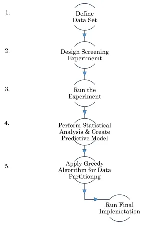
based on selected factors. (5) Use the fit model and the Greedy Algorithm (Section 2.6.2) to create a data partition where the estimated processing times of each subset are nearly equal. (6) Run the final implementation of the data parallel program over the complete data set. Sections 3.2.1 – 3.2.5 contain a detailed explanation for the above steps.

Define Data Set Design Screening Experimemt Run the Experiment Perform Statistical Analysis & Create

Predictive Model

Apply Greedy Algorithm for Data

Partitionng

[image:29.612.137.432.199.649.2]

Run Final Implemetation

Figure 3.2.1- Flow diagram to apply the proposed data partitioning method in

(30)

3.2.1.

Define Data Set

The data set corresponds to a single database table, or data matrix where each column represents a particular variable/factor and each row corresponds to a member or data unit of the data set. In a data parallel implementation, the data set corresponds to the set of data units that is processed by the different nodes of the parallel environment. Each node can process one or more data units.

There are certain requirements that the program and the data set have to meet to apply this data partitioning method. The requirements are:

o The program must be a data parallel implementation. It means that the

parallel program must be of the type SPMD.

o The data should be able to partition into independent data units that run

in separate nodes.

o The time it takes to process a data unit must be, in one form or another,

dependent to the data unit itself. This is to be able to create a predictive model that can estimate the time to process each data unit.

o The program has to run in a cluster with nodes of equal processing capacity.

The variation in the type or capacity of the nodes is not taken into account in the statistical analysis for the proposed method, and this could affect the data partitioning performance.

3.2.2.

Design Screening Experiment

(31)

number of runs and cost to create a predictive model. However, the chosen subset of factor combinations has to be carefully selected to be representative of the overall data set in order to draw statistical conclusion about the execution times.

A screening design can be created by determining a high and a low value for each of the factors in a data unit and carefully selecting few combinations of those factor values. An experimental design of this type is known as two-level fractional factorial design. It is meant to provide accurate knowledge and a high degree of precision of the overall behavior of a system while analyzing a carefully selected subset of observations [5].

For the purpose of this analysis, screening is used to determine what factors or columns in the data units significantly affect the execution time of the program. For example, in a discrete event simulation, with different possible values for each of the factors, the sample data set can be created by choosing a high and a low value for each of the k factors . Different initial configuration sets of these factors can lead the program to process more or less events and execute more or less instructions. The objective then is to create an experimental fractional factorial design; consisting of a carefully chosen subset of factor value combinations to determine which of those factors drive the process and, ultimately, the relationship that exists between those factors and the execution time of the program.

(32)

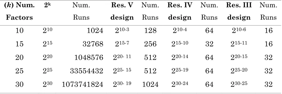
resolutions involve a bigger data sample and, in most cases, it will not add any relevant information for the statistical analysis.

A design with resolution V can estimate the main effects without confounding the effect of other factors and without confounding the effect of two or three level interactions. Resolution V designs can also estimate two-level interaction effects without confounding the effect of other two-two-level interactions. Hence, a resolution V design can be considered a very good option relying on the Sparsity-of-Effects Principle [12], which states that mostly main effects and some low-order interactions determine the relationship from factors to the response.

If there are many factors to be considered, a resolution III design can be used for a quick screening, and determine what of those factors are the most significant. The goal is to move forward in the experiment analyzing only significant factors. A resolution III design can estimate the effect of many factors with an efficient number of runs. However, the estimations made may be confounded with two-level interactions. Nonetheless, a resolution III design in this case is belittled as an initial screening.

(33)

(k) Num. Factors

2k _Num.

Runs Res. V design Num. Runs Res. IV design Num. Runs Res. III design Num. Runs 10 210 ₁₀₂₄ ₂10-3 ₁₂₈ ₂10-4 ₆₄ ₂10-6 ₁₆

15 215 ₃₂₇₆₈ ₂15-7 ₂₅₆ ₂15-10 ₃₂ ₂15-11 ₁₆

20 220 _{1048576 2}20- 11 ₅₁₂ ₂20-14 ₆₄ ₂20-15 ₃₂

25 225 _{33554432 2}25- 15 ₅₁₂ ₂25-19 ₆₄ ₂25-20 ₃₂

30 230_{1073741824 2}30- 19₁₀₂₄ ₂30-24 ₆₄ ₂30-25 ₃₂

In addition, the data sample can be augmented by adding or repeating combinations of factor values to account for variability in the execution of the program. The design can also be improved by adding center points to the high/low values to test for curvature in the relationship between factors and execution time. However, as mentioned before, enlarging the sample data will also increase the time it takes to run the program and gather the execution times to create the predictive model.

For the purpose of this research, the sample data created for both application examples do not include repetitions or center points. However, since the relationships from factors to the execution times are almost perfectly linear and the processing units in the parallel environment are selected to have the same processing capacity, the models created are still very good at estimating execution times.

3.2.3.

Run the Experiment

After having defined the experimental plan, run the parallel program in the cluster and gather the execution times associate with processing each data unit. The objective is to gather the times to have a sampling of the data for a

Table 3.2.2.1- Minimum number of runs required to create a two-level

[image:33.612.86.537.134.285.2]

(34)

statistical analysis. The program can only be run in one node of the cluster. This will sidestep the need of partitioning the data without yet having a data partitioning method implemented. Furthermore, running the program in only one node will elude nuisances that small differences in the processors can add to the execution time measurements.

Gather the execution times by measuring the time between the moment that the program starts processing each data unit and right before it is processed. This is the execution time associated with processing each data unit. Make sure not to time extra-instructions executed by the program that are not associated to processing a data unit itself. It can add nuisance to the measurements and affect the statistical analysis.

At this point, it is possible to see if the proposed data partitioning method will improve the performance of the parallel implementation by looking at the differences in the time to processes each data unit. Large differences in those times are a sign that a better partition can be performed rather than a common hash function or equal sized data partition.

3.2.4.

Perform Statistical Analysis and Create Predictive Model

With the data gathered from the previous step, it is now possible to build an accurate statistical model. The objective of the model is to generate estimations of the time it takes to process each data unit in the cluster based on the factors associated to the same data unit.

(35)

times is almost perfectly linear. A regression model is ideal when the relationship between the variables can be defined by a linear equation.

As it has been mentioned before, the factors used in this research for the statistical analysis are factors in the data units that are thought to affect the execution time. Using discrete event simulations to show an example, these factors are the different real world assumptions that change from one simulation run to another. For example, the arrival rate of entities into the system, system capacity, etc. The differences in execution times are due to different initial configuration sets leading the program to run different amounts of events in each simulation run. Examples of events in a discrete event simulation are entities entering the system, processing an entity in a server or pulling out entities from waiting queues. The amount of events executed by each simulation run is dependent on the initial configuration set of the factors. The statistical analysis performed in the proposed data partitioning method is based on this dependence.

Nevertheless, not every factor has a significant influence in the processing time of the data units nor all factor interactions (the compounded effect of the combinations of factors over the processing time of the data unit). Furthermore, if a model is created including every factor and low-level interactions, it can make the model excessively complex and over fitted. This issue can lead to poor predictive performance. For example, in the ice cream simulation presented in Chapter 4, the simulation has 18 factors. A model including all the simulation factors and two-level interactions – the compounded effect of each pair combination of factors over the processing time of the data unit – will be a model with 324 variables. In the manufacturing cell simulation example, with 26 factors, the model can contain 676 variables. For this reason, it is important to make a careful selection of the factors that will be included in the model.

(36)

to the optimal adjustment. A preliminary screening analysis can help to start drawing what are the main factors and interactions to make a wise selection of variables. In this research, the models created for the example applications are generated using a stepwise regression with bidirectional elimination [12]. Stepwise regression is an automated procedure to determine a proper amount of variables in a model by testing the addition and/or deletion of variables based on an initial larger model. A bidirectional elimination approach for a stepwise regression combines testing the effect of including and excluding variables to look for the best goodness of fit in a model.

The initial model used for the stepwise regression in the example applications below are main effects and two-level interaction regressions. The baseline model in each example is calculated using R language for statistical computing [13]. The R environment is an open source suite of software that facilitates data manipulation and modeling. The tool used to perform a stepwise regression is the ‘stepAIC( )’ function from the MASS library in R [14]. The ‘stepAIC( )’ function performs a model using the Akaine Information Criterion (AIC) as the selection criteria. AIC is a relative quality measure to compare models to each other, by comparing model complexity and goodness of fit.

For models containing a large number of factors, the ‘stepAIC( )’ might still create a model with too many factors. As stated before, models with many factors can be over fitted. This means that the learning algorithm can be adjusted to very specific training data and it can affect the performance of the model when exposed to other data samples. A good model includes only the main factors that drive the process and significantly affect the response.

(37)

significance of main effects given other main effects and possible interactions [18].

In R, the ‘drop1( )’ function can help to perform the Manual Backwards Elimination method. This function applied over a model, with the parameter ‘test’ set to ‘FALSE’ will perform a type II ANOVA. The process consists on removing the factor with the least significance (The highest p-value from the ANOVA results). Then apply a type II ANOVA again, over the new model to repeat the process. The stopping criteria in a backwards elimination is to either have reached that removing further variables from the model affects the predicting quality of the model, and/or all factors that remain in the model are significant. The significance of a factor is determined by the critical value set by the experiment. If the p-value is higher than the critical value, then the factor is not considered to be significant. For this experiment, the critical value is set to be 0.05, which provides a 95% confidence on the significance of the factor.

More than one model can be built and tested in the process of finding a model with sufficient predicting quality. It is important to make sure that the model selected has an efficient predictive quality in order to optimize the results from the greedy algorithm in the data partitioning process.

3.2.5.

Apply Greedy Algorithm for Data Partitioning

As mentioned before in Section 2.6, the approach for data partitioning is comparable to the stated computer science formulation of the Partition Problem. Reading the above-mentioned section is highly suggested before moving forward in this writing.

(38)

estimated processing times of the data. Afterward, the program will send each subset of data for processing to different nodes. The amount of subsets created must be the same as the amount of nodes that will process the data sets.

The algorithm chosen to perform this task is the greedy algorithm. A detailed explanation of this algorithm is presented in Section 2.6.2. The reasoning in choosing the greedy algorithm for partitioning is that it can find a partition that is close to the optimal in polynomial time, meaning that the computational complexity is low and the solution is obtained in a reasonable amount of time.

A recommendation to implement the greedy algorithm is to store the data in a priority queue in the implementation of the program. In computer science, a priority queue keeps elements in a data collection sorted based on a specified metric. The idea is to sort the data units based on the estimated execution times, pull out the first element of the queue in each step, and assign it to a subset. The decision of which subset to assign the data unit in each step is based on the predicted execution times of the subsets. This is calculated as the sum of the total estimated processing times of the data units already assigned in each subset. The data unit on top of the queue must be assigned to the subset with the smallest total estimated execution time at the moment of the assignment.

A test in the cluster shows that performing the greedy algorithm for data partitioning has a very low execution time and it can be considered insignificant to the performance of the overall execution. For example, the average time it takes for the Ice-cream simulation to do the partition with 218

data units is 1.68 sec. For the manufacturing cell simulation, with 215_data

units, the average time to apply the greedy algorithm is 0.52 sec. In both cases, the time to perform the partition is small in comparison to the overall execution time of the program that it does not represent a performance issue.

(39)

methods and programming libraries to perform this task. The tool chosen in this research is the OpenMPI library for the C++ programming language. This library implements MPI, which is a standardized message-passing interface to perform data parallel computations. Refer to Chapter 2 for a better explanation of the concepts mentioned.

At this point, the statistical analysis was performed, the greedy algorithm is implemented, and the parallel program is ready to be executed. The next step is to run the implementation in the parallel environment and wait for the results. The expected outcome is that every node in the cluster will approximately run for the same amount of time. Hence, the nodes will finish processing the data at an equivalent time within a certain tolerance.

Some quick verification tests can make sure the results of the data partitioning method meet expectations. For example, the processing time of each node - the time between initialization and the time that each node finishes processing the assigned data - should be similar among the different nodes, which means that the variance between processing times for each node is within an acceptable range (For example: ±30 min.). Another verification test is to print the time it takes to process each data unit in each node. If the model was accurate at estimating the processing time for each data unit, the execution times displayed after running the parallel program will be sorted, in one form or another, from larger to shorter execution time. The execution times are sorted in that fashion because the greedy algorithm requires the sorting of the elements based on that criteria for length of execution time and assign them to the subsets in that same order.

(40)

Chapter 4

Results

This chapter presents the results obtained from applying the proposed data partitioning method in two Discrete Event Simulations (DES). The purpose of the examples is to highlight the gain in performance of applying the greedy algorithm compared to a common equal sized data partitioning approach. The DES applications implemented are an Ice-cream Store Simulation [19] and a Manufacturing Cell Simulation [8]. The programs are coded using OpenMPI, which is a standard method used to achieve data parallelism with C++ as the programing language.

Section 4.1 describes the implementation of the Ice-Cream Store Simulation example and analyses the results obtained from running the program in the Tropos Cluster. Section 4.2 describes the implementation of the Manufacturing Cell Simulation and presents the results obtained for example.

4.1.

Ice-cream Store Simulation

(41)

for event-driven simulation presented in the Apache C++ Standard Library User’s Guide [19].

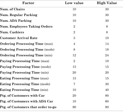
Each initial configuration set of factors is considered a data unit to be processed by the program. There are 18 total factors. Table 4.1.1 summarizes this information. The same table presents the values chosen to create the experimental plan. The values where chosen by selecting a high and low value for each factor such that the utilization of each process in the DES is within 50% to 95% in each configuration set. The processes in the ice cream store simulation are parking, customers order ice cream, the cashiers, and sit to eat.

Optimizing the design of the Ice-Cream Store involves testing all different configuration sets with the chosen values. Using the values presented in Table 4.1.1, there are 218_{different configuration sets to test, which results in running}

the simulation 262,144 times. The advantage of using a data-parallel implementation to run the DES is that each execution of the simulation can split into different processors and execute simultaneously. This reduces the execution time of the program to a fraction of the total.

[image:41.612.108.543.144.290.2]

(42)

A preliminary screening test indicates that it takes between 10 sec. and 40 sec., with some exceptions, to run each configuration set using the values defined in Table 4.1.1. The preliminary screening test consists of a 218-13

fractional factorial design with resolution III, running in one node of the parallel environment to sidestep the need of partitioning the data without yet having a data partitioning method implemented, and elude variances that small differences in the processors might add to the execution time measurements. A resolution III design can estimate the significance of the

Factor Low value High Value

Num. of Chairs 10 30

Num. Regular Parking 10 30

Num. ADA Parking 10 30

Num. Employees Taking Orders 2 8

Num. Cashiers 2 8

Customer Arrival Rate 3 10

Ordering Processing Time (max) 4 14

Ordering Processing Time (mode) 8 18

Ordering Processing Time (min) 12 24

Paying Processing Time (max) 2 10

Paying Processing Time (mode) 15 15

Paying Processing Time (min) 20 20

Eating Processing Time (max) 15 15

Eating Processing Time (mode) 7 30

Eating Processing Time (min) 10 40

Ptg. of Customers with Car 20 80

Ptg. of Customers with ADA Car 10 60

[image:42.612.96.520.128.514.2]

Ptg. of Customers that order to-go 80 80

Table 4.1.1- Variable factors considered for the data partition in the data

(43)

main effects, but may be confounded with two-level interaction. However, this design is sufficient for an initial screening.

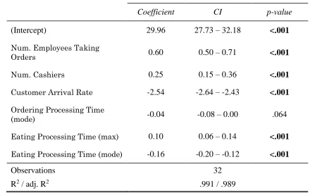
After fitting a main effects linear model to the sampling of the data obtained, the arrival rate factor is notably more significant in predicting the execution time of the simulation. Table 4.1.2 presents a summary of the model fit. The regression coefficient associated to arrival rate in the linear equation is -2.54 with a p-value of 2x10-16_{. The remaining factors have a regression}

coefficient within ±0.70 and p-values that range from 1x10-11_{to 6.41x10}-2_{. The}

p-value determines the significance of a factor. A p-value below the critical value means that the factor has a significant influence over the response. The critical value is set by the experiment. For this example, the critical value is set to be 0.05, which provides a 95% confidence on the significance of the factor. Other factors that can be considered significant from this analysis are num. of employees taking orders from customers, num. of cashiers, the mode component of the time to place a customer order, and the mode component of the eating time.

The significance of the factors can be explained by looking at some examples. First, if the arrival rate of customers into the system changes from one simulation to another then each simulation will process different amounts of events associated to each customer. If there are less customers coming into the system, there is a decrease in the number of events related to taking orders and making payments. Therefore, there are fewer instructions executed by the program.

(44)

Main Effects Linear Regression Model

Coefficient CI p-value

(Intercept) 29.96 27.73 – 32.18 <.001

Num. Employees Taking

Orders 0.60 0.50 – 0.71 <.001

Num. Cashiers 0.25 0.15 – 0.36 <.001

Customer Arrival Rate -2.54 -2.64 – -2.43 <.001

Ordering Processing Time

(mode) -0.04 -0.08 – 0.00 .064

Eating Processing Time (max) 0.10 0.06 – 0.14 <.001

Eating Processing Time (mode) -0.16 -0.20 – -0.12 <.001

Observations 32

R2 / adj. R2 .991 / .989

In addition to single factor effects, the compounded effects of factor interactions also affect the execution time of the simulation. A resolution III design, such as the one used to make the preliminary screening, cannot be used to determine the compounded effect of factor interactions. Hence, a new experimental plan was designed to gather sampling data from the execution of the program.

The new experimental design is a 218-9 _{two-level fractional factorial design}

[image:44.612.86.526.144.418.2]

consisting of a careful selection of 512 configuration sets of factors based on the high/low values presented in Table 4.1.1. The design has a resolution V, which states that a statistical analysis based on this design can estimate the independent effect that factors can have over the execution time of a simulation without confounding the effect of other factors and without confounding the

Table 4.1.2- Summary of the main effects linear regression model fit for

(45)

effect of two or three level interactions. It can also estimate the effect of two-level interactions without confounding the effect of other two two-level interactions.

In order to gather execution times to create a sampling of the data the program can only run in one node of the cluster. Again, to sidestep the need of partitioning the data without yet having a data partitioning method implemented and elude nuisance that small differences in the processors might add to the execution time measurements.

Based on the results from this experiment, Figure 4.1.2 shows interaction plots for the effect of two-level interactions on the execution time. The interaction plots highlight the significance of change in the execution time by changing one factor while given the value of another factor. For example, the average time between customer arrivals (arrival rate) and the number of employees taking order form the customers, as shown in Figure 4.1.2 (a). Decreasing the number of employees taking orders in a simulation with low arrival rate would not be as significant as it would be in a simulation with higher arrival rate. In the high arrival rate scenario, having more employees taking orders can reduce the number of customers waiting in queues, reducing the time associated to the logic of pushing and pulling elements from queues in the program. However, in a simulation with low arrival rate, there might not even be customers in a queue that could benefit from a large number of employees taking orders. This means that the magnitude of the effect in reducing the processing time is dependent on the value of the arrival. The same applies if comparing the relation between number of cashiers and the number of employees taking orders, as shown on Figure 4.1.2 (b). In this scenario, the processes are linked sequentially and one processes is performed after the other in the simulation logic; delays in the time taking orders affects the time paying. However, if the delay is in the cashiers then the other process is not affected.

(46)

example, in Figure 4.1.2 (a), the significance of change in the execution time by changing the number of employees while given the value of arrival rate can represent a difference of 15 to 20 sec. In Figure 4.1.2 (b), the difference in the execution time of changing the number of cashiers given the value of number of employees taking orders is less than 5 sec. Therefore, a predictive model must account only for significant interactions.

Using data sampling gathered from the previous experiment will provide the information necessary to create an accurate statistical model that can efficiently estimate main effects and two-level interactions.

(47)

The technique applied for variable selection is a stepwise regression with bi-directional elimination. The ‘stepAIC( )’ function from the MASS library in R [14] was used to automate the process. The final fit model possesses 16 main factors and 21 two-level interactions along with a coefficient of determination (R2₎_{of 0.98. The strong R}2_{value means there is a strong relation between}

factors and execution times. However, such a high number of variables in the model can suggest a problem of overfitting. It can affect the predictive quality of the model when exposed to other data samples.

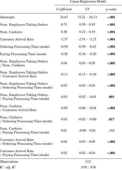
From the preliminary screening analysis, it was determined that not all factors are significant. Hence, another model was created to reduce the amount of factors while maintaining an acceptable quality in the model. The new model was created applying a Manual Backwards Elimination approach in R, as explained in Section 3.2.4. The final fit model created possesses 5 main factors and 9 two-level interactions, and a coefficient of determination R2 _{of 0.97. Table}

4.1.3 presents a summary this model.

(48)

Linear Regression Model

Coefficient CI p-value

(Intercept) 34.67 33.21 – 36.13 <.001

Num. Employees Taking Orders 0.75 0.59 – 0.92 <.001

Num. Cashiers 0.38 0.22 – 0.55 <.001

Customer Arrival Rate -2.37 -2.51 – -2.23 <.001

Ordering Processing Time (mode) -0.50 -0.58 – -0.43 <.001

Paying Processing Time (mode) -0.28 -0.36 – -0.20 <.001

Num. Employees Taking Orders

:: Num. Cashiers 0.04 0.03 – 0.05 <.001

:: Customer Arrival Rate -0.11 -0.13 – -0.10 <.001

:: Ordering Processing Time (mode) 0.03 0.02 – 0.03 <.001

:: Paying Processing Time (mode) -0.01 -0.02 – -0.01 .001

Num. Cashiers

:: Customer Arrival Rate -0.05 -0.06 – -0.04 <.001

Num. Cashiers

:: Ordering Processing Time (mode) -0.01 -0.02 – -0.00 .017

Num. Cashiers

:: Paying Processing Time (mode) 0.01 -0.00 – 0.01 .154

Customer Arrival Rate

:: Ordering Processing Time (mode) 0.04 0.03 – 0.05 <.001

Customer Arrival Rate

:: Paying Processing Time (mode) 0.03 0.02 – 0.04 <.001

Observations 512

[image:48.612.107.523.131.711.2]

R2 / adj. R2 .978 / .978

Table 4.1.3- Summary of the final model fit for the Ice-Cream Store

(49)

Having created a model, the parallel implementation was adapted to apply a data partitioning using the greedy algorithm. The idea is to sort the data units based on the estimated execution times, then pull out the first data unit in each step, and assign it to the subset with the smallest estimated processing time so far in the execution of the algorithm. A detailed explanation of greedy algorithm is presented in Chapter 2, Section 2.6.2.

A second example of the same program was adapted to apply the greedy algorithm based on the model presented in Table 4.1.2 – Only main effects model. The purpose is to compare the efficiency of the greedy algorithm under different sorting criteria and test the quality of the models created.

Given that the prescreening analysis determined that arrival rate has a notable significance compared to other factors, a third implementation of the program was adapted to use arrival rate as the only driving factor in the processes. This means the new model assumes that the expected execution time of the simulation is entirely dependent upon the arrival rate. In order to do that, the estimated execution time for the configuration sets with the low value for arrival rate was set at 15 sec. For the configuration sets with the high value for arrival rate, the estimated execution time was assigned to 35 sec. These values determined the results from the preliminary screening indicating a need between 10 sec. and 40 sec. to run each configuration set.

A fourth example of the same program was adapted to apply an equal sized data partition. This approach, instead of using the greedy algorithm, splits the 218_{data units in 16 batches of 13,107 runs each and 4 batches of 13,108 runs}

each (218_{/ 20) to be processed different nodes. The reason to choose the equal}

sized data partition method is to compare one of the most common methods currently used in data parallel implementations.

Those implementations were tested over a data set with 262,144 configuration sets. The data set was created as a 218 _{full factorial with the}

(50)

utilizing the computer resources and will run for less time than an equal data partitioning approach.

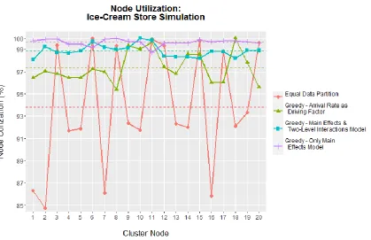
Figure 4.1.3 presents the overall utilization per node from running the programs in the cluster. The Node Utilization represents the percentage of the overall execution time of the program that a specific node was processing data. The Cluster Node enumerates from 1 to 20 and represents each of the 20 nodes in the Tropos Cluster in which the example application was run. The horizontal dotted lines represent the mean utilization per algorithm. The utilization is calculated as follows:

U = (execution time of the node)*100 / (largest execution time obtained)

In the figure, the greedy algorithm using the model in Table 4.1.3 – Main effects and two-level interactions model – performs as expected by utilizing the 20 nodes to almost 100% of its capacity through the entire program execution. The mean node utilization (𝜇) for this greedy algorithm is 98.86% with a

standard deviation(𝜎) of 0.54%. The greedy algorithm using the model in Table

4.1.2 – Only Main Effects model – performs just as well. The mean node utilization (𝜇) for this greedy algorithm is 99.63% with a standard deviation

(𝜎) of 0.29%. Such small variance, in both algorithms reflects a balanced

workload. There is no significant difference in the performance of each of the two greedy implementations. The model including only main effects performs just a as well as the model that also includes interactions.

(51)

In the same figure, the greedy algorithm that uses arrival rate as the only driving factor, has a mean node utilization (𝜇) of 97.37% and standard

deviation (𝜎) of 1.37%. The Equal Sized Data Partition approach has a mean

node utilization (𝜇) of 93.82% and standard deviation (𝜎) of 5.37%. Both

algorithms present an inefficient use of resources (higher variance in node utilization) compared to the other greedy approaches. The processing time associated to each percentage node utilization is presented later in Figure 4.1.5.

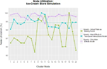
[image:51.612.98.517.265.536.2]

The next graph, Figure 4.1.4, presents the overall utilization per node excluding the equal data partitioning approach. The horizontal dotted lines represent the mean utilization per algorithm. The figure has better detail of the performance of the greedy approaches compared to each to other. Both greedy algorithms based on a model utilize the 20 nodes at 98% to 100% of its

(52)

capacity through the entire program execution. The greedy approach using arrival rate as a driving factor is clearly inefficient in terms of node utilization.

Figure 4.1.5 presents a graph with the total execution time per node for each implementation. The horizontal dotted lines represent the mean node execution time per implementation. As the figure shows, the mean time per node (𝜇) for all partitioning methods is around54.50 hrs. Nevertheless, for the

greedy algorithms using predictive models, there is a small variance compared to the equal sized data partitioning method and greedy algorithm with arrival rate as the driving factor.

The standard deviation (𝜎) of the total execution time per node for the

[image:52.612.94.512.140.408.2]

greedy algorithm using the model in Table 4.1.3 – Main effects and two-level interactions model – is 0.30 hrs. and the times range in the 95% confidence interval [54.48, 54.71]. For the greedy algorithm using the model in Table 4.1.2

Figure 4.1.4- Node Utilization Excluding Equal Data Partitioning

(53)

– Only Main Effects model – the standard deviation (𝜎) is 0.16 hrs. and the

times range in the 95% confidence interval [54.54, 54.66]. These results show that a greedy algorithm, based on an efficient predictive model, can perform a balanced workload among the nodes.

On the other hand, the greedy algorithm with arrival rate as the driving factor has a standard deviation (𝜎) of 0.77 hrs. and values that range in the

95% confidence interval [54.62, 55.21]. The equal data partition has standard deviation (𝜎) of 3.12 hrs. and values that range in the 95% confidence interval

[53.25, 55.66]. These two approaches present larger variances in the execution time per node, showing an imbalance in the workload among the nodes.

[image:53.612.95.513.318.586.2]

Figure 4.1.6 presents a graph with the total execution time per node excluding the equal data partitioning approach. Again, the figure has better detail of the performance of the greedy approaches compared to each to other.

Figure 4.1.5- Simulation-run Execution Times per Node: Ice-cream Store

(54)

Both greedy algorithms based on a model present a balanced workload distribution, while the greedy approach using arrival rate as a driving factor is more inefficient.

Part of the benefit of applying the proposed data partitioning method is to gain performance in the overall execution of the data-parallel program. This gain in performance is attributed to the improvement in computational resource utilization. A data parallel program execution will not finish until the last node has finished executing all assigned tasks, and therefore a bad partition can easily lead to unbalanced workloads and performance issues.

[image:54.612.100.515.153.427.2]

In order to demonstrate the opportunity of performance improvement, Figure 4.1.7 presents a bar chart that compares the total execution time for every data partitioning approach. Based on the figure, the equal data partitioning implementation ran for 58.04 hrs. The greedy algorithm based on

Figure 4.1.6- Simulation-run Execution Times per Node Excluding Equal

(55)

the model in Table 4.1.3 – Main effects and two-level interactions model – ran for 55.22 hrs. This represents a 4.85% gain in time compared to the equal data partition. The greedy algorithm using the model in Table 4.1.2 – Only Main Effects model – ran for 54.80 hrs. This represents a 5.58% gain in time compared to the equal data partition. The model including only main effects is slightly more efficient. However, the total time difference between both algorithms is less than 30 min. This means that there is no significant difference using one model or the other one. Such improvement determines that both models are effective at predicting execution times.

In the same figure, the greedy algorithm using arrival rate as the only driving factor ran for 56.40 hrs. This represents a 2.83% gain in time compared to the equal data partition. A better partition than the equal sized approach means that arrival rate has a large influence over the execution time. However,

(56)

the improvement is low compared to the other greedy approaches. It can be concluded that arrival rate is not the only driving factor in the model. Therefore, this sorting criterion for the greedy algorithm is not the desired aspect to exploit the capacity of the method.

The proposed methodology requires an initial training period to create the model. This training period refers to experimental plan execution. In the current example, the training period to create a model with main effects and two level interactions was of 2.44 hours. The training period to create a model with only main effects was of 0.14 hrs. There is no training period in creating a model where arrival rate is assumed the only driving factor of the process. Figure 4.1.8 presents the total execution time added to the training period for each implementation. The gain in performance does not look as significant as it was before. However, the training is meant to be run only once to determine the relation of the variables to the execution time. With a model created for repetitive processes the same model can be reused even if the value