doi:10.1006/ecss.2000.0591, available online at http://www.idealibrary.com on
E
ff
ects of Catchment Activities on Macrofaunal
Assemblages in Tasmanian Estuaries
G. J. Edgar
a,cand N. S. Barrett
baSchool of Zoology, University of Tasmania, GPO Box 252-05, Hobart, Tasmania, 7001 Australia
bTasmanian Aquaculture and Fisheries Institute, University of Tasmania, Crayfish Point Laboratory, Taroona,
Tasmania, 7053 Australia
Received 23 August 1999 and accepted in revised form 12 January 2000
Silt loadings associated with human activities in catchments were inferred to have an extremely widespread effect on estuarine macrobenthos around Tasmania. Estuaries with human population densities exceeding 10 km2
in catchments consistently possessed muddy rather than sandy beds and shores, and were dominated by infauna rather than epifauna. Estuaries with human population densities below 1 km2
in catchments possessed sandy sediments and numerous epifaunal species. These effects were consistent within groups of estuaries possessing similar hydrology and geomorphol-ogy. Although faunal composition differed substantially between estuaries possessing low and high human population densities, the number of macrofaunal species was similar. Population effects therefore could neither be detected using species richness indices, nor by the ABC method. Faunal changes were most clearly detected using disturbance indices weighted by the sensitivity of individual species to human activity. Two such indices, which are based on abundance (DIn) and productivity (DIp) data, are suggested to provide useful local indicators of estuarine health.
2000 Academic Press
Keywords: benthos; catchment processes; estuaries; human impacts; macrofauna; siltation; stress; Tasmania
Introduction
Shipping access, availability of dependable fresh water, prevalence of fertile alluvial land, and produc-tivity of waters for fish and shellfish have led world-wide to the concentration of human activity on estuaries. Changes to estuarine ecosystems inevitably follow development as a consequence of factors such as port construction (Whitfield, 1986), channel dredging (van Dolah et al., 1984), introduction of exotic taxa (Carlton, 1989), damming of migration routes (Rosenberg et al., 1995), reduction in fresh-water flows (Schlacher & Wooldridge, 1996), siltation (Newcombe & Jensen, 1996), marine farm pollution (Ritzet al., 1989;DeFur & Rader, 1995), and by the direct removal of ecologically-important fish and invertebrate species. Estuaries also provide access to hinterland regions, and serve as conduits for sewage (Cloern, 1996) and fertiliser (Lavery et al., 1991), mine runoff (Winemillter & Morales, 1989), indus-trial waste (Saiz-Salinaset al., 1996) and heated water (Bamber & Spencer, 1984). The outcome of these activities is often eutrophication (Nixon, 1995;
McClelland et al., 1997; Valiela et al., 1997) and
macrophyte loss (Silberstein et al., 1986; Boynton
et al., 1996), with nearly all estuaries outside polar regions suffering substantial anthropogenic degradation.
While the effects of human activity on estuarine ecosystems have been studied on numerous occa-sions, most studies have been confined to individual estuaries. More general assessments of the relative intensity of different human impacts at regional, national or international scales have not often been attempted (but see De Jonge et al., 1994). Hence in North America, for example, the question of whether the introduction of exotic species has caused greater disruption to estuarine communities than vegetation clearance remains unanswered. Clearly, the answer in this case will vary greatly between estuaries; how-ever, information on net effects at regional scales is crucial when assessing research priorities. Funding on noticeable human impacts within a few badly-degraded urbanized estuaries may well have occurred at the expense of identifying more subtle impacts affecting estuarine processes throughout large regions. The aim of the present study was to identify impacts on macrofaunal communities of human activity that extended over a regional scale of ]1000 km around Tasmania.
cTel: +61 3 6226 7632; Fax: +61 3 6226 2745; E-mail: [email protected]
Methods
Samples of macrofauna retained on a 1 mm sieve were collected using 150 mm diameter corers in-serted to a depth of 100 mm at 55 sites in 48 estuaries distributed around Tasmania and associ-ated Bass Strait islands, as described in more detail in Edgar et al. (2000). Sites were selected haphaz-ardly from the universe of estuarine sites around the coast and encompassed a wide range of environ-mental conditions, with salinities varying from 0 to 53, tidal range varying from 0 to 2·3 m, and estuary catchment area varying from 6 to 13 100 km2. At each site, cores were collected using a spatially-nested sampling design based on (i) three random transect lines perpendicular to the shore ]100 m apart, (ii) three to five fixed tidal heights down each transect (high water mark, mid tide level, low water mark, 0·3 m below low water, 0·7 m below low water), and (iii) two random replicates ]1 m apart at each height down each transect.
In the laboratory, samples were sorted into size-classes using a nested series of sieves. The biomass of each animal >2 mm sieve size was directly determined or estimated from length data and length/weight re-gressions. The biomass of animals <2 mm sieve size was estimated using general data on the mean biomass of animals associated with each sieve, as described in Edgar (1990). Estimates of the daily productivity of benthic invertebrates were calculated using bio-mass estimates for each animal and the equation P=0·0049*B0·80T0·89, which relates daily macro-benthic productivity P (g d1) to ash-free dry weight B (g) and water temperature T (C) (Edgar, 1990). Data collected in replicate samples from each site were amalgamated in the present study, with the mean density value for each species at each site used in analyses (Edgaret al., 1999).
Biological relationships between sites were assessed using non-metric multidimensional scaling (MDS), as run by the PRIMER program (Carr, 1996). The similarity matrices used in MDS were calculated between paired sites using the Bray-Curtis similarity coefficient after double root transformation, as recom-mended by Faith et al. (1987) and Clarke (1993). The usefulness of the MDS display of relationships between sites is indicated by the stress statistic, which if <0·1 indicates that the depiction of relationships is good, and if >0·2 that the depiction is poor (Clarke, 1993).
The density of individual species at the different sites was related to human activity using Spearman rank correlation coefficients. Species with high corre-lation values were positively associated with human
activity while species with low values were negatively associated. Human activity was quantified using two indices, the human population density and percent cleared land in catchment. In order to weight these two indices for activity in the immediate vicinity of the estuary, data for each site were calculated as the mean of the value for the total catchment area and the value for the estuarine drainage area. The estuarine drain-age area was defined as that region draining directly into the estuary rather than into the major associated river. The latter, in turn, was defined as occurring upstream of the point on 1:100 000 topographic maps where river banks were shown as separate lines, where the 10 m contour line crossed the river flow line, or where probable obstructions to tidal flow such as gorges were shown on maps (see Edgar et al., 2000).
Data on human population density and percent cleared land in catchments were obtained by over-laying GIS maps of catchment areas on digital popu-lation census and land use data sets (see Edgaret al., 1999,2000), following methods more fully described by Graddon (1997). Data on catchment land use were obtained by categorization of satellite images of the Tasmanian mainland, but were not available for estuaries on Bass Strait islands. Data on total annual runoff into estuaries were obtained by calibrating a GIS rainfall prediction model based on flow data from 63 gauged rivers and 504 rainfall stations (Edgar et al., 2000), while salinity, tidal range and the silt/clay content of sediments associated with each site were recorded in the field. Salinity was measured at 0·1 m depth below the surface during low tide, tidal range was estimated as the distance between the high tide layer of deposited flotsam and maximum retreat of water on the day of sampling, and the silt/clay (<63m) particle fraction was determined for aggregated sediments collected in shallow subtidal (0·3–0·7 m) depths. The latter vari-able was assessed at only 39 of the 55 sites sampled for macrobenthos.
Spearman rank correlation coefficients (Rs) relating animal abundance and human activity for all inverte-brate species across the 55 sites were used to calculate an index of anthropogenic disturbance (DI) for each site:
DIn=Rsi*ni/N
eliminated much of the largely irrelevant information associated with each site that was caused by variation in natural environmental factors such as salinity and tidal range rather than human impact, as well as ‘ noise ’ contributed by species that occurred at a wide range of sites but were not greatly influenced by human activity. Such an index was considered a potentially useful tool when monitoring changes to impacted habitats over time, and for assessing the spatial scale of impacts.
Comparable disturbance indices were also calcu-lated using data on the estimated productivity and biomass of macrofauna at each site (DIp=Rs
i*pi/P
and DIb=Rs
i*bi/B, where pi and bi represent total
productivity and biomass of species i, and P and
B represent total productivity and biomass of all macrofauna at the site).
Assessment of DI in the present study was partly confounded by circularity of calculations, in that indices were calculated using information on re-lationships between species abundance and distur-bance to estuaries (population density), and then tested using aggregated site information against the same population density variable. Ideally, derivation and assessment data sets should have been indepen-dent because any variable will show a relatively high correlation with DI when used also to calculate the weightings for each species that form the basis ofDI. To assess the scale of this bias, weightings for species were calculated using a dummy variable composed to random numbers, and then the corre-lation coefficient between DI and the original dummy variable calculated. The Abundance/Biomass Comparison (ABC) method of Warwick (1986) was also applied to the macrofaunal data set to assess whether this procedure has value in identifying sites subjected to human disturbance. In this procedure, the cumulative abundance and biomass of species ranked in order to importance in a sample were graphically compared for samples collected at four sites in estuaries with highest and lowest population densities in catchments. Only samples collected at or below low water mark were used in this analysis. Samples from higher tidal levels were excluded because they tended to be influenced by terrestrial as well as estuarine processes (Edgar & Barrett, unpublished data). Patterns of variation in the fauna were highly consistent between 0·3 and 0·7 m depth at sites examined. The hypothesis tested using the ABC procedure was that anthropogenic impact causes elevated densities of small individuals, hence total abundance is dominated by relatively few species compared to biomass under disturbed conditions (Warwick et al., 1987).
Results
Relationships between species abundance and human activity
Macrofaunal relationships between sites are depicted using MDS in Figure 1. The plot shown is three-dimensional because the equivalent two-three-dimensional plot produced a relatively poor description of the data (stress=0·12 cf. 0·17). The bubble plot overlay of human population density in catchment indicates that faunal assemblages varied between sites in a pattern related to population density (Figure 1). This corre-spondence occurred almost exclusively along MDS axis 1. The site with negligible population density at the extreme right of axis 1 was the Wanderer Estuary, an aberrant location with extremely low faunal pro-ductivity and little similarity to any other site (Edgar
et al., 1999). Percentage cleared land in catchment and silt-clay content of sediments at the sample site showed relatively poor relationships with macrofaunal assemblages.
Relationships between densities of species at sites and the level of anthropogenic disturbance, as as-sessed using Spearman rank correlation coefficients that relate total animal abundance at each site with human population density and percent cleared land, are listed for abundant species inTable 1. Significance values have not been assigned to correlation coef-ficients because of uncertainty caused by the large number of species investigated during the study increasing the probability of Type I error, and the generally small number of sites at which each species was recorded affecting the probability of Type II error. A total of 157 of the 390 taxa collected were recorded at a single site only, with the great majority of these animals considered marine vagrants (Edgar et al., 1999).
Population density was generally more highly cor-related with species abundance than percent cleared land, and therefore appeared to be the better discrimi-nator of human impacts. Population density produced a highest correlation coefficient of 0·51 for Tellina deltoidalis and a minimum value of 0·45 for Limnoporeia kingi, compared to maximum and mini-mum values amongst all species of 0·37 and 0·29 using percent cleared land data.
–2 2 2
MDS1
MDS2
1 0
–1 1
0
–1
Silt/clay fraction
–2 2
2
MDS1
MDS3
1 0
–1 1
0
–1
Silt (%)
0.1
1.0
10
–2 2
2
MDS1
MDS2
1 0
–1 1
0
–1
Cleared land
–2 2
2
MDS1
MDS3
1 0
–1 1
0
–1
Clearance (%)
1 5 20
–2 2
2
MDS1
MDS2
1 0
–1 1
0
–1
Human population density
–2 2
2
MDS1
MDS3
1 0
–1 1
0
–1
Density (km–2)
2 20 200
80 0.2 0
mudflat dwelling species (e.g. the bivalve Notospisula trigonella—Rs=0·40 and the crabs Heloecius cordiformis—Rs=0·28 and Helograpsus haswellianus—
Rs=0·24). By contrast, the six widespread species showing strongest negative correlations with popu-lation density were epifaunal species. This included three species that generally associate with sandflats in
similar salinity and tidal height conditions to the mudflat species (Eubittium lawleyanum, Hydrococcus brazieri and Exosphaeroma sp.). Most additional species with strong negative correlations with popula-tion density that were not included inTable 1because of restricted distribution were also sandflat inhabitants (e.g. the bivalve Wallucina assimilis—Rs=0·32 and T 1. Spearman rank correlation coefficients (Rs) relating abundance at different sites of
widespread species (i.e. the 46 species present at 12 or more sites) with population density (Pop) and % cleared land (Clear). Infaunal or epifaunal habit of species is also shown
Species Habit Group PopRs ClearRs
Tellina deltoidalis Infaunal Bivalve 0·51 0·37
Magelonasp. Infaunal Polychaete 0·39 0·30
Lumbrinerissp. 1 Infaunal Polychaete 0·39 0·35
Macrophthalmus latifrons Infaunal Crab 0·36 0·24
Nephtys australiensis Infaunal Polychaete 0·32 0·15
Callianassa arenosa Infaunal Shrimp 0·30 0·17
Nassarius burchardi Epifaunal Gastropod 0·26 0·15
Neanthes vaalii Infaunal Polychaete 0·24 0·26
Paragrapsus gaimardii Epifaunal Crab 0·22 0·19
Gammaropsissp. 1 Epifaunal Amphipod 0·21 0·01
Actaecia bipleura Epifaunal Isopod 0·19 0·27
Phyllodocesp. Epifaunal Polychaete 0·19 0·35
Limnoporeia yarrague Epifaunal Amphipod 0·18 0·22
Australonereis ehlersi Infaunal Polychaete 0·13 0·02 Dimorphostylis colefaxi Epifaunal Cumacean 0·09 0·04
Heteromastussp. Infaunal Polychaete 0·08 0·11
Mictyris platycheles Infaunal Crab 0·07 0·14
Exoediceroides ?maculosus Infaunal Amphipod 0·07 0
Nassarius pauperatus Epifaunal Gastropod 0·07 0·08
Mysella donaciformis Infaunal Bivalve 0·07 0·10
Paracorophium cf excavatum Infaunal Amphipod 0·06 0·20
Macrobrachiumsp. Epifaunal Shrimp 0·06 0·09
Pseudolana concinna Epifaunal Isopod 0·01 0·17
Xenostrobus inconstans Epifaunal Bivalve 0·04 0·02
Paracalliope australis Epifaunal Amphipod 0·05 0·17
Nemertean sp. 1 Infaunal Nemertean 0·06 0·05
Melitasp. Epifaunal Amphipod 0·07 0·20
Arthritica semen Infaunal Bivalve 0·11 0·01
Euzonussp. Infaunal Polychaete 0·11 0·05
Katelysia scalarina Infaunal Bivalve 0·11 0·03
Capitellasp. 2 Infaunal Polychaete 0·12 0
Tatea rufilabrus Epifaunal Gastropod 0·12 0·02
Leitoscoloplos normalis Infaunal Polychaete 0·12 0·15
Boccardiellasp. Infaunal Polychaete 0·13 0·09
Salinator fragilis Epifaunal Gastropod 0·14 0·12
Simplisetia aequisetis Infaunal Polychaete 0·15 0·25
Perinereis vallata Infaunal Polychaete 0·19 0·04
Chironomid spp. Epifaunal Insect 0·20 0·01
Zeacumantus diemenensis Epifaunal Gastropod 0·21 0·09
?Mysellasp. Infaunal Bivalve 0·24 0·10
Ascorhis victoriae Epifaunal Gastropod 0·27 0·23
Exosphaeromasp. Epifaunal Isopod 0·28 0·22
Hydrococcus brazieri Epifaunal Gastropod 0·28 0
Amarinus lacustris Epifaunal Crab 0·35 0·21
Eubittium lawleyanum Epifaunal Gastropod 0·38 0·29
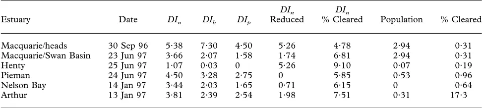
T2. Disturbance index values calculated using abundance (DIn), biomass (DIb) and productivity (DIp) data.DInwas also calculated using a reduced 30 species data set and using percent cleared land rather than human population density as the initial correlate. DIindices have been rescaled for comparisons in the range from 0 to 10 (where 0 indicates the site examined during the study with lowestDIand 10 the site with highestDI). Human population density and percent cleared land in catchment are also shown. Land clearance data were not available for seven estuaries on Bass Strait islands
Estuary Date DIn DIb DIp
DIn Reduced
DIn
% Cleared Population % Cleared
Sea Elephant 24 Feb 97 1·09 5·90 0·39 2·09 9·38 0·23 —
Yellow Rock 23 Feb 97 0·85 0 0·78 2·12 10·00 1·20 —
North East Inlet 8 May 97 2·41 5·34 1·34 2·64 4·50 0·12 —
Patriarch Inlet 9 May 97 2·26 5·82 1·88 1·72 4·24 0·06 —
Cameron Inlet 9 May 97 2·43 2·26 1·33 1·95 4·97 0·12 —
Modder 12 May 97 4·03 4·22 2·64 1·77 6·69 0 —
Rices 6 May 97 0 3·90 0·19 1·23 6·48 0 —
Welcome Inlet 21 Feb 97 0·01 2·64 2·01 2·01 4·23 0·57 22·0
Mosquito Inlet 22 Feb 97 3·11 5·78 1·23 2·52 2·86 0 1·43
East Inlet 15 Jan 97 2·78 7·80 2·23 2·55 2·69 7·61 49·2
Black/Dip 14 Jan 97 7·44 7·42 5·71 7·06 3·26 1·78 33·2
Detention 13 Jan 97 5·69 6·88 4·54 9·15 2·26 3·86 33·3
Cam 26 Sep 96 5·89 8·28 5·36 8·08 5·49 74·4 53·8
Blythe 16 Jan 97 6·02 9·21 7·63 8·99 4·72 25·7 28·2
Leven 25 Sep 96 7·14 5·62 3·36 9·95 1·24 71·6 45·6
Leven 17 May 97 7·37 3·91 3·84 9·39 1·44 71·6 45·6
Don 24 Sep 96 5·84 10·00 7·46 8·73 4·79 152·0 69·8
Port Sorell 17 Jan 97 6·23 0·69 3·14 8·77 1·97 11·9 31·2
Tamar/Low Head 16 Dec 96 6·14 5·55 4·83 8·17 3·05 39·8 36·00
Tamar/Paper Beach 17 Dec 96 9·15 7·08 10·00 9·91 0 39·8 36·00
Tamar/Paper Beach 17 Jun 97 10·00 5·70 9·86 10·00 0·13 39·8 36·00
Pipers 20 Nov 96 5·53 7·00 4·55 7·67 2·85 3·21 28·7
Tomahawk 22 Nov 96 4·30 7·14 3·09 7·40 5·25 0·63 52·5
Boobyalla 19 Nov 96 4·81 7·29 5·14 2·27 5·59 1·16 41·1
Little Musselroe Bay 14 Nov 96 1·26 4·05 0·33 1·12 3·12 0·39 72·7
Ansons Bay 12 Nov 96 4·93 6·52 3·28 4·34 4·40 2·82 8·21
Big Lagoon 13 Nov 96 2·46 5·95 1·64 2·06 8·86 0·14 1·28
Georges Bay 11 Nov 96 6·40 3·92 6·83 9·64 3·17 17·7 15·6
Hendersons Lagoon 13 Nov 96 3·14 6·01 4·87 6·81 6·06 1·04 25·7
Bryans Lagoon 13 May 97 1·36 2·04 0·79 2·10 9·48 0 0
Great Swanport 23 Dec 96 2·62 5·44 2·24 2·87 7·39 0·43 22·8
Lisdillon 17 Sep 96 2·68 0 4·14 2·41 7·31 3·66 42·9
Prosser 16 Sep 96 5·17 6·41 6·13 5·65 6·06 10·3 17·8
Earlham Lagoon 20 Aug 96 1·06 2·37 2·90 1·05 6·13 0·42 28·2
Pittwater 23 Oct 96 3·57 2·93 4·17 4·42 2·78 26·5 55·8
Derwent/Cornelian Bay 24 Apr 96 6·97 9·06 7·23 8·35 5·22 164·0 30·3
Derwent/Cornelian Bay 13 Feb 97 7·20 8·64 7·38 8·33 4·18 164·0 30·3
Derwent/Bridgewater 21 Oct 96 7·18 3·87 6·22 2·17 6·31 164·0 30·3
Derwent/Claremont 21 Oct 96 5·58 6·21 4·63 5·45 6·46 164·0 30·3
Browns 2 Jul 96 6·16 9·04 7·90 9·32 2·98 279·0 21·0
Huon/Eggs and Bacon 6 Nov 96 7·33 5·14 3·69 8·39 4·90 7·92 12·2
Huon/Brabazon 5 Nov 96 6·37 5·46 5·35 9·04 3·55 7·92 12·2
Huon/Cradoc 31 Oct 96 5·74 5·76 4·68 7·79 6·82 7·92 12·2
Huon/Cradoc 16 May 97 5·82 7·03 5·27 5·76 6·75 7·92 12·2
Hastings 9 Jan 97 5·66 6·61 4·78 9·02 5·64 0·95 0·57
Southport Lagoon 19 Jun 97 0·05 2·82 0·15 1·58 5·06 0 0
Cloudy Bay/southwest 18 May 97 1·22 2·07 1·85 2·52 6·17 0·32 10·7
Cloudy Bay/northeast 24 May 97 0·84 4·68 1·92 2·36 5·22 0·32 10·7
Cockle Creek 7 Jan 97 7·40 6·60 3·39 7·53 2·38 1·73 0
New River Lagoon 18 Feb 97 2·42 0·51 0·93 2·08 8·88 0 0
Bathurst Harbour 19 Feb 97 3·48 8·61 2·72 7·33 8·21 0·03 0
Payne Bay 19 Feb 97 0·72 1·93 1·86 2·06 5·24 0 0
the gastropods Diala suturalis—Rs=0·25 and
Haminoea maugensis—Rs=0·24).
Calculation of the disturbance index DIn for each site using Spearman rank correlation coefficients and abundance data indicated a wide range of values between sites. The site with the highest DI, and therefore the one most dominated by species typical of disturbed (i.e. heavily populated) conditions, was Paper Beach (Tamar Estuary) while Rices River was found to be the least disturbed.DInvalues for all sites sampled are listed inTable 2.
DInappears useful as an environmental indicator of anthropogenic disturbance of sites. It retains a high correlation with population density (Rs=0·74) and, to a lesser extent, with percent cleared land (Rs=0·55), but was not strongly correlated with the major physi-cal variable salinity (Rs=0·31). In addition, bubble plots overlayingDInvalues on MDS results showed a very good separation of sites (Figure 2), particularly for the plot of MDS axis 1vsaxis 3.DIntherefore has a high degree of faunal consistency and discriminates well between sites.
Disturbance indices based on reduced species data
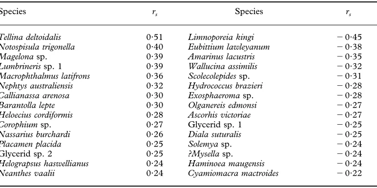
[image:7.595.47.536.98.207.2]In order to determine whether calculations of DIn were dominated by a limited number of influential species, this index was recalculated using data from the 15 species most highly positively and negatively correlated with human population density, as listed in
Table 3.
Correlation of DI values with human population density for sites calculated using the reduced species data set was similar to that for the full data set (Rs=0·73 cf. 0·74), hence little information had been lost. The bubble plots ofDI overlaying MDS results were also similar to plots obtained using all species (Figure 2).
Disturbance indices based on biomass and productivity data
DIwas also calculated using data on the total biomass (DIb) and estimated productivity (DIp) of species at each site rather than total numbers (DIn). The bubble plot overlays on MDS results (Figure 3) indicated that sites separated less strongly on the basis ofDIbthan on DIp or DIn. Relatively few sites possessed high DIp values (Table 2).
DIn and DIp both showed very little change over time, with DIp marginally more stable (see Table 2, where DI values for sites sampled on two occasions are shown). By contrast, DIb fluctuated considerably between sampling occasions, depending partly on the occasional collection of very large individuals. After DI was rescaled to range between 0 and 10, the average standard deviation at sites between times was 0·84 forDIbcompared with 0·25 and 0·24 forDInand DIprespectively.
DIpwas the best performing of all indices examined in terms of retaining its correlation with human popu-lation density (Rs=0·78, Table 4), while the corre-lation of DIb was relatively poor (Rs=0·40). DIpalso maintained a better correlation with the other distur-bance variable, percent cleared land, thanDInand was less influenced by the major physical variables salinity, tidal range and total annual runoff (Table 4). DIp maintained a high correlation with the silt/clay frac-tion of sediments, tidal range and total annual runoff. This, given the high correlation of population density itself with these variables, was expected. DIn, DIb and DIp were all moderately negatively correlated (0·49<Rs<0·28) with the density of animals at sites but were not greatly affected by the total biomass, total estimated productivity or total number of species.
Assessment of DI using species weightings calcu-lated for a dummy variable composed of random T2. (Continued)
Estuary Date DIn DIb DIp
DIn
Reduced
DIn
% Cleared Population % Cleared
Macquarie/heads 30 Sep 96 5·38 7·30 4·50 5·26 4·78 2·94 0·31
Macquarie/Swan Basin 23 Jun 97 3·66 2·07 1·58 1·74 6·81 2·94 0·31
Henty 25 Jun 97 1·07 0·03 0 5·26 9·10 0·07 0·19
Pieman 24 Jun 97 4·50 3·28 2·75 0 5·85 0·53 0·96
Nelson Bay 14 Jan 97 3·44 2·03 1·65 0·71 6·15 0 0·64
numbers, and then back correlated against DI, pro-duced a mean correlation coefficient of 0·49 for 50 dummy variables. This value was slightly higher than the correlation coefficient relating percent cleared land in catchment with theDInvalues calculated using that variable (=0·44, Table 4) and the correlation coefficient for DIb and population density (=0·40,
Table 4).DIcalculated using percent cleared land and DIb therefore both possessed negligible relationship with the biota.
By contrast, comparable correlation coefficients based on human population density data were very high for both DIn (Rs=0·74) and DIp(Rs=0·78). In terms of the proportion of total variance explained (R2), statistical bias assessed using dummy variables explained 24% (=0·492), leaving 31% (=0·742– 0·492) and 37% (=0·782–0·492) of the remaining
76% attributable to population density for DIn and DIp, respectively. After correction for circularity in calculations, the correlation coefficients between DI and human population density therefore remained high at 0·64 (=√(0·31/0·76)) and 0·70 (=√(0·37/ 0·76)) forDInandDIp, respectively.
Effects of estuary type
Because DI values and human population density were both highly correlated with other environmental variables, the possibility that the strong relationship between DI and population density was driven primarily by covariation with environmental factors rather than a direct relationship was examined by partitioning estuaries on the basis of geomorphologi-cal and hydrologigeomorphologi-cal type. Tasmanian estuaries were
–2 2
2
MDS1
MDS2
1 0
–1 1
0
–1
Reduced data set
–2 2
2
MDS1
MDS2
1 0
–1 1
0
–1
–2 2
2
MDS1
MDS2
1 0
–1 1
0
–1
Full data set
–2 2
2
MDS1
MDS3
1 0
–1 1
0
–1 DI
0.1
–0.1
–0.3 0.3
subdivided in an associated study (Edgaret al., 2000) into nine groups on the basis of biologically-important environmental characteristics (viz., presence of a seaward barrier, tidal range, salinity, estuary size and river runoff), with six of these estuary groups in-vestigated for macrofauna at more than three sites. Relationships between DI and human population density within these six estuary categories (barred low-salinity estuary, open polyhaline estuary, marine inlet, mesotidal river estuary, microtidal drowned river valley and open microtidal river estuary) were investigated using Analysis of Covariance (ANCOVA). Results based onDI as dependent vari-able, population density as independent variable (log x+0·1), and estuary type as grouping variable are presented inTable 5.
[image:9.595.98.484.106.299.2]None of the three DI indices showed a significant interaction between estuary type and log population density (analysis with interaction in Table 5), hence the slopes of the regression equations in different estuary types were similar and the interaction variable was removed from the second analysis. DIn and DIp both showed extremely strong relationships with population density after the effects of estuary were taken into account (analysis without interaction in
Table 5, P<0·001); however, DIb possessed no significant relationship with population density but a significant relationship with estuary type. The over-all significant relationship betweenDIband population density resulted from different estuary types possess-ing differing mean levels of DIb, and population density also differing significantly between the estuary types.
When comparable ANCOVAs were conducted using four other important environmental variables (tidal range, log total annual runoff, salinity and log silt/clay content of sediments) in place of human population density, no significant (=0·05) inter-actions were detected, hence slopes were also con-sidered homogenous in these ANCOVAs. Salinity and log total annual runoffwere found to vary significantly withDIonce the effects of different estuary types were taken into account (Table 6), although significant variation inDIoccurred between estuaries of different types.DInvaried significantly with tidal range within different estuary groups, whileDInandDIpalso varied with the percentage silt/clay content of sediments.
Relationships betweenDIn, human population den-sity in catchment, silt/clay content of sediments and estuary groups are shown as scatterplots in Figure 4. These relationships were non-linear, with negligible change in both DI and the silt/clay content of sedi-ments occurring for sites with population densities between 0 and 1 km2, rapid increases in dependent
variables occurring when densities were between 1 and 10 km2, and then little difference between sites
in catchments with densities >10 km2.
Abundance/biomass comparisons
Results ofWarwick’s (1986)ABC procedure for sites in estuaries with highest human population densities and sites lacking population within catchments are shown inFigure 5. Biomass curves lacked any consist-ent pattern in relation to abundance curves, rather than showing greater elevation at undisturbed sites, as T 3. Spearman rank correlation coefficients (Rs) relating human population density in
catchments with total abundance of animals for 15 species showing highest and lowest correlations
Species rs Species rs
Tellina deltoidalis 0·51 Limnoporeia kingi 0·45
Notospisula trigonella 0·40 Eubittium lawleyanum 0·38
Magelonasp. 0·39 Amarinus lacustris 0·35
Lumbrinerissp. 1 0·39 Wallucina assimilis 0·32
Macrophthalmus latifrons 0·36 Scolecolepidessp. 0·31 Nephtys australiensis 0·32 Hydrococcus brazieri 0·28
Callianassa arenosa 0·30 Exosphaeromasp. 0·28
Barantolla lepte 0·30 Olganereis edmonsi 0·27
Heloecius cordiformis 0·28 Ascorhis victoriae 0·27
Corophiumsp. 0·27 Glycerid sp. 1 0·25
Nassarius burchardi 0·26 Diala suturalis 0·25
Placamen placida 0·25 Solemyasp. 0·24
Glycerid sp. 2 0·25 ?Mysellasp. 0·24
Helograpsus haswellianus 0·24 Haminoea maugensis 0·24
would be expected if anthropogenic impact caused high densities of small species. The only noticeable trend in the complete data set, which includes sites not shown in Figure 5, related to the salinity of sites. Marine sites (e.g. Kelly Basin) were often dominated in terms of biomass by a few relatively large bivalves, while freshwater-influenced sites were generally in-habited by dense populations of small amphipods and hydrobiid gastropods.
Discussion
Biological indicators of human disturbance
The two anthropogenic disturbance indices proposed in this study,DInandDIp, appear to be sensitive
bio-logical indicators of human impacts within Tasmanian estuaries. Both indices were highly correlated with human population density within the catchment area, discriminated between sites with different faunal characteristics (Figure 2), and showed negligible change between different seasons. While these indices should prove useful for monitoring biological changes in Tasmanian estuaries over time, they have restricted geographic applicability because of their basis on correlation coefficients for individual species.
The index based on faunal abundance, DIn, has a single major advantage over the index based on faunal productivity, DIn, in that it is relatively simple to measure and comprehend. The advantage ofDIpover DInis that it is more biologically meaningful because DIpis not heavily biased by either large- or small-sized
–2 2
2
MDS1
MDS2
1 0
–1 1
0
–1
Productivity
–2 2
2
MDS1
MDS3
1 0
–1 1
0
–1
–2 2
2
MDS1
MDS2
1 0
–1 1
0
–1
Biomass
–2 2
2
MDS1
MDS3
1 0
–1 1
0
–1 DIb
0.1
–0.1
–0.2 0.2
DIp
0.2
0
–0.2 0.4
species (Edgar, 1990;Edgar & Shaw, 1995;Warwick & Clarke, 1993). Also, the productivity of a species is approximately proportional to total food consump-tion, total respiration and total reproductive output of that species, and so provides a relative index of its trophic importance (Edgar, 1993). By contrast, indi-ces which relate the abundance of a species to others have much less biological meaning because they can be influenced by one or two species of small size that contribute relatively little to the functioning of the community. Small species tend to be far more abundant in samples than large species.
An additional advantage ofDIpoverDInwas that it showed a higher correlation with percent cleared land, and so possibly responded to a wider range of human impacts (Table 4). DIp was also less strongly corre-lated with natural environmental variables (salinity,
tidal range, total annual runoff) and the total animal density of samples (rs=0·38 cf. 0·49).
The extent to which DIn and DIp are affected by natural physical factors and total sample size needs to be clarified in future studies. This is best done by manipulation of the level of anthropogenic impact independently of changes in physical factors. Such studies should also examine whether the biological indicators are affected by a large or narrow range of anthropogenic impacts, including siltation, nutrifi-cation, reduced oxygen concentrations and heavy metal concentrations.
Widespread human impacts in estuaries are likely to prove difficult to detect using methods other than disturbance indices, given that human impacts are often less obvious than pronounced relationships with natural environmental variables such as salinity (see T 4. Spearman rank correlation coefficients relating disturbance indices calculated using
abundance (DIn), biomass (DIb) and productivity (DIp) data, human population density and
en-vironmental variables. In addition to the full data set,DInwas calculated using a reduced 30 species
data set and using percent cleared land rather than human population density as the initial correlate
Variable DIn DIb DIp
DIn
Reduced
DIn
% Cleared Population
Population density 0·74 0·40 0·78 0·73 0·41 1·00
% Cleared land 0·37 0·28 0·46 0·43 0·44 0·67
Salinity 0·30 0·13 0·26 0·11 0·31 0·21
Tidal range 0·50 0·38 0·47 0·59 0·61 0·57
Latitude 0·18 0·02 0·24 0·20 0·17 0·16
Total annual runoff 0·52 0·12 0·47 0·35 0·10 0·49
% Silt/clay 0·59 0·29 0·60 0·45 0·18 0·65
Species number 0·10 0·15 0·02 0·13 0·36 0·11
Faunal density 0·49 0·28 0·38 0·55 0·53 0·26
Faunal biomass 0·04 0·09 0·05 0·12 0·40 0·14
Faunal productivity 0·08 0·15 0·11 0·04 0·28 0·12
T5. Results of Analyses of Covariance investigating the relationship betweenDIcalculated using abundance, biomass and productivity data and log-transformed human population density in catchments associated with estuaries grouped into six geomorphological and hydrological types
Effect DF
Abundance (DIn) Biomass (DIb) ProductivityDIp)
MS F P MS F P MS F P
Analysis with interaction
Estuary 5 8·854 5·026 0·001 11·293 2·782 0·030 2·553 1·619 0·177
Population 1 14·149 8·032 0·007 4·747 1·169 0·286 26·291 16·668 <0·001 Populationestuary 5 4·005 2·273 0·065 4·872 1·200 0·326 1·056 0·669 0·649
Error 41 1·762 4·059 1·577
Analysis without interaction
Estuary 5 5·803 2·894 0·024 19·259 4·644 0·002 3·400 2·236 0·067
Population 1 53·615 26·735 <0·001 3·508 0·846 0·363 71·345 46·919 <0·001
Edgar et al., 2000). Species richness provided a poor indication of human disturbance in Tasmanian estu-aries, largely because mudflats and sandflats con-tained faunas of similar species richness, as evident in the low correlation between population density and species number (Table 4). The Abundance/Biomass Comparison method for detecting human impacts (Warwick, 1986) also lacked usefulness because many of the infaunal mudflat species associated with high human population densities possessed relatively large body size and biomass (e.g.Tellina deltoidalis). Dauer
et al. (1993) have described similar problems in using the ABC method to detect stressed estuarine communities.
Furthermore, multivariate methods that incorpor-ate environmental variables into a predictive model based on undisturbed habitats, and then assess the difference between observed and predicted assem-blages (e.g.Mosset al., 1987), are also unsuitable for identifying impacted sites if sediment characteristics are included in the model. Such models will always predict a mudflat fauna for site with muddy sediments when sediment characteristics are incorporated as a habitat factor into the model.
Anthropogenic impacts on biota in Tasmanian estuaries
Macrofaunal species living in the upper and middle reaches of Tasmanian estuaries are adapted to a physical environment that undergoes rapid and
ex-treme fluctuations in salinity, temperature, water flow and turbidity. Most estuarine species also appear to be resilient to the effects of human disturbance. None of the major community metrics examined (species richness, faunal density, faunal biomass, faunal pro-ductivity) were found to be highly correlated with human population density or percent cleared land in catchments (Table 4).
Nevertheless, variation between estuaries in the disturbance indicesDInandDIprevealed clear diff er-ences between faunal assemblages in estuaries with different levels of human population density. Increas-ing population density was associated with increasIncreas-ing silt/clay content of sediments and with a reduction in number of epifaunal compared to infaunal species. These changes occurred consistently at relatively low human population densities, with virtually no overlap in DI or silt/clay content of sediments between estu-aries with <1 inhabitants km2 and estuaries with
>10 inhabitants km2.
Tasmania is unusual in a global sense in retaining a large number of estuaries with <1 inhabitants km2. If similar relationships with population density also apply in other regions, then biological communities in most temperature estuaries worldwide should be con-sidered to have already undergone major shifts as a result of human activity. Comparable studies con-ducted in most countries would possibly show little anthropogenic effect because of a lack of ‘ pristine ’ reference sites.
T6. Results of ANCOVAs relatingDIcalculated using abundance, biomass and productivity data to environmental variables (tidal range, log total annual runoff, salinity and log %silt/clay content of sediments) for estuaries grouped into six geomorphological and hydrological types
Effect DF
Abundance (DIn) Biomass (DIb) Productivity (DIp)
MS F P MS F P MS F P
Tidal range
Estuary type 5 21·19 7·629 <0·001 23 5·447 0·001 17·16 5·585 <0·001
Tide 1 18·09 6·512 0·014 0·014 0·003 0·954 0 0 0·99
Error 46 2·778 4·224 3·072
Total annual runoff
Estuary type 5 13·55 4·342 0·003 34·05 8·541 <0·001 15·06 5·032 0·001 Total annual runoff 1 2·322 0·744 0·393 10·95 2·747 0·104 3·646 1·218 0·275
Error 46 3·121 3·986 2·992
Salinity
Estuary type 5 21·34 6·796 <0·001 32·72 7·761 <0·001 19·75 6·46 <0·001
Salinity 1 1·438 0·458 0·502 0·362 0·086 0·771 0·661 0·216 0·644
Error 46 3·14 4·216 3·057
%silt/clay
Estuary type 5 17·88 11·03 <0·001 15 3·453 0·014 14·21 8·274 <0·001
Silt/clay 1 7·552 4·66 0·039 3·28 0·755 0·392 12·79 7·451 0·011
The correlations between human population den-sity, silt/clay fraction of sediments and faunal compos-ition may be due to direct dependence between these factors, or to indirect associations arising from shared relationships with other factors. Given the large number of studies that identify direct causal
relation-ships between human activities in catchments and increased sediment loads (e.g. Campbell & Doeg, 1989), the most likely hypothesis relating these factors is that anthropogenic activity in catchments and around estuary margins causes large inputs of fine suspended sediments that are transported to and
0
1000 100
Population density (km–2)
Sediment <63
µ
m (%)
10
1
0.1
0 0.1 1 10 100
–0.3
100 0.4
Sediment <63 µm (%)
Disturbance index
0.2
0.1
–0.1
0 0.1 1 10
1000 Population density (km–2)
Disturbance index
0 0.1 1 10 100
0.3
0.0
–0.2 –0.3 0.4
0.2
0.1
–0.1 0.3
0.0
–0.2
1 2 3 4 5 6 7 8 9 Estuary
group
deposited in the lower reaches of estuaries. These fine deposits coat the estuarine bed and eventually convert sandflats into mudflats, which attract infaunal species (such as Tellina deltoidalis and Magelona sp.) and displace epifauna (such as Eubittium lawleyanum and
Zeacumantus diemenensis).
An alternative hypothesis is that human settlement, with resulting high population densities, preferentially occurs in estuaries with muddy rather than sandy sediments, perhaps because of richer soils for
agricul-ture in the hinterland. While this hypothesis cannot be discounted outright, it is less likely than the previous hypothesis given the interspersion of estuaries with high and low human population densities studied around the state, and the extremely consistent rela-tionships between human population density, silt-clay content of sediments and DIn.
More importantly, results of the ANCOVAs indi-cated that DInand DIpboth increase with increasing human population density and silt/clay content of
100 Species rank Cumulative percentage 0 80 60 40 20
5 10 15
Browns Abundance Biomass 0 40 100 Species rank Cumulative percentage 80 60 40 20 35 Rices Abundance Biomass 0 10 100 Cumulative percentage 80 60 40 20 5 Don Abundance Biomass 0 15 100 Cumulative percentage 80 60 40 20 5 10 Bryans Lagoon Abundance Biomass 0 20 100 Cumulative percentage 80 60 40 20
5 10 15
Bridgewater Abundance Biomass 0 15 100 Cumulative percentage 80 60 40 20 5 10
New River Lagoon
Abundance Biomass 0 35 100 Cumulative percentage 80 60 40 20
5 10 15
Cornelian Bay Abundance Biomass 0 35 100 Cumulative percentage 80 60 40 20
5 10 15
Kelly Basin Abundance Biomass 30 25 20 15 10 5 Densely-populated Uninhabited 30 25 20 30 25 20
sediments within estuaries of similar geomorphologi-cal and hydrologigeomorphologi-cal type. Anecdotal information also consistently indicates that as human population den-sity increases within catchments the foreshores of associated estuaries change from sandflat to mudflat. For example, Cornelian Bay in the lower Derwent estuary possessed a sandy beach untilc. 1940, but the shore has since degraded and now includes large quantities of silt and clay (Sustainable Development Advisory Council, 1996).
While siltation is clearly an important factor associated with human impacts within estuaries, other factors also probably contributed to faunal differences between estuaries with low and high human popu-lation densities. This is indicated by the substantially lower correlation coefficient between DI and silt/clay content compared with DI and population density (Table 4), and the poor correspondence between silt/clay content and faunal assemblage type (Figure 1). Amongst the most probable contributing factors associated with human impacts are nutrification, eutrophication, seagrass loss and discharge of urban and industrial waste. Manipulative experimental work is required to distinguish between the influences of these and other potentially-important factors.
Acknowledgements
Amongst the many people who made the project possible, we would particularly like to thank Dave Graddon for undertaking the GIS work. The project was supported by funding from Ocean Rescue 2000 (Environment Australia) and an ARC Research Fellowship.
References
Bamber, R. N. & Spencer, J. F. 1984 The benthos of a coastal power station thermal discharge canal. Journal of the Marine Biological Association of the United Kingdom64,603–623. Boynton, W. R., Hagy, J. D., Murray, L., Stokes, C. & Kemp, C.
1996 A comparative analysis of eutrophication patterns in a temperature coastal lagoon.Estuaries19,408–421.
Campbell, I. C. & Doeg, T. J. 1989 Impact of timber harvesting and production on streams: a review.Australian Journal of Marine and Freshwater Research40,519–539.
Carlton, J. T. 1989 Man’s role in changing the face of the ocean: biological invasions and implications for conservation of near-shore environment.Conservation Biology3,265–273.
Carr, M. R. 1996 PRIMER User Manual. Plymouth Routines in Multivariate Ecological Research. Plymouth Marine Laboratory, Plymouth, UK.
Clarke, K. R. 1993 Non-parametric multivariate analyses of changes in community structure.Australian Journal of Ecology18, 117–143.
Cloern, J. E. 1996 Phytoplankton bloom dynamics in coastal ecosystems: a review with some general lessons from sustained investigation of San Francisco Bay, California. Reviews of Geophysics34,191–202.
Dauer, D. M., Luckenbach, M. W. & Rodi, A. J. 1993 Abundance biomass comparison (ABC method): effects of an estuarine gradient, anoxic/hypoxic events and contaminated sediments. Marine Biology116,507–518.
De Jonge, V. N., Boynton, W. D., D’Elia, C. F., Elmgren, R. & Welsh, R. L. 1994 Responses to developments in eutrophication in four different North Atlantic estuarine systems. InChanges in Fluxes in Estuaries: Implications from Science to Management(Dyer, K. R. & Orth, R. J., eds). Olsen & Olsen, Fredensborg, Denmark. pp. 179–196.
DeFur, P. L. & Rader, D. N. 1995 Aquaculture in estuaries: Feast or famine?Estuaries18,2–9.
Edgar, G. J. 1990 The use of the size-structure of benthic macro-faunal communities to estimate macro-faunal biomass and secondary production. Journal of Experimental Marine Biology and Ecology 137,195–214.
Edgar, G. J. 1993 Measurement of the carrying capacity of benthic habitats using a metabolic-rate based index.Oecologia95,115– 121.
Edgar, G. J. & Shaw, C. 1995 The production and trophic ecology of shallow-water fish assemblages in southern Australia. III. General relationships between sediments, seagrasses, inverte-brates and fishes. Journal of Experimental Marine Biology and Ecology194,107–131.
Edgar, G. J., Barrett, N. S. & Last, P. R. 1999 The distribution of macroinvertebrates and fishes in Tasmanian estuaries.Journal of Biogeography26,1169–1190.
Edgar, G. J., Barrett, N. S., Graddon, D. J. & Last, P. R. 2000 The conservation significance of estuaries: a classification of Tasmanian estuaries using ecological, physical and demographic attributes as a case study.Biological Conservation92,383–397. Faith, D. P., Minchin, P. R. & Belbin, L. 1987 Compositional
dissimilarity as a robust measure of ecological distance.Vegetatio 69,57–68.
Graddon, D. J. 1997 Characteristics of Tasmanian estuaries and catchments: physical attributes, population, and land use. Master of Environmental Studies thesis, University of Tasmania, Hobart. Lavery, P. S., Lukatelich, R. J. & McComb, A. J. 1991 Changes in the biomass and species composition of macroalgae in a eutrophic estuary.Estuarine and Coastal Shelf Science33,1–22.
McClelland, J. W., Valiela, I. & Michener, R. H. 1997 Nitrogen-stable isotope signatures in estuarine food webs: A record of increasing urbanization in coastal wetlands.Limnology and Ocean-ography42,930–937.
Moss, D., Furse, M. T., Wright, J. F. & Armitrage, P. D. 1987 The prediction of the macro-invertebrate fauna of unpolluted running-water sites in Great Britain using environmental data. Freshwater Biology17,41–52.
Newcombe, C. P. & Jensen, J. O. T. 1996 Channel suspended sediment and fisheries: A synthesis for quantitative assessment of risk and impact.North American Journal of Fisheries Management 16,693–727.
Nixon, S. W. 1995 Coastal marine eutrophication: a definition, social causes, and future consequences.Ophelia41,199–219. Ritz, D. A., Lewis, M. E. & Shen, M. 1989 Response to organic
enrichment of infaunal macrobenthic communities under salmonid seacages.Marine Biology103,211–214.
Rosenberg, D. M., Bodaly, R. A. & Usher, P. J. 1995 Environ-mental and social impacts of large scale hydro-electric develop-ment: who is listening?Global Environmental Change5,127–148. Saiz-Salinas, J. I., Ruiz, J. M. & Frances-Zubillaga, G. 1996 Heavy metal levels in intertidal sediments and biota from the Bidasoa Estuary.Marine Pollution Bulletin32,69–71.
Schlacher, T. A. & Wooldridge, T. H. 1996 Ecological responses to reductions in freshwater supply and quality in South Africa’s estuaries: lessons for management and conservation.Journal of Coastal Conservation2,115–130.
Sustainable Development Advisory Council 1996 State of the Environment, Tasmania, Volume 1—Conditions and Trends. Department of Environment & Land Management, Hobart. Valiela, I., Kremer, J., Lajtha, K., Geist, M., Seely, B., Brawley, J.
& Sham, C. H. 1997 Nitrogen loading from coastal watersheds to receiving estuaries: New method and application. Ecological Applications7,358–380.
van Dolah, R. F., Calder, D. R. & Knott, D. M. 1984 Effects of dredging and open water disposal on benthic macroinvertebrates in a South Carolina estuary.Estuaries7,28–37.
Warwick, R. M. 1986 A new method for detecting pollution effects on marine macrobenthic communities.Marine Biology92,
557–562.
Warwick, R. M., Pearson, T. H. & Ruswahyuni 1987 Detection of pollution effects on marine macrobenthos: further evaluation of the species abundance/biomass method. Marine Biology 95,
193–200.
Warwick, R. M. & Clarke, K. R. 1993 Comparing the severity of disturbance: a meta-analysis of marine macrobenthos community data.Marine Ecology Progress Series92,221–231.
Whitfield, A. K. 1986 Fish community structure response to major habitat changes within the littoral zone of an estuarine coastal lake.Environmental Biology of Fishes17,41–51.