ENERGY SAVING SCHEDULING FOR EMBEDDED
REAL-TIME LINUX APPLICATIONS
Claudio Scordino
and
Giuseppe Lipari
Scuola Superiore Sant’Anna
Viale Rinaldo Piaggio, 34 - 56025 Pontedera - Pisa, Italy
{
[email protected],[email protected]
}
Abstract
The problem of reducing energy consumption is becoming very important in the design of embedded real-time systems. Many of these systems, in fact, are powered by rechargeable batteries, and the goal is to extend, as much as it is possible, the autonomy of the system. To reduce energy consumption, one possible approach is to selectively slow down the processor frequency.
In this paper we propose a modification of the Linux kernel to schedule aperiodic tasks in a soft real-time environment. The proposed solution consists in a new scheduling strategy based on the Resource Reservation Framework [9], which introduces very little modification to the Linux API. Our scheduler is based on Algorithm GRUB (Greedy Reclamation of Unused Bandwidth), presented by Baruah and Lipari [5].
After presenting the algorithm, we describe its implementation on a Intrinsyc CerfCube 250, which uses a Intel PXA250 processor. We show with an example of multimedia application that, by using our approach, we save up to 38% of energy with respect to an unmodified Linux.
1
Introduction
Although there is a mathematical theory to exactly formalize the behaviour of a real-time system, some-times the design of these systems is still made in a rough way. Some designers consider that a fast enough system is always able to respond in a satis-factory way, and do not consider other factors (like size, cost, or energy consumption) that are decisive in the embedded systems sector.
The problem of reducing energy consumption is be-coming very important in the design and implemen-tation of embedded real-time systems. Many of these systems are powered by rechargeable batteries, and the goal is to extend as much as it is possible the autonomy of the system. A similar problem is being addressed in normal workstation PCs. As processors become more and more powerful, their energy con-sumption increases correspondingly, and it becomes a problem to dissipate the heat produced by the pro-cessor.
To reduce energy consumption, one possible ap-proach is to selectively slow down the processor fre-quency. By reducing the frequency, it is also possible to reduce the voltage at which the processor is
func-tioning, so reducing the power consumption. For ex-ample, if the processor has little to do for a certain interval of time, by reducing the frequency we slow down the processor speed but we can still complete all activities in time.
However, by reducing the frequency and the proces-sor speed, we increase the load of the system. In particular, a certain task will take more time to be executed. In real-time systems, this means that some important task may miss its deadline. Therefore, it is important to identify the conditions under which we can safely slow down the processor without missing any deadline.
In this paper we propose a modification of the Linux scheduler that is able to change the processor fre-quency reducing the energy consumption, guaran-teeing at the same time that no task will miss its deadline. The proposed solution consist in a new scheduling strategy based on the Resource Reserva-tion Framework , which introduces very little modifi-cation to the Linux API. Basically, a new scheduler, called SCHED CBS is available to the user of an ap-plication. In this way, it is possible to apply the same technique also to legacy Linux code.
After presenting the algorithm, we describe its imple-mentation on a Intrinsyc CerfCube 250, which con-sists of a Intel PXA250 processor with 32Mb of Flash ROM and 64 Mb of SDRAM. We configured the sys-tem to support three different frequencies, 100Mhz, 200Mhz and 400 Mhz. The modified OS is Linux 2.4.18. We show an experiment in which we compare an unmodified version of Linux with our modified version. In the experiment, we run a multimedia ap-plication where tasks are dynamically activated and suspended with a highly variable load. We show that by using our approach, we save up to 38% of energy with respect to an unmodified Linux.
This work has been done in the context of the OCERA project (IST-35102), which is financially supported by the European Commission.
2
Related Work
It’s not easy to compare our work with other exist-ing solutions. This is essentially due to two elements of difference: the kind of real-time system, and the kind of experimental tests.
We work in an aperiodic environment, so the prob-lem is not so trivial as in a periodic context, where if a task stops, then it will not execute until the next period (as in [7]). In our system a task could activate at any time. This assumption reduces the set of time points in which we can safely reduce the frequency clock.
Moreover, our results are not based upon some simu-lation (as in other works): we actually implemented our scheduling policy in Linux (creating a soft real-time system) and we actually measured the amount of energy used by the system.
3
Algorithm GRUB
We chose to implement the Greedy Reclamation of Unused Bandwidth algorithm ([5]), which is an im-provement of theConstant Bandwidth Server ([2]). GRUB is an algorithm belonging to the class of aperi-odic servers with dynamic priorities. This technique consists in creating an entity, referred as server, that manages a set of tasks. However, a limit of some ape-riodic servers with dynamic priorities is that they rely on the knowledge of execution times of served aperiodic tasks. In some cases, though, the execu-tion time of a task is unknown, or extremely variable from an instance to another (consider, for example, a MPEG player). In these cases, the use of a hard real-time system to manage this kind of applications would be unsuitable for two reasons:
• First, the worst case execution time (WCET) of the job could be much higher than its av-erage execution time. Since the guarantees for hard real-time tasks are given on the basis of the WCET (and not on the basis of the average execution time), this kind of applications could cause an enormous waste of resources. In fact, the system is sized according to the WCET of each real-time task, and this leads to a very partial utilisation of the performance that it could offer.
• Second, it’s hard to provide an exact evalu-ation of the WCET. The fact that the real-time guarantees depend on the evaluation of the WCET of each job, makes the hard real-time system weak respect to some mistake in this evaluation. If a job doesn’t respect the evaluated execution time, another task could miss its deadline.
GRUB is not affected by this problem because it doesn’t rely on an evaluation of the WCET. It guar-antees temporal isolation among tasks: as a conse-quence, a task can’t affect the performance of an-other task.
In our model, each server is characterised by two pa-rameters, (Ui,Pi), whereUi is the server bandwidth
(or fraction of the processor utilisation) andPiis the
period. Algorithm GRUB provides an abstraction of “slower processor”: the task served by a server Si
with bandwidthUi executes as it were executing on
a dedicated slower processor with a minimum speed equal toUi times the speed of the real processor.
The periodPi represents thegranularityof the time
from the point of view of the server. The smallerPi,
the closer is the virtual time to the real-time. Each task τi executing on server Si generates a
sequence of jobs J1
i, Ji2, Ji3, . . . , where J j
i
be-comes ready for execution (arrives) at timeaji (aji ≤ aji+1∀i, j), and requires a computation time of cji. We assume that, inside each server, these jobs are executed in FIFO order, i.e. Jij has to finish before Jij+1 can start executing.
We make the following requirements of our schedul-ing discipline:
• The arrival times of the jobs (theaji’s) are not a priori known, but are only revealed on line during system execution. Hence, our schedul-ing strategy cannot require knowledge of future arrival times.
• The exact execution requirements cji are also not known beforehand: they can only be deter-mined by actually executingJij to completion. (Nor do we require an a priori upper bound
(a “worst-case execution time”) on the value ofcji.)
• We are interested in integrating our schedul-ing methodology with traditional real-time scheduling — in particular, we wish to design a scheduler that is a minor variant of the clas-sical Earliest Deadline First scheduling algo-rithm (EDF) [1].
In this paper, we will consider a system comprised ofnserversS1, S2, . . . , Sn, with each serverSi
char-acterized by the parametersUi and Pi as described
above. Furthermore, we restrict our attention to sys-tems where all of these servers execute on a single shared processor (without loss of generality, this pro-cessor is assumed to have unit processing capacity) — we therefore require that the sum of the proces-sor shares of all the servers sum to no more than one; i.e., n X i=1 Ui ! ≤1.
The following theorem formally states the per-formance guarantee that can be made by Algo-rithm GRUB vis a vis the behaviour of each server when executing on a dedicated processor. For a proof of this theorem, see [5].
Theorem 1 Suppose that jobJij would begin execu-tion at time-instant Aji, if all jobs of server Si were
executed on a dedicated processor of capacity Ui. In
such a dedicated processor,Jijwould complete at time instantFij def= Aji+ (eji/Ui), whereeji denotes the
ex-ecution requirement ofJij. IfJij completes execution by time-instantfij when our global scheduler is used, then it is guaranteed that
fij≤Aji + & (eji/Ui) Pi ' ·Pi . (1)
For the previous inequality, it follows that fk i <
Fk
i +Pi. This is what we intend when we say that
Piis the temporal granularity of the server: by using
algorithm GRUB, every job finishes at mostPi time
units later than the completion time on a dedicated slower processor.
Several other server-based global schedulers (e.g., CBS [2]), can offer performance guarantees some-what similar to the one made by Algorithm GRUB. However, Algorithm GRUB has an added feature that is not to be found in many of the other sched-ulers — an ability to reclaim unused processor ca-pacity (“bandwidth”) that is not used because some of the servers may have no outstanding jobs awaiting execution.
Now, we describe the algorithm.
Algorithm Variables. For each server Si in the
system, Algorithm GRUB maintains two variables: adeadline Di and avirtual time Vi.
• Intuitively, the value ofDi at each instant is a
measure of thepriority that Algorithm GRUB accords server Si at that instant —
Algo-rithm GRUB will essentially be performing earliest deadline first (EDF) scheduling based upon theseDi values.
• The value ofViat any time is a measure of how
much of serverSi’s “reserved” service has been
consumed by that time. Algorithm GRUB will attempt to update the value of Vi in such a
manner that,at each instant in time, serverSi
has received the same amount of service that it would have received by time Vi if executing on
a dedicated processor of capacity Ui.
Algorithm GRUB is responsible for updating the val-ues of these variables, and will make use of these variables in order to determine which job to execute at each instant in time.
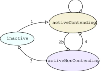
At any instant in time during run-time, each server Si is in one of three states: Inactive,Active Contend-ing, or Active Non Contending. The initial state of each server isInactive. Intuitively at time toa server
is in the Active Contendingstate if it has some jobs awaiting execution at that time; in the Active Non Contendingstate if it has completed all jobs that ar-rived prior toto, but in doing so has “used up” its
share of the processor until beyondto(i.e., its virtual
time is greater thanto); and in the Inactive state if
it has no jobs awaiting execution at time to, and it
hasnot used up its processor share beyondto.
At each instant in time, Algorithm GRUB chooses for execution some server that is in its Active Con-tending state (if there are no such servers, then the processor is idled). From among all the servers that are in their Active Contending state, Algo-rithm GRUB chooses for execution (the next job needing execution of) the serverSi, whose deadline
parameterDiis the smallest.
While (a job of) Si is executing, its virtual time
Vi increases (the exact rate of this increase will be
specified later); while Si is not executing Vi does
not change. If at any time this virtual time be-comes equal to the deadline (Vi == Di), then the
deadline parameter is incremented by Pi (Di ←
Di+Pi). Notice that this may causeSi to no longer
be the earliest-deadline active server, in which case it may surrender control of the processor to an earlier-deadline server.
State Transitions. Certain (external and inter-nal) events cause a server to change its state (see Figure 1). inactive activeContending activeNonContending 1 2a 2b 3 4
FIGURE 1: State transition diagram.
1. If serverSiis in theInactivestate and a jobJij
arrives (at time-instantaji), then the following code is executed
Vi←aji
Di←Vi+Pi
and server Si enters the Active Contending
state.
2. When a job Jij−1 of Si completes (notice that
Simust then be in itsActive Contendingstate),
the action taken depends upon whether the next jobJij ofSihas already arrived.
(a) If so, then the deadline parameter Di is
updated as follows:
Di←−Vi+Pi ;
the server remains in the Active Contend-ingstate.
(b) If there is no job ofSiawaiting execution,
then server Si changes state, and enters
theActive Non Contendingstate.
3. For serverSito be in theActive Non Contend-ing state at any instant t, it is required that Vi > t. If this is not so, (either immediately
upon transiting into this state, or because time has elapsed but Vi does not change for servers
in the Active Non Contendingstate), then the server enters theInactivestate.
4. If a new jobJij arrives while serverSi is in the Active Non Contendingstate, then the deadline parameterDi is updated as follows:
Di ←−Vi+Pi ,
and serverSi returns to theActive Contending
state.
5. There is one additional possible state change — if the processor is ever idle, thenall servers in the system return to theirInactivestate. Algorithm GRUB mantains a global variable total system utilisationthat, at every instant, is equal to
U =
n
X
i=1,Si6=Inactive
Ui
wherenis the number of servers in the system. This variable is initialised to 0 and it is updated ev-ery time a server enters in or exits from stateInactive. In particular, whenSi exits from stateInactiveU is
increased ofUi, whereas whenSienters stateInactive
it is decreased ofUi.
The rule for updating the virtual time of every server is as follows: d dtVi = U Ui ifSi is executing 0 otherwise (2)
Let us make an example to understand the way the algorithm works. Consider a serverS1 with
band-widthU1= 0.25 and periodP1= 20msec that serves
a MPEG player that needs to visualise 25 frames per second. If the system is fully utilised (i.e. the total system bandwidthU is equal to 1), then Equa-tion 2 tells us that the virtual time is increased at a rate of 1/0.25 = 4. By looking at the algorithm rules, we see that the server executes approximately P1/4 = 5msec every periodP1.
In general, the bandwidthU1can be computed using
some rule of thumb, or by performing a careful anal-ysis of the application code. For our purpouses, in this example we assume that in the worst case 5msec are enough to visualise a frame in most cases. However, suppose that at some point the total sys-tem utilisation U is equal to 0.75. Then, server S1
can execute more than 5msec every period, because we can reclaim the spare bandwidth. According to Equation 2, the virtual time is increased at a rate of 0.75/0.25 = 3. This means that our server will be able to execute forP1/3 = 6.66msec every period.
Thus, if our application sometime requires more than 5msec to display a frame, it can take advantage of the reclaimed bandwidth and still execute inside the period boundary. This property can help us in set-ting the server bandwidth U1 to a lower value. For
example we can decide to setU1 equal to the
aver-age bandwidth required by the application. Algo-rithm GRUB ensures that our application will take advantage of the spare bandwidth and execute more thanU1P1in most cases. This property of GRUB is
called “reclamation”, because we are giving the spare bandwidth to the needing servers.
3.1
Power-aware scheduling
We can use GRUB to decide when the frequency of the processor can be changed. As first step, let us assume that the processor speed can be varied con-tinuosly, from a maximum speed factor of 1 (i.e. the processor works at its maximum speed) to a mini-mum of 0 (i.e. processor is halted). As explained previously, GRUB maintains a global variableUthat is the sum of the bandwidths of all servers that are not in theInactive state. The key idea is that, if we set the speed factor of the processor to be equal to U, no server will miss its deadline.
In practice, if the processor is not fully utilised (U < 1) the exceeding bandwidth (1−U) can be used in two ways:
1. To execute the active servers for a longer time, so that they can execute faster and finish ear-lier. This is the “reclamation” property, and it is the original goal the GRUB algorithm was designed for.
2. To slow down the processor. Each active server will still execute for a longer time, but they will execute at a slower speed. The net effect is that their performance is not degraded.
Let us make an example to understand how it works. Suppose that we have a server S1 with bandwidth
U1 = 0.2 and period P1 = 10msec. If U = 1, it
means that the system is fully utilised, i.e. there are many servers in the system that are not in the
Inactive state, and the sum of their bandwidth is equal to 1. Under these conditions, our server S1
will be allowed an execution of 2msec every period P1= 10msec. If the system utilisationU goes down
to 0.5 (for example because some server has no job to execute and is in theInactivestate), then our server S1is allowed to execute for (U1/U)P1= 4msec units
of time. If we slow down the processor speed to a factor of 50%, the server still executes the same amount of code as in the first case, because it ex-ecutes twice as much (4msec instead of 2msec) but at half the speed. Therefore, the performance of the tasks served by serverS1 does not change.
Of course, no existing processor can vary its speed with continuity. So, we set some “thresholds” on the values of the total system bandwidth. If the sys-tem bandwidth goes below a certain threshold we can lower the processor frequency, and hence the proces-sor speed. The implementation details of the algo-rithm are explained in the following sections.
4
Implementation details
4.1
Generic Scheduling
Since we want to limit as much as it is possible the modifications to the standard Linux scheduler, we decided to apply a small patch (called Generic Scheduler Patch) that exports the necessary kernel symbols. Then, we implemented our scheduler as a loadable kernel module.
Our scheduler needs to “intercept” the job arrival (i.e. tasks that are unblocked) and the job finishing (i.e. tasks that are blocked). Moreover, the scheduler must know when tasks are created and when tasks terminate.
Therefore, we decided to export an inter-face to the scheduler through the standard sched_setscheduler()system call, adding a new scheduling policy, calledSCHED_CBS, and extending the structuresched_param.
For this reason, the Generic Scheduler Patch exports the followinghooksthat can be used to intercept the interesting scheduling events:
block hook is invoked when a task is blocked, such that the scheduler understands that the cur-rent job has finished.
unblock hook is invoked when a task is unblocked, such that the scheduler is informed of the ar-rival of a new job.
fork hook is invoked when a new task is created by a fork() and a pointer to the task is passed as parameter.
cleanup hook is invoked when a task is termi-nated, such that the scheduler can free the in-ternal resources.
setsched hook is invoked when the system calls sched_setscheduler()orsched_setparam() are called by the user.
All the hooks, except setschedsched_hook have a parameter that is a pointer to the structure task_structof the corresponding task.
The patch inserts a new field called private_data in thetask_struct, of type void *. It is a pointer used by our scheduler to access the private real-time data of every task. In our case, it is a pointer to the server that handles the task. If necessary, the scheduler must set this field to the appropriate data structure during the fork_hook. When the module is removed, it must ensure that all tasks have their private_dataset to NULL.
Our dynamically loadable scheduler modifies the task priority, raising the selected task to the max-imum priority, and then calls the standard Linux
scheduler. Based on the information received by the hooks, our scheduler selects which task has to be exe-cuted and sets its policy toSCHED_FIFOorSCHED_RR and thert_priorityto the maximum real-time pri-ority + 1. Then, it invokes the Linux scheduler. In practice, the Linux scheduler acts as a dispatcher for our scheduler. Thus, the modification to the stan-dard Linux scheduler are minimal. In particular, our implementation will take advantage of the more effi-cient scheduler that is being provided by Ingo Molnar for the next version of Linux.
Note that in this implementation, the scheduling al-gorithm does not assume any periodic behaviour of the task. As matter of fact, the scheduler only inter-cepts the blocking/unblocking events of a task, and it is the task’s responsibility to implement a periodic behaviour, if required. Thus, our scheduler is able to serve any kind of task, from non-periodic legacy Linux processes to periodic soft real-time tasks.
4.2
CPU clock frequency assignment
The hardware we used in our experiments is a In-trinsyc CerfCube 250, consisting of 32 MB Flash ROM, 64 MB SDRAM, and a Ethernet 10/100 Mbps. The processor is an Intel PXA250. It is a super-pipelined 32 bits RISC processor based on the Intel Xscale micro-architecture. This architecture permits a on-the-fly switch of the clock frequency and a so-phisticated power consumption management. In particular, the processor can be in one of the fol-lowing states:1. Turbo Mode: the processor core works at the peak frequency.
2. Run Mode: the processor core works at its “normal” frequency. In this mode, it is as-sumed that the processor frequently accesses external memory, so it is convenient for it to work at a frequency lower than the Turbo Mode frequency.
The register in which it is possible to select the clock frequency is called CCCR (Core Clock Con-figuration Register) and can be found at the address 0x41300000. The CCCR register manages the core clock frequency which the memory controller clock, the LCD clock and the DMA clock depend upon. In this register, the following parameters are specified:
- Frequency multiplier from the quartz frequency to the memory controller (L)
- Frequency multiplier from the memory fre-quency to the CPU frefre-quency in Run Mode (M)
- Frequency multiplier from the CPU frequency in Run Mode to the CPU frequency in Turbo Mode (N)
The value of L is chosen depending on the constraints of the external memory and of the LCD and it is usu-ally constant, while the values of M and N can change in order to change the speed of the processor. Value M is chosen based on the bus speed constraints and on the minimal performance requirements. Value N is based on the values of peak performance.
To modify the system clock frequency, register CCLKCFG can be used, that is register number 6 of the co-processor 14 (which is dedicated to power management at the lower level). It is a 32 bit register that is used to enter the Turbo Mode and the Fre-quency Change Sequence. Register CCLKCFG can only be modified through the following assembler in-structions.
• To read the value of the register and put it in R0, you must use
MCR p14, 0, R0, c6, c0, 0
• To copy the content of registerR0into register CCLKCFG, you must use
MRC p14, 0, R0, c6, c0, 0
To ensure that the Turbo bit does not change when we enter the Frequency Change Sequence, we must perform a read-modify-write sequence of assembler instructions.
As you can see, there is a great deal of flexibility in setting the clock frequencies. We had to choose how to implement our algorithm, which frequency to use as base frequencies, and so on. We decided to use only 3 levels for the processor clock frequency (100 MHz, 200 MHz, 400 MHz), whereas the mem-ory frequency does never change. By using these 3 levels, we are able to use the minimum possible fre-quency (100 Mhz) and the maximum one (400 Mhz). Therefore, we have two thresholds,Uth1 = 1/4 and
Uth2= 1/2.
One detail that must be taken into careful considera-tion is the overhead of changing frequency. Changing frequency is not “for free”, as the processor take some time (order of tens to hundreds of micro-seconds) to adjust to the new frequency. Althought this is not so high, it cannot be ignored. In particular we want to avoid limit situations in which the processor keep changing its frequency up and down, because this would completely trash the system.
When an increase of the total system bandwidth U goes over one of the thresholds, we immediately in-crease the processor frequency. Indeed, even if it could be a short transitory peak we cannot be sure and we do not want to risk a degradation of the tem performances. When a decrease of the total sys-tem bandwidth U goes below one of the threshold, instead, we do not change the frequency immediately. In fact, in case of a short temporary decrease of the bandwith, we could end up changing the frequency very often up and down. Therefore, when U goes below a threshold, we set a timer. If the timer ex-pires andU is still below the threshold we lower the frequency.
Now we compute the maximum overhead of the fre-quency switch. Let δbe the maximum time it takes to switch frequency and let ∆ be the timer expira-tion interval. We can have a maximum of 2 frequency switches every ∆, one to go down and another one to go up. Therefore, in the worst case this accounts for a bandwidth reduction of 2δ
∆.
In our implementation, the timeout duration is a customisable parameter of the algorithm, called PWR_TIMEOUTwhich specifies the timer’s duration in seconds.
Every threshold level is described by the following struct: struct pwr_level { int bandwidth; int run_mode; int turbo_mode; int selected;
struct t_data_struct pwr_timer; };
The first parameter (bandwidth) is the maximum bandwidth that this level can support (the band-width is expressed as an integer because we use a fixed point representation). The second and third pa-rameter are, respectively, the Run Mode multiplier (M) and the Turbo Mode multiplier (N). Variable selected is used to handle the timer. When the total system utilisation goes below bandwidth, we set the timerpwr_timerand the variableselected. IfU goes above the thresholdbandwidthbefore the timer expiration, selected is set to false, and the timer is canceled.
A global variable
struct pwr_level* current_pwr_level;
points to the current power level.
5
Experimental results
One may argue that varying the processor frequency only, without touching the peripherals frequencies
(like memory, for example) does not bring apprecia-ble advantages. We will show that this is not the case.
Our study is particularly focused on multimedia ap-plications. Therefore, we decided to evaluate the performance of our system using a multimedia ap-plication. However, our approach can be used for a large range of different applications, because it is completely transparent to the application character-istics.
Unfortunately, our system, the Intrinsyc CerfCube, does not present a video output. So, we decided to focus our attention to a audio decoder. We selected the decoder provided by the Xiph.Org Foundation that is a “non-profit organisation dedicated to pro-tecting the foundations of Internet multimedia from control by private interests”. Ogg Vorbis is a non-proprietary compressed audio format that provides high quality (from 8 to 48 bits, polyphonic) with fixed or variable bitrate that ranges from 16 to 128 Kbps per channel. It is in direct competition with MPEG-4 et similia.
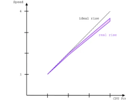
To execute the first test, we decompressed some au-dio stream at 44100 Hz and two channels, measuring the time necessary to decompress every stream under the different fixed clock frequencies.
From the obtained values, we extracted how much the speed of decompression is related to the speed of the CPU. The result is shown in Figure 2, where we show on the x-axis the speed of the processor, and on the y-axis the decompression speed. As you can see the relationship is almost linear. This justifies our as-sumption that by doubling the processor speed, the computation time of one task’s job halves. In the Figure we also show the 99% confidence interval.
Speed 100MHz 200MHz 400MHz CPU Frequency 1 4 ideal rise real rise
FIGURE 2: Decompression speed related to CPU speed (99% confidence interval).
Then, we evaluated the power consumed by our sys-tem under different conditions, with or without our algorithm. We measured the current entering into the CerfCube with a circuit powered separately by a 9 V battery that measures the current and sends it to a host computer via serial communication. The
circuit puts a very small resistor in series with the CerfCube and measures the voltage at the ends of the resistor.
By using our algorithm, we measured the temporal evolution of the current under different loads. In Figures 3, 4, 5, we show the temporal evolution of the input current when the total load is U = 0.25, U = 0.5 andU = 1 respectively. 120 125 130 135 140 145 0 2000 4000 6000 8000 10000 FIGURE 3: Temporal evolution of the cur-rent with system bandwidth U = 0.25
155 160 165 170 175 180 185 190 0 500 1000 1500 2000 2500 3000 3500 4000 4500 5000 FIGURE 4: Temporal evolution of the cur-rent with system bandwidth U = 0.5
216 218 220 222 224 226 228 0 500 1000 1500 2000 FIGURE 5: Temporal evolution of the cur-rent with system bandwidth U = 1
We computed the average values of the input current, reported in the table 1.
CPU clock Current frequency
100 MHz 446.0 mA 200 MHz 508.5 mA 400 MHz 579.9 mA
TABLE 1: Average values of the input cur-rent.
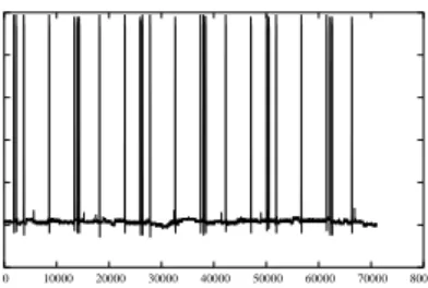
In Figure 6 we also report what happens with our al-gorithm when the total bandwidth goes from 0.1 to 1. As we said previouosly, the processor frequency is changed from 100 Mhz to 400 Mhz. The temporal evolution of the current is reported in Figure 6.
0 50 100 150 200 250 0 10000 20000 30000 40000 50000 60000 70000 80000 90000 FIGURE 6: Temporal evolution when the total bandwidth goes from 0.1 to 1
Our algorithm brings an advantage in two distinct situations.
Idle System. When the system is idle, we can lower the frequency to 100 Mhz. Without the frequency scaling mechanism, it is necessary to mantain the frequency to 400 Mhz all the time because we must guarantee maximum performance under peak load. The input current when the system is idle is shown in Figure 7. The average value of the input current is 250.5 mA. 0 2 4 6 8 10 12 14 16 18 20 0 5000 10000 15000 20000 25000 30000 35000 40000 FIGURE 7: An idle system with voltage scaling
If the voltage scaling algorithm is not activated and the system is idle, the input current is shown in Fig-ure 8. The average value of the input current is 406.8 mA. We can say that we save up to 38.4% of power in the average when the system is idle.
Non idle systems.When the system is not idle and the required total bandwidth is less than 1, it is pos-sible to find a clock frequency less than 400 Mhz that respects the performance of the applications. We run an application that decodes an audio stream using a bandwidth of 0.15. By using our voltage scaling algo-rithm we measured an average current of 343.6 mA, whereas without voltage scaling, the average current was 433.3 mA. Therefore, we saved up to 20.7%.
80 100 120 140 160 180 200 0 10000 20000 30000 40000 50000 60000 70000 80000 FIGURE 8: An idle system without voltage scaling
The most general case is when we have many applica-tions that activate and deactivate themselves many times. In that case, the load of the system is highly variable, and we can take fully advantage of the volt-age scaling algorithm.
We executed the audio decoder many times on dif-ferent audio streams. Every instance is assigned a different value of the bandwidth, so that the total bandwidth of the system goes up and down, as shown in Figure 9. We expect a similar behaviour in the temporal evolution of the input current.
U Linux 0.1 0.5 1 0.25 264.ogg 65.ogg 30.ogg 30.ogg 71.ogg 10sec t
FIGURE 9: Variation of the bandwidth during the test.
In Figure 10 we show the input current measured in the presence of the voltage scaling algorithm. You can verify that the temporal evolution is similar to the one of Figure 9. The average input current is 413.3 mA. 0 50 100 150 200 250 0 100000 200000 300000 400000 500000 600000 700000 FIGURE 10: Input current with voltage scaling 80 100 120 140 160 180 200 220 240 260 0 100000 200000 300000 400000 500000 600000 700000 FIGURE 11: Input current without voltage scaling
The input current measured with no voltage scaling is shown in Figure 11. The average input current is 461.2 mA. Therefore, we saved up to 10.4 %.
6
Conclusions
We modified the Linux OS in order to guarantee soft real-time tasks and at the same time reduce the power consumption. The resulting system is highly modular because is based on the Loadable Kernel Module feature of Linux. It currently supports In-tel PXA250 based architecture. We believe that it could be easily portable on different hardware archi-tectures. The code is distributed under the GPL and it can be dowloaded fromhttp://www.ocera.org.
References
[1] C.L. Liu, and J. W. Layland, January 1973, Scheduling Algorithms for Multiprogramming in a Hard-Real-Time Environment, Journal of
ACM, Vol. 20, No. 1, pp. 46-61.
[2] L.Abeni and G.Buttazzo, December 1998, Inte-grating Multimedia Applications in Hard Real-Time Systems, Proceedings of the IEEE Real-Time Systems Symposium, Madrid, Spain, pp. 4-13.
[3] Luca Abeni and Giuseppe Lipari, Decem-ber 2002, Implementing Resource Reservations in Linux, Real-Time Linux Workshop,
Boston (MA).
[4] Intel corporation, February 2002,Intel PXA250 and PXA210 Application Processors Devel-oper’s Manual,order number 278522-001. [5] Giuseppe Lipari and Sanjoy Baruah, June
2000, Greedy reclamation of unused bandwidth in constant-bandwidth servers, Proceedings of the EuroMicro Conference on
Real-Time Systems, Stockholm, Sweden, pp.
[6] Giuseppe Lipari and Sanjoy Baruah, May 2001, A hierarchical extension to the constant band-width server framework,Proceedings of the Real-Time Technology and Applications
Symposium, Taipei, Taiwan.
[7] H.Aydin, R.Melhem, D.Moss, P.Mejia-Alvarez, December 2001, Dynamic and Aggressive Scheduling Techniques for Power-Aware Real-Time Systems, Proceedings of Real-Time
System Symposium, London, UK,
pp.95-105.
[8] Ismael Ripoll, Pavel Pisa, Luca Abeni, Paolo
Gai, Agnes Lanusse, Sergio Saez, and Bruno Privat, 2002, WP1 - RTOS State of the Art Analysis: Deliverable D1.1 - RTOS Analysis,
Ocera(http://www.ocera.org).
[9] R. RajKumar, K. Juvva, A. Molano, and S. Oikawa, January 1998, Resource kernels: A resource-centric approach to real-time systems,
Proceedings of the SPIE/ACM Confer-ence on Multimedia Computing and
Net-working.
[10] Alessandro Rubini and Jonathan Corbet,Linux Device Drivers 2nd edition, O’REILLY.