University of Southampton Research Repository
ePrints Soton
Copyright © and Moral Rights for this thesis are retained by the author and/or other
copyright owners. A copy can be downloaded for personal non-commercial
research or study, without prior permission or charge. This thesis cannot be
reproduced or quoted extensively from without first obtaining permission in writing
from the copyright holder/s. The content must not be changed in any way or sold
commercially in any format or medium without the formal permission of the
copyright holders.
When referring to this work, full bibliographic details including the author, title,
awarding institution and date of the thesis must be given e.g.
AUTHOR (year of submission) "Full thesis title", University of Southampton, name
of the University School or Department, PhD Thesis, pagination
Perceptron-Like Large Margin Classifiers
by
Petroula Tsampouka
A thesis submitted in partial fulfillment of the requirements for the degree of Doctor of Philosophy
in the
Faculty of Engineering, Science and Mathematics School of Electronics and Computer Science
ABSTRACT
FACULTY OF ENGINEERING, SCIENCE AND MATHEMATICS SCHOOL OF ELECTRONICS AND COMPUTER SCIENCE
Doctor of Philosophy
PERCEPTRON-LIKE LARGE MARGIN CLASSIFIERS
by Petroula Tsampouka
Acknowledgements iii
0 Introduction 1
0.1 Overview . . . 1
0.2 Contributions . . . 3
0.3 Publications . . . 4
0.4 Thesis Outline . . . 4
1 Kernel-Induced Feature Spaces 6 1.1 Data Representation . . . 6
1.2 Learning in the Feature Space . . . 7
1.3 Implicit Mapping via a Kernel. . . 8
1.4 Characterisation of Kernels . . . 10
1.5 Examples of Kernels . . . 15
2 Elements of Statistical Learning Theory 18 2.1 The General Inference Model . . . 18
2.2 Learning from Examples . . . 20
2.3 Minimising the Risk Functional . . . 21
2.4 Consistency of the Learning Process . . . 23
2.5 Empirical Processes . . . 28
2.6 The Key Theorem of Learning Theory . . . 30
2.7 Entropy and Other Related Concepts. . . 31
2.8 Bounds on the Rate of Convergence . . . 33
2.9 The VC Dimension . . . 38
2.10 The Structural Risk Minimisation Principle . . . 40
2.11 The ∆-Margin Hyperplane. . . 43
2.12 Concluding Remarks . . . 47
3 Support Vector Machines 49 3.1 The Motivation behind Support Vector Machines . . . 49
3.2 Separating Hyperplanes . . . 50
3.3 The Optimal Margin Hyperplane . . . 52
3.4 Soft Margin Hyperplanes . . . 57
3.5 Implementation Techniques . . . 60
4 Incremental Algorithms 64 4.1 Introduction. . . 64
4.2 The Augmented Space . . . 65
4.3 The Perceptron Algorithm . . . 66
4.4 The Second-Order Perceptron Algorithm. . . 67
4.5 The Perceptron Algorithm with Margin . . . 70
4.6 Relaxation Procedures . . . 71
4.7 The Approximate Large Margin Algorithm . . . 72
4.8 The Relaxed Online Maximum Margin Algorithm. . . 74
4.9 The Maximal Margin Perceptron . . . 76
5 Analysis of Perceptron-Like Large Margin Classifiers 82 5.1 Preliminaries . . . 82
5.2 Relating the Directional to the Geometric Margin. . . 83
5.3 Taxonomy of Perceptron-Like Large Margin Classifiers . . . 84
5.4 Stepwise Convergence . . . 86
5.5 Generic Perceptron-Like Algorithms with the Standard Margin Condition 88 5.6 The ALMA2 Algorithm . . . 91
5.7 The Constant Rate Approximate Maximum Margin Algorithm CRAMMAǫ 94 5.8 The Mistake-Controlled Rule Algorithm MICRAǫ,ζ . . . 100
5.9 Algorithms with Fixed Directional Margin Condition . . . 105
5.9.1 Generic Perceptron-Like Algorithms with Fixed Margin Condition 106 5.9.2 Algorithms with Constant Effective Learning Rate and Fixed Mar-gin Condition . . . 108
5.9.3 Mistake-Controlled Rule Algorithms with Fixed Margin Condition 111 5.9.4 Algorithmic Implementations . . . 112
6 Linearly Inseparable Feature Spaces 114 6.1 Introduction. . . 114
6.2 A Soft Margin Approach for Perceptron-Like Large Margin Classifiers . . 116
6.3 Generalising Novikoff’s Theorem to the Inseparable Case. . . 120
7 Implementation and Experiments 123 7.1 Comparative Study of PLAs. . . 123
7.1.1 Separable Data . . . 124
7.1.1.1 The Sonar Dataset. . . 124
7.1.1.2 The Artificial Dataset LS-10 . . . 130
7.1.1.3 The Dataset WBC−11 . . . 132
7.1.2 Inseparable Data . . . 135
7.1.2.1 The WBC Dataset . . . 135
7.1.2.2 The Votes Dataset . . . 138
7.2 A “Reduction” Procedure for PLAs. . . 140
7.3 Comparison of MICRA with SVMs . . . 141
7.4 An evaluation . . . 146
8 Conclusion 147
I would like to thank my supervisor Professor John Shawe-Taylor for his advice and support.
Introduction
0.1
Overview
Machine learning deals with the problem of learning dependencies from data. The machine (algorithm) is provided with a training set consisting of examples drawn in-dependently from the same distribution. We distinguish three main learning problems: the problems of classification (pattern recognition), regression and density estimation. In the classification task the examples are given in the form of instance-label pairs with the labels taking integer values which indicate which out of a certain number of classes the instances belong to. In the regression task each instance is accompanied by a real number related to it either through an unknown deterministic functional dependency or in the most general case through a conditional probability. Finally, in the density estimation task no additional information is provided to the machine other than the instances themselves. In the training process the machine tries to infer a functional relation mapping the input space of instances to the output space which is either the set of discrete values that the labels take (in the classification task) or the set of real numbers (in the regression task). In the density estimation task in which the machine is looking for the underlying distribution governing the data no such mapping exists. Any such function that the machine returns as an output is known as a hypothesis. In the present work we will only be concerned with the binary classification problem in which the labels can take only one out of two values.
The goal of the machine is to construct a hypothesis able to predict the labels of in-stances which did not participate in the training procedure. If we impose no restriction on the functions which the machine chooses its hypothesis from it might be that most of the instances of an independent set will be wrongly classified by the hypothesis pro-duced even though this hypothesis explains the training data satisfactorily. The above situation can be remedied if the richness of the function class employed by the machine is appropriately restricted. There are various classes of functions which the learning
algorithms draw their hypothesis from with the most prominent ones being the classes of linear functions, polynomials and radial basis functions.
By embedding the data in an appropriate feature space via a nonlinear mapping we can always use a machine employing the class of linear discriminants. The hyperplane generated by the machine which performs the separation of the training examples in the feature space corresponds to a nonlinear curve in the original space. In many learning algorithms the mapping can be efficiently performed by the use of kernels. Therefore, the treatment of classes which contain nonlinear functions can be considered a straight-forward extension of the linear case whenever the kernel trick is applicable.
A broad categorisation of the algorithms could be done according to the learning model that they follow. In the first category are those algorithms that follow the online model. According to the online model learning proceeds in trials and the instances become accessible one at a time. More specifically, in each trial the algorithm observes an instance and makes a guess of its binary label. Then, the true label of the instance is revealed and if there is a mismatch between the prediction and the actual label the algorithm incurs a mistake. The algorithm maintains in every trial a hypothesis defining the linear discriminant which is updated with every mistake. A natural extension of online learning is the incremental or sequential setting of learning in which the algorithm cycles repeatedly through the examples until no mistake occurs. The most prominent algorithm in this category is the Perceptron [47]. In the second category belong the algorithms which follow the batch learning model and which have access to all training instances prior to the running of the algorithm. Well-known examples of algorithms in the second category are the Support Vector Machines (SVMs) [9]. The SVMs solve an optimisation problem with a quadratic objective function and linear constraints. SVMs in contrast to Perceptrons minimise the norm of the weight vector defining the solution hyperplane. This is actually equivalent to maximising the minimum distance (margin) of the training instances from that hyperplane.
The algorithms that reach convergence find, in the linearly separable case, a hypothesis consistent with the training data. However, even such solutions may fail to classify correctly unseen (test) data. The ability of a hypothesis to classify correctly test data is known as the ability to generalise. The generalisation ability of a linear classifier is believed to be enhanced as the margin of the training instances from the hyperplane solution becomes larger. This favours considerably algorithms like SVMs which find solutions possessing large margin.
to any accuracy. Such algorithms include the Maximal Margin Perceptron [34], agg-ROMMA [38] and ALMAp [21]. In order to obtain solutions with margin their
misclas-sification condition (i.e. the condition that decides whether a mistake occurs) becomes stricter and is satisfied not only if the predicted label of the instance is wrong but also in the case of correct classification with a lower than the desirable value of the margin. Our work presented here follows the same line.
0.2
Contributions
Our main contributions are the following:
We developed Perceptron-like algorithms with margin in which the misclassification condition is modified to require a fixed value of the margin. These new algorithms are radically different from the previous approaches which implement a misclassification condition relaxing with time (i.e. with the number of mistakes). With the condition kept fixed two generic classes of algorithms emerged, the one leaving the length of the weight vector determining the hypothesis hyperplane free to grow indefinitely and the other keeping the weight vector normalised to a fixed length. The new algorithms converge to a solution with a fixed value of the margin in a finite number of steps and may be used as modules of more complex algorithmic constructions in order to approximately locate the optimal weight vector. Additionally, we introduced stepwise convergence, the ability of the algorithm to approach the optimum weight vector at each step, and making use of it we developed a unified approach towards proving convergence of Perceptron-like algorithms in a finite number of steps. This research led to [56].
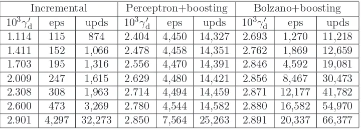
We also introduced the “effective” learning rate, the ratio of the learning rate to the length of the weight vector, and performed a classification of Perceptron-like algorithms into four broad categories according to whether the misclassification condition is fixed or relaxing with time and according to whether the effective learning rate is fixed or decreasing with time. The classification revealed that the Perceptron with margin and ALMA2belong to the same category whereas the algorithms with fixed margin condition
margin extension for Perceptron-like large margin classifiers was presented following the approach of [17] and was shown to correspond to a partial optimisation of an appropriate criterion. This research led to [57].
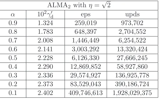
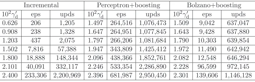
Finally, we constructed MICRAǫ,ζ an approximate maximum margin algorithm in which both the effective learning rate and the misclassification condition are entirely controlled by rules involving powers of the number of mistakes. Since the effective learning rate of MICRA decreases with the number of mistakes there is no condition on its initial value for convergence to occur. CRAMMA may be regarded as a limiting case of MICRA with the parameter ζ controlling the rate of decrease of the effective learning rate set to zero. We provided a theoretical analysis of MICRA and investigated the conditions under which MICRA converges asymptotically to the optimal solution with maximum margin. We also presented a variation of the standard sequential way of cycling through the data which leads to considerable improvement in running times. An extensive com-parative experimental investigation revealed that MICRA with ǫ≪1 andζ ≃1 is very competitive. This research led to [58].
0.3
Publications
This work has contributed to the following publications:
• Tsampouka, P., Shawe-Taylor, J.: Analysis of generic perceptron-like large margin classifiers. ECML 2005, LNAI3720 (2005) 750–758, Springer-Verlag
• Tsampouka, P., Shawe-Taylor, J.: Constant rate approximate maximum margin algorithms. ECML 2006, LNAI 4212 (2006) 437–448, Springer-Verlag
• Tsampouka, P., Shawe-Taylor, J.: Approximate maximum margin algorithms with rules controlled by the number of mistakes. In Proceedings of the 24thInternational Conference on Machine Learning (2007) 903–910
0.4
Thesis Outline
The present thesis is organised as follows.
Chapter 1 contains an introductory discussion of data representation in the initial in-stance space and in kernel-induced feature spaces. The properties characterising func-tions which are kernels are described and examples of such funcfunc-tions are given.
Chapter 3 contains an introduction to Support Vector Machines and related techniques.
Chapter 4 contains a review of some well-known incremental mistake-driven algorithms. The algorithms are presented in an order that depends on their ability to achieve margin. Therefore, we begin with the standard First-Order and the Second-Order Perceptron and subsequently we move to algorithms that succeed in obtaining some margin such as the Perceptron with margin and the relaxation algorithmic procedures. Finally, algorithms such as ALMAp, ROMMA and the Maximal Margin Perceptron that are able to reach
the solution with maximum margin are discussed.
In Chapter 5 we present in detail our work on Perceptron-like Large Margin Classifiers. First we attempt a taxonomy of such algorithms. Subsequently, we introduce the notion of stepwise convergence. Then, we proceed to the analysis of the generic Perceptron-like algorithms with the standard margin condition and (a slight modification) of the ALMA2
algorithm followed by the Constant Rate Approximate Maximum Margin Algorithm CRAMMAǫ, the Mistake-Controlled Rule Algorithm MICRAǫ,ζ and algorithms with fixed margin condition.
Chapter 6 contains a soft margin extension applicable to all Perceptron-like classifiers.
Chapter 7 contains an experimental comparative study involving our algorithms and other well-known large margin classifiers.
Kernel-Induced Feature Spaces
1.1
Data Representation
At the core of machine learning theory lies the problem of identifying which category out of many possible ones an object belongs to. To this end a machine (algorithm) is trained using objects from distinct classes in order to learn the properties characterising these classes. After the training phase is completed an unknown object can be assigned to one of the classes on the basis of its properties. The objects used for training are called training points, patterns, instances or observations and will be denoted byx. The different classes are distinguished by their label or target value y. In the present thesis we will be concerned only with binary classification, thus restrictingy to belong to the set {1,−1}.
It is important to describe the procedure followed by a learning machine in order to assign a label to an instance x with unknown label. The machine chooses y in such a way that the newly presented point shows some similarity or dissimilarity to the points that already belong to one of the classes. In order to assess the degree of similarity we have to define a similarity measure. A commonly used similarity measure is the inner product which, of course, necessitates a vector representation of the instances in some inner product space. A first stage in the assignment of a label to a newly presented instance involves the computation of the value of a function f(x) which maps the n -dimensional input x into the real numbers. The functionf usually assumes the linear inxform
f(x) =w·x+b=
n
X
i=1
wixi+b . (1.1)
In the above relationship then-dimensional vector w, called the weight vector, defines the normal to a hyperplane that splits the data space into two halfspaces. The quantity
bcalled bias is related to the distance of the hyperplane from the origin. The test point the label of which is to be determined is then given the labely= 1 (i.e. the point belongs
to the positive class) iff(x) >0, otherwise the label y=−1 is assigned to it (i.e. the point belongs to the negative class). The parameters w and b defining the hyperplane are determined by the training process.
Let us assume that the weight vector wcan be expressed as a linear combination of the
l patterns contained in the training set
w=
l
X
i=1
αiyixi ,
a representation which is by no means unique. This expansion in xi’s of the outcome
of the training procedure is called the dual representation of the solution. If w is substituted back in (1.1) we obtain
f(x) =
l
X
i=1
αiyixi·x+b .
We observe that the label
y= sign(f(x))
of the test pointxis evaluated using only inner products between the test point and the training patterns. This elucidates the role of the inner product as a similarity measure.
1.2
Learning in the Feature Space
Even if the patterns already belong to some dot product space we may choose a nonlinear mapping φ into a space H which from now on will be called the feature space. Since the data admit a vector representation the embedding can be expressed as follows
x= (x1, . . . , xn)−→φ(x) = (φi(x), . . . , φN(x)) .
Herenindicates the dimensionality of the original space, usually referred to as the input space, whereas N denotes the dimensionality of the feature space. The components of the vector φ(x) resulting from the mapping into the feature space are called features to be distinguished from the components of the vector x which will be referred to as attributes.
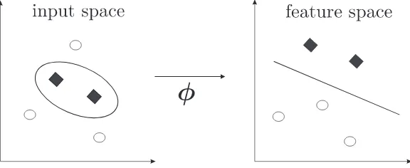
Figure 1.1: Linearly inseparable data in the input space can become linearly separable
by mapping them viaφinto a higher dimensional feature space. Then a linear decision boundary in the feature space yields a nonlinear curve in the input space.
(Fig. 1.1). There is also a possibility that the original vector representation ofxincludes many irrelevant attributes. This may disorientate the training procedure from a solution able to successfully predict the unknown labels. Such undesirable situations can be avoided by an embedding of the data into an appropriate feature space which encodes a prior knowledge about the problem and offers a representation with the suitable number of features.
As an example of how to explicitly incorporate our prior knowledge in the feature map-ping let us assume that the only relevant information about a given task is contained in monomials of degree 2 formed out of the attributes of x. Then, taking for the sake of simplicity the dimensionality of the input space to be equal to 2, we have the following embedding
x= (x1, x2)−→φ(x1, x2) = (x21, x22, x1x2) .
In the case of an input space of dimensionality equal tonone can construct the feature space of all possible monomials of degree exactly equal todby an analogous procedure. The dimensionality N of such a feature space is then given by the formula
N = n+d−1
d
!
= (n+d−1)!
d!(n−1)! .
It is apparent that a large number of attributes n in combination with a large value of
dwill eventually lead to an explosion in the number of dimensions of the feature space making the explicit construction of such a feature mapping computationally impractical.
1.3
Implicit Mapping via a Kernel
space produce functions assigning labels to the unseen patterns which are of the type
f(x) =
N
X
i=1
wi·φi(x) +b . (1.2)
Assuming again that the weight vector wadmits a dual representation with respect to the transformed training data (1.2) becomes
f(x) =
l
X
i=1
αiyiφ(xi)·φ(x) +b . (1.3)
The previous relationship involves an explicit non-linear mapping φ from the space
X which the training data and the test point live in into the feature space H. The functionf(x) is constructed by a linear machine working in the feature space aiming at classifying the training data by means of a hyperplane. The linear surface performing the classification in H corresponds to a non-linear surface in the input space. Notice that here the inner product of the transformed instances plays the role of the similarity measure. Equation (1.3) suggests that explicit knowledge of the feature mapping would be obsolete if one was able to compute directly the inner product involving the training data and the test point in the feature space. The previous observation that only the knowledge of the inner product suffices if we are interested in constructing appropriate classification functions in the feature space motivates the following definition of the kernel function.
Definition 1.1. A kernel is a functionK:X xX→R, such that for allx, x′ ∈X K(x,x′) =φ(x)·φ(x′)
withφa mapping from X to an inner product feature space H.
The kernel function K takes as arguments any two points x and x′ and returns a real number measuring the similarity of their images in the feature space. Thus, the kernel may be viewed as a similarity measure “transformed” by the feature mapping. This becomes more obvious if we consider in the place of φ the identity function which defines a kernel coinciding with the inner product in the input space
K(x,x′) =x·x′ .
We assumed earlier that the weight vector can be decomposed as a linear combination of the transformed patterns thus giving rise to the dual representation. By taking into account the definition of the kernel (1.3) can be equivalently rewritten as
f(x) =
l
X
i=1
The decision rulef(x) entails at mostlkernel evaluations which are as many as the data contained in the training set. A mere observation of (1.4) reveals that the introduction of the kernel eliminates any complications in the computation of the decision rule f(x) stemming from the possibly large dimensionality of the feature space. Therefore, the number of operations involved in the evaluation of the kernel function are not necessarily controlled by the number of features, thereby reducing the computational complexity of the decision rule.
Let us attempt to illustrate how it is possible by constructing directly the kernel to avoid the operations involved in the evaluation of the inner product in the feature space associated with an explicit description of the feature mapping. For our demonstration we choose to evaluate the square of the inner product in the input space and investigate the possibility that it constitutes a kernel. Each vector participating in the inner product is analysed in its components and the square of the product is computed as follows
(x·x′)2 =
n
X
i=1 xix′i
!2 =
n
X
i=1 xix′i
!
n
X
j=1 xjx′j
=
n
X
i=1 n
X
j=1
xixjx′ix′j = (n,n)
X
(i,j)=(1,1)
(xixj) x′ix′j
.
From the preceding analysis we can conclude that the square of the inner product con-stitutes a kernel which performs a mapping into a feature space consisting of monomials of degree exactly 2
φ(x) = (xixj)((n,ni,j)=(1) ,1) .
Notice that the features xixj for i 6= j appear twice leading to a double weight in comparison to the weight of x2
i. In order to build a space the features of which are the
monomials up to degree 2 we have to add a constant parameterc to the inner product before raising it to the second power. The resulting kernel is analysed as follows
(x·x′+c)2 =
(n,n)
X
(i,j)=(1,1)
(xixj) x′ix′j
+
n
X
i=1
√ 2cxi
√
2cx′i+c2 .
The transformationφcorresponding to the above kernel comprises as features in addition to monomials of degree 2 monomials of degree 1 and 0 which are weighted according to the parameterc.
1.4
Characterisation of Kernels
explicit mapping which was known to us and then infer from it how the same result could be derived by employing only quantities associated with the input space. It would be very useful, however, to identify the properties characterising a kernel since this would enable us to directly construct kernels without even knowing the explicit form of the feature mapping. From the definition of the kernel it is easily derived that every kernel is symmetrical in its arguments
K(x,x′) =φ(x)·φ(x′) =φ(x′)·φ(x) =K(x′,x) .
A second property of kernels comes from the Cauchy-Schwarz inequality which yields
K2(x,x′) = φ(x)·φ(x′)2
≤ kφ(x)k2φ(x′)
2
=K(x,x)K(x′,x′) .
Nevertheless, none of these properties suffice to ensure that the function under consid-eration is indeed a kernel. A function is certainly a kernel only if it represents an inner product defined in a feature space to whichx∈X is mapped viaφ. Hence, we have to identify the conditions that guarantee the existence of such a mappingφ.
Let us consider a finite input space X = (x1,x2, . . . ,xl) and suppose K(x,x′) is a
symmetric function onX. Using this function we can construct a square matrix K the entries (i, j) of which are filled with the values that the function K assumes for every pair (xi,xj)
K = (K(xi,xj))l(i,j)=1 .
Since this matrix is furthermore symmetrical it can be decomposed as K = VΛVT, whereΛis a diagonal matrix with elements the eigenvaluesλi ofKandV an orthogonal
matrix with entries vij the columns of which are eigenvectors of K. Next we consider
the feature mappingφwhich mapsxi to a vector consisting of theith component of all
eigenvectors scaled by the square root of the accordingly indexed eigenvalues
φ:xi −→φ(xi) =
p
λ1vi1, . . . ,
p
λlvil
. (1.5)
In order to perform the above mapping we make the assumption that the eigenvalues are non-negative. Looking at (1.5) we realise that with such a mapping we are able to recover any entry kij of the matrixK if we work out the inner productφ(xi)·φ(xj)
φ(xi)·φ(xj) =
X
t,r δtr
p
λtvit
p
λrvjr =
X
t,r
vitΛtrvjr= VΛVT
ij =kij .
Here δij is Kronecker’s δ. This implies that K(x,x′) is indeed a kernel function
corre-sponding to the feature mappingφ. The constructed feature space with dimensionality at mostlis spanned by thelvectorsφ(xi), i= 1, . . . , lwhich resulted from the mapping.
φ(xi)’s
z=
l
X
i=1
visφ(xi) .
The squared norm of z is given by
kzk2 = X
i
visφ(xi)
!
·
X
j
vjsφ(xj)
= X
i,j
visvjskij
= VTKV
ss= Λss =λs .
Since such a squared norm of a vector is a non-negative quantity the eigenvalues of K must be non-negative. The above discussion concerning the eigenvalues of K leads to the following proposition.
Proposition 1.2. Let X be a finite input space with K(x,x′) a symmetrical function with respect to its arguments. Then K(x,x′) is a kernel function if and only if the matrix
K= (K(xi,xj))l(i,j)=1
is positive semi-definite.
In the above discussion that led to Proposition1.2we studied the eigenvalue problem of a kernel matrix K constructed by the values that the kernel function assumes on every possible pair drawn from a finite number of points. More specifically, we examined any restrictions that may hold for the eigenvaluesλsassociated with the following eigenvalue
problem
Kvs=λsvs .
An extension of this eigenvalue problem in order to cover the case of an infinite input space X is
Z
X
K(x,x′)ψ(x′)dx′ =λψ(x) .
This is an eigenvalue problem in an infinite dimensional space where the role of the eigenvectors is played by the eigenfunctions ψ. In analogy with Proposition 1.2 the following theorem [42] is concerned with the conditions that K should fulfill in order for it to be a kernel function.
Theorem 1.3. (Mercer) LetX be a compact subset of Rn. Suppose K is a continuous symmetric function such that the integral operator TK :L2(X) →L2(X) defined by
(TKf)(x) =
Z
X
K(x,x′)f(x′)dx′
is positive, meaning that
Z
XxX
for all f ∈L2(X). Here L2(X) is the space of measurable functions over X which are
square integrable. Let us denote by ψi ∈L2(X) the normalised (kψikL2 = 1) orthogonal
eigenfunctions of TK associated with the eigenvalues λi ≥0. Then, ∞
X
i=1
λi <∞
and K(x,x′) can be expanded as a uniformly convergent series
K(x,x′) =
∞
X
i=1
λiψi(x)ψi(x′) . (1.7)
Observe that the condition for positivity of the operator TK can be reduced to the
conditions for positive semi-definiteness of a kernel matrix K = (K(xi,xj))l(i,j)=1. In
order to obtain the latter we have to choose in the place of the functionsf(x) appearing in (1.6) a weighted sum of delta functions at the points xi, i= 1, . . . , l. The weights of
the delta functions will form a vector v for which
vTKv≥0
holds true. We can assert the converse too, i.e. if the positivity of TK is violated then
we can approximate the integral appearing in (1.6) by a sum over a sufficiently large number of appropriately chosen points which will be negative. This proves that Mercer’s theorem provides the general conditions for a function to be characterised as a kernel subsuming the specific case of a finite input space.
Mercer’s theorem suggests the feature mapping
x= (x1, . . . , xn)−→φ(x) = (ψ1(x), . . . , ψj(x), . . .)
into the feature spaceHwhich is the Hilbert spacel2(λ) of all sequencesz= (z1, z2, . . . , zi, . . .) such that
kzk2 =
∞
X
i=1
λizi2 <∞ ,
where the inner product of sequences xand z is defined by
x·z=
∞
X
i=1
λixizi .
This is so since the inner product of two feature vectors satisfies
φ(x)·φ(x′) =
∞
X
i=1
In order for the kernel to be represented an infinite number of eigenfunctions may be actually required or it may be the case that the infinite series reduces to a finite sum due to the vanishing ofλi forisufficiently large. In the latter case involving a space of finite
dimensionality NH, where ψi’s form an orthonormal basis, K(x,x′) can be considered
as an inner product inRNH. SinceK(x,x′) =φ(x)·φ(x′) the components entering the inner product will be determined by the induced mappingφon the pointsx
φ:x−→(ψi(x))Ni=1H .
Even when the induced space is of infinite dimensionality we can approximate the kernel functionKwithin some accuracyǫif a space of an appropriate dimensionalitynis found into which the points are mapped. If the eigenvaluesλi, i= 1, . . . , n, . . . are sorted in a
non-increasing order and a mapping
φ:x→(ψi(x), . . . , ψn(x))
is performed we can achieve that
|K(x,x′)−φ(x)·φ(x′)|< ǫ .
The features ψi entering (1.7) have the additional property that they are orthonormal.
It seems that the property of orthogonality is inherent in Mercer’s theorem and it is related to the eigenfunctions of the integral operator TK constructed for the specific
kernel function. Note that this is not required and we may optionally allow mappings that do not involve orthonormal features. To such a case belongs the kernel which corresponds to all the monomials of second degree. In addition to the flexibility that we have shown as far as the orthogonality is concerned we can also allow for a rescaling of the features
x= (x1, . . . , xn)→φ(x) = (b1φ1(x), . . . , bjφj(x), . . .) ,
where by b1, . . . , bj, . . . we denote the rescaling factors. We can recover the relation
φ(x)·φ(x′) =K(x,x′) if we define an altered inner product
x·z =
∞
X
j=1 λj b2 i
xjzj
wherex,zdenote any two points in the feature space. Employing the new definition we obtain
φ(x)·φ(x′) =
∞
X
j=1 λj b2 j
bjφj(x)bjφj(x′) =K(x,x′) .
decision rulef(x) written in terms of the values of the kernel function on pairs consisting of the training points xi and the test point x
f(x) =
l
X
i=1
αiyiφ(xi)·φ(x) +b= l
X
i=1
αiyiK(xi,x) +b .
If we define a vectorψ living inH to be a linear combination ofφ(xi), i= 1, . . . , l
ψ=
l
X
i=1
αiyiφ(xi) (1.8)
the decision rulef(x) can be equivalently expressed in the primal form
f(x) =
∞
X
i=1
λiψiφi(x) +b
with (1.8) linking the primal with the dual representation. We should remark here that the immediately preceding expression of f(x) which involves explicit mappings of the training and test points in the feature space requires the summation of as many terms as the dimensionality of the feature space as opposed to the dual representation which contains onlylterms. In order to choose which of the two representations suits us most we have to weigh the size of the dataset against the dimensionality of the feature space. As we discussed earlier there are situations where the infinite sum in the above equation may be truncated without a significant error.
We conclude this section by pointing out that there is not a unique mapping of the data that leads to a given kernel. Mappings that are associated with different feature spaces even in terms of their dimensionality can result in the same kernel.
1.5
Examples of Kernels
The procedure described in Section 1.3for constructing kernels associated with embed-dings to feature spaces consisting of all the monomials of degree 2 can be extended to kernels representing the inner product of vectors the components of which are monomials of arbitrary degree d. Let us consider the dth order product (xj1xj2. . . xjd) constructed by attributes of the pointxin which the indicesj1, j2, . . . , jd run over 1, . . . , n, wheren
is the dimensionality of the original space. Next we form a vectorφ(x) the attributes of which are all thedth order products which result after exhausting the combinations on the values of the indicesj1, . . . , jd. We carry out the inner productφ(x)·φ(x′) which
φ(x)·φ(x′) =X
j1
· · ·X
jd
xj1xj2. . . xjdx′j1x
′ j2. . . x
′ jd
=X
j1
xj1x′j1· · ·
X
jd
xjdx′jd=
X
j xjx′j
d
= x·x′d
.
This means that the inner product of vectors under a mapping which transfers them to a space formed by all the monomials of degreed corresponds to the kernel
K(x,x′) = (x·x′)d .
Since the surface that classifies the examples into two categories is a polynomial curve we call this kind of kernels polynomial kernels. For d = 1 we obtain a special case of a polynomial kernel which is the linear kernel K(x,x′) =x·x′. We have seen before that a space the features of which are monomials up to degree 2 is endowed with the inhomogeneous polynomial kernelK(x,x′) = (x·x′+c)2. Generalising this result to a space consisting of all the monomials up to degreedwe end up with the following kernel
K(x,x′) = (x·x′+c)d .
Apart from the polynomial kernels it is worth mentioning the general category of Radial Basis Function (RBF) kernels. Their characteristic is that they are written in the form
K(x,x′) =g(d(x,x′)) ,
wheregdenotes a function taking as an argument a metricdonXand mapping it to the space of nonnegative real numbers. The most common metric applied to the points x and x′ is the Euclidean distance d(x,x′) =kx−x′k=p(x−x′)·(x−x′). A known
kernel falling into this category is the Gaussian kernel [2]
K(x,x′) = exp −kx−x′k
2
σ2
!
,
where σ is a positive parameter. Since the value of the Gaussian kernel depends only on the vectorial difference of 2 points it has the property of being translation invariant implying that K(x,x′) =K(x+x0,x′+x0). All the above mentioned kernels share
Elements of Statistical Learning
Theory
2.1
The General Inference Model
Pattern recognition can be viewed as a problem of extracting knowledge from empirical data. The main approach until the 60’s for estimating functions using experimental data was the parametric inference model which is based on the assumption that the unknown functions can be appropriately parametrised. Then the experimental data are used in order to determine the unknown parameters entering the model. Fisher [16] was one of the pioneers in this direction who suggested the maximum likelihood approach as a method of solving problems cast in this form. The original belief that these methods could prove successful in real-world problems originated from the Weierstrass approximation theorem stating that any continuous function defined in a finite interval can be approximated to any level of accuracy by polynomials of an appropriate order. This belief was further reinforced by the fact that whenever an outcome is the result of a large number of interacting independent random factors the distribution underlying their sum can be described satisfactorily by the normal law according to the Central Limit Theorem.
The drawback of the parametric inference model, however, is that its efficiency is strongly dependent on the dimensionality of the space which the data live in. In particular such methods break down in cases involving high-dimensional data spaces. In such spaces the existence of singularities in the function to be approximated is very probable. The existence of only a small number of derivatives for such non-smooth functions demands polynomials of degree increasing with the number of dimensions, if polynomial approx-imator functions are used, in order to achieve an acceptable level of accuracy. This phenomenon is characterised as “the curse of dimensionality”.
In the opposite direction lies the general analysis of statistical inference initiated by Glivenko, Cantelli and Kolmogorov. Glivenko and Cantelli proved that if one uses a very large number of independent observations which follow some distribution then, indepen-dently of the actual probability distribution governing the data, one can approximate it to any desired degree of accuracy. Kolmogorov’s contribution was the establishment of bounds concerning the rate of convergence to the actual distribution. This theory which makes no assumption about the underlying distribution was called the general inference model as opposed to the particular (parametric) one.
Both approaches have the common goal of finding the function that describes well unseen data by exploiting only a finite data sample. A learning machine that takes as input this sample of data and produces a function able to explain well unseen data is said to have good generalisation ability.
By generalising the Glivenko-Cantelli-Kolmogorov results a theory was developed [60,61] which links the training procedure of the learning machine involving a finite training sample with its ability to produce rules that work well on examples to be presented to it in the future. According to this theory the only relevant quantity related to the training process is the number of examples that the machine failed to explain based on the rule that has been generated. These wrongly explained examples are characterised as training errors. Central to this theory is the Empirical Risk Minimisation (ERM) principle which associates the small number of training errors with the good generalisation ability of the learning machine.
There are two main issues that this theory should address. The first involves the identifi-cation of necessary and sufficient conditions under which the ERM principle is consistent. Consistency of the ERM principle means that the estimated function is able to approach the best possible solution within a given set of functions with an increasing number of observations. The second issue involves quantitative criteria associated with the solution found. For example, we would like to know what the probability of error on unknown examples is when we have already estimated the function that minimises the training errors in a dataset of a given size and how much this probability differs from the one associated with the optimal choice among functions belonging to a given set.
the rate of convergence led to bounds which depend on the VC dimension, the number of training errors and the size of the dataset presented to the machine during the training phase.
As the ERM principle suggests one should be interested in estimating a function that makes a small number of errors on the training set because this would automatically imply a small error rate on unseen data (test error). It is expected that if the learning machine employed has at its disposal a large set of candidate functions then it becomes easier to find the function that leads to the smallest possible training error. There exist bounds that constrain the probability of error simultaneously for all the functions in the set and involve quantities like the number of training errors and the VC dimension of the set of functions. A larger VC dimension implies a greater ability of the functions contained in the set to explain the data leading possibly to smaller training errors. The presence of the VC dimension in the bounds can influence the minimum number of errors on unseen data (i.e. the risk suffered). This is an interesting property of the bounds which will be investigated at a later stage of our analysis.
2.2
Learning from Examples
The learning model that will be considered consists of three main parts:
1. The generator of the training instances.
2. The target function (supervisor) operating on the training instances.
3. The learning machine.
The generator is thought of as being a source the statistical properties of which remain invariant during the procedure. Its role is to generate a numberlof instancesxbelonging to an n-dimensional spaceXwhich are independently drawn and identically distributed (i.i.d.) according to some unknown distribution. The target function (supervisor), which is unknown to us as well and remains the same as long as the training takes place, receives these instances as input and produces an outputybelonging to a spaceY which is visible to us. The learning machine tries to estimate the target function employing as the only source of knowledge the instance-target pairs
(x1, y1),(x2, y2), . . . ,(xl, yl) .
Nevertheless, one should distinguish the case of constructing a function performing well on the data from the case of ending up with a function lying close to the target function with respect to some metric. Obviously, the latter is a stronger requirement which subsumes the case of imitating the behaviour of the oracle.
2.3
Minimising the Risk Functional
In the previous section we saw that during the training phase the learning machine constructs a function which operates on the data. As a matter of fact the machine chooses the appropriate member from a class of functions H ⊂ YX referred to as the
hypothesis class. YX denotes the set of all functions which map the input spaceX onto the output space Y. The selection of the function f(x), which is called a hypothesis, can be done according to some predetermined criteria. To make this more formal we define the following functional
R=R(f(x)) ,
which depends on the set of admissible functionsf(x). Among these the functionf0(x)
has to be found which minimises R which for this reason will be referred to as the risk functional. If we consider that the samples are generated according to a probability distributionF(x, y) then the risk functional can be expressed as the expectation
R(f(x)) = Z
L(y, f(x))dF(x, y) .
As we have mentioned before the probability distribution is unknown and minimisation can be performed only by employing the empirical data available during the training process. If we call A the algorithm implemented by the learning machine then for a given samplez= (x, y) and a hypothesis classHwe assume thatAproduces hypotheses belonging toH, coded formally as A(z, H)∈H.
The function L(y, f(x)) appearing in the integral is known as the loss function and is a measure of the discrepancy between the output produced by f and the target. Additionally, we have to impose that the loss function be integrable for anyf(x) ∈H. This loss function can be parametrised bya∈Λ allowing us to distinguish the admissible functions belonging to the same hypothesis class. Notice that the set Λ which the parametera takes values from is connected to the admissible set of functions. In other words we establish a correspondence a → fa between elements a of the set Λ and
functionsfa∈H. UsingQ(z, a) instead ofL(y, f(x)) the risk functionalR(fa) becomes
the functionR(a)
R(a) = Z
Q(z, a)dF(z) . (2.1)
In the literature we come across three basic problems, namely the problem of classifica-tion, the problem of regression and finally that of density estimation. In the simplest problem, that of classification, an instance is generated according toF(x). The supervi-sor classifies the new instance to one ofkclasses according to the conditional probability
F(ω|x), whereω∈ {1,2, . . . , k}. For the special case of binary classification the number of classes is fixed to two. In the regression problems there is a functional relationship or more generally a stochastic dependency linking eachxto a scalarywhich takes values in the range (−∞,∞). This dependency is described by the probabilityF(y|x) of y given x. In the problem of density estimation we seek to determine the probability density
p(x, a0) among the set of admissible densities p(x, a), a ∈ Λ that corresponds to the
unknown distribution F(x) which generated the observed instances x. The difference from the cases of classification and regression is that the supervisor providing the values of y is missing, soz coincides with x.
Various loss functions have been proposed depending on the nature of the problem. For example, for binary classification problems the 0-1 loss has been adopted which is described by
L0−1(ω, φ(x, a)) =
0 if ω =φ(x, a) 1 if ω 6=φ(x, a) .
The argument φ(x, a) in the loss function denotes the prediction of the machine for a given x on the basis of the function selected from the hypothesis class. The loss function in the binary classification problem is a set of indicator functions that take only two values, either zero or one. For regression the squared loss is commonly used which is given by
L2(y, φ(x, a)) = (y−φ(x, a))2 .
The loss function in this case does not take values from a finite set but instead can be equal to any nonnegative number. For the density estimation problem the loss function
L(x, φ(x, a)) =−lnp(x, a)
is used which takes values in the range (−∞,∞). Such a choice of the loss function is motivated by the fact that the corresponding risk coincides, apart from a constant, with the Kullback-Leibler (KL) distance between the approximate density p(x, a) and
p(x, a0). The minimum value of the risk R(a0) coincides with the entropy of the
distri-bution associated withp(x, a0).
As suggested by the ERM principle instead of minimising the risk function one can minimise the empirical risk
Remp(a) = 1 l
l
X
i=1
For the special case of binary classificationQ(zi, a) takes values from the set{0,1}. Let
us assume that the minimum of the risk is attained atQ(z, a0) whereas the minimum of
the empirical risk atQ(z, al). We will considerQ(z, al) as an approximation ofQ(z, a0)
and try to identify the conditions under which the former converges to the latter.
It is worth pointing out here that since the machine has a restricted set of functions at its disposal the best that we can expect from the algorithm is to estimatea0 as
a0= arg min a∈ΛR(a) .
Nevertheless, the best estimate lies among the set of all possible functionsYX mapping the space X onto Y and for that estimate the risk acquires its minimum valueRmin.
Previously in our discussion we emphasised the importance of the richness of the hy-pothesis class Λ described by the VC dimension as a decisive factor on which the gen-eralisation ability of the machine depends. The choice of Λ brings forward a dilemma known as the approximation-estimation or bias-variance dilemma. In order for this to become apparent the difference of the risk due to any function corresponding to the parametera∈Λ and the minimum possible value of the riskRminhas to be decomposed
as
R(a)−Rmin = (R(a)−R(a0)) + (R(a0)−Rmin) .
The second term on the r.h.s. is characterised as the approximation error. Apparently, as the set of admissible functions is enlarged the feasibility of a function being closer to the best estimate increases. The same does not apply for the first term called the estimation error. In this case a larger hypothesis class means that the risk incurred by any function in the set will be probably further away from the minimum risk incurred by
a0. Therefore, the most successful choice of Λ, that is, the one that containsaminimising
the l.h.s. can only result as a trade-off between the approximation and the estimation error.
2.4
Consistency of the Learning Process
The quality of an algorithm A can be judged by its ability to converge to functions (hypotheses) which lead to risks lying close to the minimum of the risk function attained at a0 ∈ Λ. The algorithm should succeed in that task only by means of the training
sample made available to it. The construction of the hypothesis is suggested by the appropriate induction principle which in our case is ERM. Through that principle A produces a solution hypothesisal ∈Λ, depending on the sizelof the training set, which
leads to Q(z, al) from which an expected risk R(al) could have been estimated if the
distribution generating the sample was known. Thus, the expected risk R(al) has to
completion of the training procedure. There are two fundamental questions that can be raised. What is the relation between the empirical risk and the expected risk for the solution found? Is it possible for the expected risk to approach the smallest feasible value for functions belonging to the set Λ? These matters will be addressed by the study of the consistency of the ERM principle.
Definition 2.1. The principle of empirical risk minimisation is consistent for the set of functions Q(z, a), a ∈ Λ and for the probability distribution function F(z) if the following two sequences converge in probability 1 to the same limit
R(al)
l→∞
−→
P ainf∈ΛR(a) (2.2)
Remp(al)
l→∞
−→
P ainf∈ΛR(a) . (2.3)
The first of the two equations requires that in the limit of an infinite dataset size provided to the machine the sequence of achieved risks on the basis of the functions constructed tends to the minimum one. The second equation requires that in the same limit the sequence of empirical risks estimated on the set of training data given to the machine also tends to the same value.
From the Definition2.1it is evident that consistency is a property of the functions that the machine implements and the distribution that generates the data. We would like consistency to be achieved in terms of general criteria characterising the whole class of admissible functions and not specific members of the class. However, even a set of inconsistent functions can be rendered consistent by adding to it a function which minimises the loss Q(z, a). Then, it is easily understood that the minimum of the empirical risk is attained at this function which also coincides with the minimum of the expected risk. In order to tackle such kind of situations we have to exclude functions from the set of admissible ones that lead to trivial satisfaction of the consistency criteria. This can be done by reformulating the definition of the ERM consistency as follows.
Definition 2.2. The ERM principle is strictly (non-trivially) consistent for the set of functions Q(z, a), a ∈ Λ and for the probability distribution function F(z) if for any nonempty subset Λ(c), c ∈(−∞,∞) of this set of functions such that
Λ(c) =
a: Z
Q(z, a)dF(z)≥c
the minimum of the empirical risks defined over any such subset Λ(c) tends to the minimum expected risk for functions of this subset
inf
a∈Λ(c)Remp(a)
l→∞
−→
P a∈infΛ(c)R(a) .
1Convergence in probability means that for all ǫ >0 we have P{|R(αl)−infα
∈ΛR(α)|> ǫ}
l→∞ −→ 0 andP{|Remp(αl)−infα∈ΛR(α)|> ǫ}
l→∞
If the ERM principle is strictly consistent then (2.2) of Definition 2.1 is automatically fulfilled.
We now give an example in which the first limit in Definition2.1holds whereas the second is violated. To illustrate this we consider the set of indicator functions Q(z, a), a∈ Λ. To our class belong only functions Q which take the value zero at a finite number of intervals which as a total have measureǫand are equal to one elsewhere. The parameter
adistinguishes the functionsQaccording to the specific intervals at which their value is equal to zero. If a number of examples z1,z2, . . . ,zl is supplied to a learning machine
working on the basis of ERM principle it will favour the solutions a for which the functionsQbecome zero at the training points. Consequently, for this class of functions we have
Remp(al) = inf a∈Λ
1
l l
X
i=1
Q(zi, a) = 0 .
The expectation of the risk for any function in the set and therefore for the function al
constructed by the machine is given by
R(a) = Z
Q(z, a)dF(z) = 1−ǫ . (2.4)
Combining the above two equations we obtain
inf
a∈ΛR(a)−Remp(al) = 1−ǫ .
Furthermore, due to (2.4) it obviously holds that
R(al)− inf
a∈ΛR(a) =
Z
Q(z, al)dF(z)−inf a∈Λ
Z
Q(z, a)dF(z) = 0 .
We conclude that although the expectation of the risk converges to the smallest possible in the set the same does not hold for the empirical risk. Therefore, for that class of functions the ERM principle is not consistent.
The ERM consistency demands some asymptotic criteria that must be met in order for the solution constructed in terms of empirical data to converge to the optimal one. Notice that the optimal solution depends on the real distribution producing the data. We can get some intuition about what is needed to satisfy the criteria by studying another example in which an induction principle somewhat different from the ERM one is used.
function can be rewritten as follows
R(a) = Z
Q(z, a)dF(z) = Z
Q(z, a)p(z)dz ,
where p(z) is the density function corresponding to the distribution F(z). Further-more, we demand that the loss function be uniformly bounded by a positive constant
B (|Q(z, a)| ≤ B). This is true in the binary classification since Q(z, a) are indicator functions and take the value of either 1 or 0. Let us also assume that the densitypl(z)
estimated from the data converges in probability to the true density p(z) in the L1
metric, i.e.
Z
|pl(z)−p(z)|dz
l→∞
−→ P 0 .
We also consider the empirical riskR⋆emp
Remp⋆ (a) = Z
Q(z, a)pl(z)dz (2.5)
associated with an induction principle different from the usual one. We would like to emphasise that the above modified empirical risk is generally expected to be different fromRempsince the empirical density pl is not necessarily concentrated on the observed
data but may assume non-zero values elsewhere. As a result the integral in (2.5) does not always reduce to a finite sum. With these assumptions and the requirement in mind that Q be bounded we will prove that the function Q(z, al) which minimises R⋆emp(a)
defined in terms of the estimator pl converges to the optimal one Q(z, a0) among all
functions minimising R(a). Constructing the supremum over all the functions in the class we obtain
sup
a∈Λ
Z
Q(z, a)p(z)dz− Z
Q(z, a)pl(z)dz
≤
sup
a∈Λ
Z
|Q(z, a)| |p(z)−pl(z)|dz
≤B
Z
|p(z)−pl(z)|dz
l→∞
−→
P 0 . (2.6)
Thus, with the expectation taken over the actual distribution the expected risk converges in probability for all functions in the class simultaneously to the risk with the expectation now taken over the empirical probability estimator. From the previous relationship it can be derived that for anyǫand η there exists a number of examples l′(ǫ, η) such that for any l > l′(ǫ, η) with probability 1−η
Z
Q(z, al)p(z)dz−
Z
Q(z, al)pl(z)dz < ǫ , (2.7)
−
Z
Q(z, a0)p(z)dz+
Z
hold. SinceQ(z, al) is the minimiser of R⋆emp the following is true
Z
Q(z, al)pl(z)dz≤
Z
Q(z, a0)pl(z)dz . (2.9)
Combining (2.7), (2.8) and (2.9) we obtain that with probability 1−η
Z
Q(z, al)dF(z)−
Z
Q(z, a0)dF(z)<2ǫ (2.10)
holds true. Summing up, we can assert that the minimisation of the induction principle (2.5) under the condition of boundedness of Q(z, a) and the convergence of densities guarantees that the risk estimated withQ(z, al) converges in probability to the smallest
possible in the limit of infinite data sample size. From (2.6) it is apparent that we do not need the empirical density to converge to the true one, but it suffices instead that
sup
a∈Λ
Z
Q(z, a)p(z)dz− Z
Q(z, a)pl(z)dz
l→∞
−→ P 0 .
If we are interested only in the binary classification, Q(z, a) are indicator functions and the integral R
Q(z, a)p(z)dz can be interpreted as the probability P(Aa) of the event Aa ={z:Q(z, a) = 1} with respect to the distribution density p(z). In an analogous
way the integral R
Q(z, a)pl(z)dz can be interpreted as the probability Q(Aa) of the
same event Aa only this time with respect to the empirical density pl. The following
theorem due to Scheffe relates the difference of densities in L1 metric to the supremum
of the difference of the corresponding probabilities:
Theorem 2.3. Let p(x) and q(x) be densities, let F be Borel sets of events A and let
P(A) =R
Ap(x)dxandQ(A) =
R
Aq(x)dxbe probabilities of the setA∈ F corresponding
to these densities. Then
sup
A∈F|
P(A)−Q(A)| ≤1/2 Z
x|p(x)−q(x)|dx .
An immediate consequence of the theorem is that convergence of densities in the L1
metric leads to convergence over the set of all events of the corresponding probabilities. This implies that convergence of the densities is a stronger condition to impose than convergence of the probabilities, especially if one is interested in the convergence over a subset F⋆ of the set F of events. Therefore, one should move in the direction of
identifying conditions under which this holds true. At this point we should note that apart from asymptotic bounds one can acquire non-asymptotic ones as that of (2.10) on the generalisation of the learning machine depending only on a finite number of observations.
the minimal value of the risk function (2.1) can be attained. For this to take place we require that the loss functions be bounded and non-negative and furthermore that the empirical risk estimatorνl(A) of an eventAconverge in probability to the corresponding
true probabilityP(A)
sup
A∈F⋆|
P(A)−νl(A)|
l→∞
−→ P 0 .
Notice here that convergence holds for all the events belonging to a subset F⋆ of F.
Indeed, it can be proved that minimisation of the empirical risk produces a sequence of values R(al) that tend in probability to the minimal value of the risk for increasing
numbers of observations.
2.5
Empirical Processes
From what has preceded a connection was revealed between the consistency of the em-pirical risk minimisation principle and the convergence of the emem-pirical risk estimator of any event in a set to its true probability. We consider the sequence of random variables
ξl= sup
a∈Λ
Z
Q(z, a)dF(z)−1
l l
X
i=1
Q(zi, a)
.
Here, we make again the hypothesis that a number of examples l were independently generated by the same distribution F(z). We call this sequence which depends both on
F(z) and on the loss functionQ(z, a) a two-sided empirical process. As we remarked in the beginning of the section the relation to the consistency of ERM principle motivates us to investigate the conditions under which the empirical process converges in probability to zero, that is
P
( sup
a∈Λ
Z
Q(z, a)dF(z)−1
l l
X
i=1
Q(zi, a)
> ǫ ) l→∞
−→ 0 . (2.11)
The above relation describes the uniform convergence of means to their expectations. It is called uniform because it is taken over the set of all admissible functions. One can also consider the one-sided empirical process defined as
ξ+l = sup
a∈Λ
Z
Q(z, a)dF(z)− 1
l l
X
i=1
Q(zi, a)
!
+ ,
where
(u)+=
In analogy to the uniform two-sided convergence the uniform one-sided one takes place if
P
( sup
a∈Λ
Z
Q(z, a)dF(z)−1
l l
X
i=1
Q(zi, a)
!
> ǫ
)
l→∞
−→ 0 . (2.12)
If the set of Q(z, a), a ∈ Λ is chosen to be the set of indicator functions then the relations (2.11) and (2.12) are interpreted as uniform convergence of frequencies to their probabilities.
According to the law of large numbers if the set of admissible functions contains only one element then the sequence of means converges always to the expectation of the random variable for an increasing number of examples. Specialising this to the binary classification which we are interested in we consider a hypothesis class containing a single indicator functionQ(z, a⋆) with a⋆ denoting here a fixed event. The Bernoulli theorem verifies then that for l → ∞ the frequencies converge to the probability of the event
Aa⋆ ={z :Q(z, a⋆)>0}
P{|P{Q(z, a⋆)>0} −νl{Q(z, a⋆)>0}|> ǫ}l−→→∞0
whereνl{Q(z, a⋆)>0}is used to denote the frequency of the event. In addition to the
previous asymptotic bound Chernoff’s inequality [12]
P{|P{Q(z, a⋆)>0} −νl{Q(z, a⋆)>0}|> ǫ}<2 exp{−2ǫ2l}
yields bounds on the rate of convergence for a finite number of observations. The law of large numbers can be easily generalised to the case where the hypothesis class consists only of a finite number of functions N. Let Ak = {z : Q(z, ak) > 0}, k = 1,2. . . N
denote the set of N finite events. The uniform two-sided empirical process for finite events in the Bernoulli scheme is written as
max
1≤k≤N|P{Q(z, ak)>0} −νl{Q(z, ak)>0}| .
We can place upper bounds on the rate of convergence by application of Chernoff’s inequality which gives that
P
max
1≤k≤N|P{Q(z, ak)>0} −νl{Q(z, ak)>0}|> ǫ
≤
N
X
k=1
P{|P{Q(z, ak)>0} −νl{Q(z, ak)>0}|> ǫ}
≤2Nexp{−2ǫ2l}= 2 exp
lnN l −2ǫ
2
l
In order to derive convergence from (2.13) for any value of the parameterǫ
lim
l→∞
lnN
l →0
needs to hold. This is true for a finite number of elementsN in the hypothesis class.
The difficulties arise when the setQ(z, a), a∈Λ includes an infinite number of elements which is the case if aparametrises a functional space. The generalisation of the law of large numbers in the functional space is essentially the uniform convergence of the means to their expectations over the whole set of functions distinguished by the continuous variation of the parameter a. The discussion in the previous section suggested that the condition of uniform convergence is sufficient to guarantee the consistency of the ERM principle. The role of uniform convergence is to enforce the empirical risk to be close to the expected risk uniformly over all the functions in the set for a sufficiently large number of examples.
2.6
The Key Theorem of Learning Theory
In our earlier discussion it turned out that under the assumption of uniform two-sided convergence we can achieve the minimisation of the risk function through the minimi-sation of the empirical risk. The key theorem [65] introduces the uniform one-sided convergence as not only a sufficient but also as a necessary condition for the strict consistency of ERM.
Theorem 2.4. Let Q(z, a), a∈Λ, be a set of functions that satisfy the condition
A≤
Z
Q(z, a)dF(z)≤B .
Then for the ERM principle to be consistent, it is necessary and sufficient that the empir-ical riskRemp(a) converge uniformly to the actual riskR(a)over the set Q(z, a), a∈Λ,
in the following sense:
lim
l→∞P
sup
a∈Λ
(R(a)−Remp(a))> ǫ
= 0, ∀ǫ >0 .
We now turn to a discussion linking the one-sided with the two-sided convergence. In an attempt to reveal the relation we decompose the two-sided uniform convergence into the following two relations
lim
l→∞P
sup
a∈Λ
(R(a)−Remp(a))> ǫ
or
lim
l→∞P
sup
a∈Λ
(Remp(a)−R(a))> ǫ
= 0 . (2.15)
From this decomposition we recognise the one-sided convergence as the one of the two relations that must be satisfied for the validity of the two-sided convergence. It is possible that the two-sided convergence does not hold because the part (2.15) is violated but part (2.14) is valid leaving thus unaffected the one-sided convergence. Therefore the conclusion is that two-sided convergence is only a sufficient condition for ERM consistency. We can remark here that since we are interested only in the minimisation of the empirical risk the (2.15) part of the two-sided convergence which corresponds to the maximisation of the empirical risk can be violated.
2.7
Entropy and Other Related Concepts
The law of large numbers is valid in the case of a single event and can be readily generalised for a finite number of events. For the uniform law of large numbers to be applicable to functional spaces other tools are needed which will be constructed here. The idea for proving convergence in the case when the hypothesis class H comprises infinitely many events is based on the fact that not all of the events are distinguishable for a given samplez1,z2, . . . ,zl. Two events are treated as different if at least one example
in the sample which belongs to one event does not belong to the other. The number of distinguishable events, which are realised by equal in number effective functions selected from the hypothesis class, depends both on the sample size l and on the form of the functions in H and will be denoted by NΛ(z
1, . . . ,zl).
In what follows we will be concerned only with indicator functions Q(z, a). Let us take a sequence of vectors z1,z2, . . . ,zl produced independently by the same distribution.
We construct the followingl-dimensional binary vector
q(a) = (Q(z1, a), Q(z2, a). . . Q(zl, a)), a∈Λ
the components of which are the values of the loss functions at the points zk, k =
1,2, . . . , l in the sequence. For a fixed choice of the parametera=a⋆,q(a⋆) determines
one of the vertices of anl-dimensional unit cube. For the numberNΛ(z1, . . . ,zl) of such
vertices it holds that
NΛ(z1, . . . ,zl)≤2l .
The quantity 2l constitutes an upper bound on the number of different labellings that can be given to the sample z1,z2, . . . ,zl by means of indicator functions. We define
![Figure 4.3: Geometric illustration of the basic updates. If the projection falls withinthe segment [xi, ˜xi] either the IncreaseStep (Figure A.) or the DecreaseStep (FigureC.) takes place with τ0 < 1](https://thumb-us.123doks.com/thumbv2/123dok_us/8497374.346429/86.595.149.484.187.461/figure-geometric-illustration-projection-withinthe-increasestep-decreasestep-figurec.webp)