A preliminary evaluation of vision and laser sensing for tree trunk detection and orchard mapping

A preliminary evaluation of vision and laser sensing for tree trunk

detection and orchard mapping

Nagham Shalal

, Tobias Low

, Cheryl McCarthy

, Nigel Hancock

_{Faculty of Engineering and Surveying, University of Southern Queensland, Australia}

2

_{National Centre for Engineering in Agriculture, Toowoomba, Australia}

3

_{Control and Systems Engineering, University of Technology, Baghdad, Iraq}

{

NaghamJamilDawood.Shalal, Tobias.Low, cheryl.mccarthy, nigel.hancock

}

@usq.edu.au

Abstract

Mapping is a significant issue in mobile robot applications. Mobile robots can build a map or a model of the environment using different sen-sors. An orchard is a suitable agricultural envi-ronment for mobile robot applications since it is a semi-structured environment, where trees are planted in nominally straight rows. This pa-per presents a new method to extract features from the orchard environment using a camera and laser range scanner to create a map of the orchard. The map of the orchard is based on the detection of tree trunks. In this study, im-age segmentation and data fusion methods are used for feature extraction, tree detection and orchard map construction. Integration of both machine vision and laser sensor provides more robust information for tree trunk detection and orchard mapping. The resulting map composes of the coordinates of individual trees in each row as well as the coordinates of other non-tree objects detected by the sensors.

1

Introduction

In recent years, mobile robots have been introduced in different agricultural applications. The rapid develop-ment in sensors, communication and software techniques has encouraged many researchers and companies to de-velop automated agricultural robots to save labour and enhance safety. Navigation of mobile robot in agricul-tural environments consists of sensing the environment, mapping, localisation and obstacle avoidance.

Precise orchard maps are necessary for agricultural mobile robots localisation, path planning and navi-gation. Many researchers have developed automated or semi-automated agricultural mobile robots that can sense their environment and build a map of the environ-ment. The integration of different sensors for mapping increases the robustness of the map. Accurate environ-ment maps assist the mobile robot to easily estimate its

position and orientation at each time instant.

Orchards must be considered as semi-structured en-vironments because, although trees from the same kind are planted in nominally straight rows and the distances between the rows are almost equal (Figure 1), there re-mains significant spatial irregularity. The major problem in orchard mapping process is finding suitable features that are stable under different environmental conditions. In addition, orchards are frequently less tidy than illus-trated in Figure 1 with fallen debris (e.g. due to storm damage) and other obstacles, and local-scale mapping is often not constant over time. Whilst major features such as trees do not move, features change as trees grow, branches fall and other movable obstacles (e.g. animals) may also be present.

Figure 1: Example of tree rows in the orchard [Dream-stime, 2013]

localisation.

There are differences between the data acquired from the laser scanner and the camera image. The 2D laser scanner generates a single horizontal scan of the envi-ronment, whereas the camera generates an image. Laser scanner provides range and bearing data, while the cam-era primarily provides intensity and colour information. On the other hand, there are some common features in both types of data. For example, many corners and edges correspond to a sudden change in the range along the laser scan data and a sudden variation in the image in-tensity [Peynot and Kassir, 2010].

This work presents a new method for local-scale or-chard mapping based on tree trunk detection and util-ising modest-cost colour vision and laser-scanning tech-nologies. Fusion of data from the simultaneous use of these sensors improves object detection because the laser scanner can provide accurate ranges and angles of the objects, while the vision system can distinguish between tree trunks and other non-tree objects. The method seeks to achieve local-scale mapping appropriate as a component of robot navigation. Consideration of robot positioning is not the focus of this paper. The map ob-tained consists of the 2D location of the trees in the orchard which will be used later as a priori map with the measurements from the sensors to implement locali-sation, path planning, and navigation in the orchard.

This paper is organised as follows. Section 2 presents the recent studies published in the field related to this work. Section 3 describes the system architecture imple-mented in this study. Section 4 explains the proposed method for tree trunk detection using vision and laser sensors. Map construction method is described in Sec-tion 5. SecSec-tion 6 presents the experimental results and discussion. Finally, a summary of the significant conclu-sions and future work is presented.

2

Related Work

Mapping agricultural environments using mobile robots is a challenging subject. Several methods exist in the literature for feature extraction of the environment that construct a map of the environment to be used later for localisation and navigation of mobile robot. Another ap-proach is implementing Simultaneous Localization and Mapping (SLAM) algorithm which is used to build up a map within an unknown environment, while at the same time using this map to localise the mobile robot current location.

There are different methods to detect trees available in the literature. Several studies have been reported on the use of laser sensors for tree row detection in orchards and groves. Laser scanner data can be used to detect different components of the tree rows (e.g. trunk, stem, and canopy). Hansen et al. [2011] and Libby and

Kan-tor [2011] used the laser scanner to detect the dense canopy of the tree rows. However, Libby and Kantor [2011] found that the use of reflective tapes to detect the ends of the rows reduced processing time and enhanced row detection. Hamneret al. [2010] suggested a method to detect trunk and/or canopy of the trees for tree row recognition then Hough transform was implemented to extract point and line features to navigate the agricul-tural vehicle between the rows. In the study reported by Guivantet al. [2002], laser scanner was used to perform SLAM algorithm using the trunks of the trees as point features. Alternatively, techniques such as LIDAR can provide more-comprehensive canopy geometrical infor-mation and Rosell Poloet al. [2009] have demonstrated its use for the measurement of tree-row structure in or-chards, but not specifically for local mapping.

Researchers have also investigated the potential use of vision sensors for tree row detection in orchards. The use of vision sensors allows the extraction of different features from the environment such as colour, texture, shapes, and edges of the trees. A number of vision-based autonomous navigation systems have been developed for tree row following [Ayalaet al., 2008; Gao et al., 2010; Torres-Sospedra and Nebot, 2011]. These systems used different image segmentation and classification methods to extract the useful information for navigation and fo-cused on optimising the classification methods.

In some orchards, both vision camera and laser range scanner are used for mapping, localisation and au-tonomous navigation. Integration of both machine vision and laser scanner increases object detection capability. The work of Subramanianet al. [2006] presents an au-tonomous guidance system based on machine vision and laser radar. A combination of laser and vision sensors has been also used to develop SLAM algorithm [Cheein et al., 2011]. The SLAM algorithm is based on stems de-tection for the creation of agricultural maps using both laser range sensor and a monocular vision system.

Most of the SLAM algorithms have been focused in solving outdoor mapping for unknown and unstructured environments. SLAM has disadvantages of its processing time and computational requirements. The complexity of SLAM increases with the number of the landmarks and features in the map [Cheein et al., 2011]. However recent studies are seeking to address these issues.

based on tree trunk expected colour and the detected edges.

3

System Architecture

3.1

Robot Platform and Sensors

The platform used in the development of the tree trunk detection algorithm and orchard mapping is a CoroWare Explorer (CoroWare Inc., USA) which is designed to op-erate in outdoor conditions. It has a rugged articulated 4 wheel drive chassis with skid steering. It is equipped with an onboard computer running Ubuntu Linux op-erating system. Whilst this robot was used principally as a convenient sensor platform, a robot of this size, op-erating autonomously, could meet a major requirement in orchard management, namely simple inspection, e.g. to observe state of flowering, crop development, or dam-age following a storm event and carry little more that a camera and communications systems. Currently this is labour intensive task, especially in large orchards.

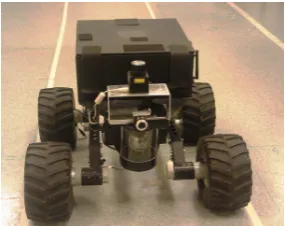
A camera-laser scanner combination is mounted on the robot platform. The camera used is a Logitech webcam Pro 9000 with 75◦view angle and 320×240 pixels image resolution. The laser range scanner used is a Hokuyo URG-04LX-UG01 scanning laser range finder with scan angle equal to 240◦and angular resolution equal to 0.36◦. The laser scanner is mounted on top of the camera and the camera-laser scanner combination is positioned at the front of the robot. Figure 2 shows a photo of the CoroWare Explorer platform with the onboard sensors.

Figure 2: CoroWare Explorer platform with the onboard sensors.

3.2

Camera-Laser Calibration

Camera calibration was performed to determine the in-trinsic parameters of the camera which include the focal lengthf c, the principal point coordinatescc, skew coeffi-cientalpha c, and the distortion coefficientskc. Camera calibration process was achieved using the Matlab cam-era calibration toolbox developed by Bouguet [2009].

The camera image is a projection of a 3D plane into 2D image plane and the laser signal is a 2D scan from the 3D world. It is critical to estimate the precise homo-geneous transformation between the coordinate systems

of the camera and the laser scanner to fuse the data ac-quired from these two sensors. Therefore, camera-laser calibration is implemented to determine the position and orientation of the camera relative to the laser scanner [Meng et al., 2010]. The camera-laser calibration was performed using the automatic camera-laser calibration toolbox developed by Kassir and Peynot [2010].

The results of camera-laser calibration toolbox are:

• The translation offset ∆ = [δx, δy, δz] , which is the

coordinates of the vector extending from the camera origin to the laser origin in the camera’s coordinate frame.

• The rotation matrixR= [φx,φy, φz], which

repre-sents the rotation between the camera and the laser frames about the axisx,y, andzrespectively. The secure mounting of the camera and laser scan-ner ensured that their relative positions were maintained during and after the camera-laser calibration.

3.3

Projection of Laser Points on the

Camera Image

The critical part of laser and camera data fusion is the projection of laser points onto the image plane of the camera. This projection required a prior camera-laser calibration to estimate the parameters of the transforma-tion between the the laser frame and the camera frame [Peynot and Kassir, 2010].

Projection of any laser point on the camera image is achieved in two steps:

• Transformation of the Cartesian coordinates of a point in a 3D space from laser frame to camera frame (laser-camera transformation).

• Projection from camera frame to the image plane.

Laser-Camera Transformation

Consider a point obtained by the 2D laser, defined by a range and a bearing angle, in a frame associated to the laser. This point can also be represented as a vector of 3D Cartesian coordinates in the laser frame Pl, and a

vector of 3D Cartesian coordinates in the camera frame Pc. These two vectors are related as follows [Peynot and

Kassir, 2010]:

Pl= Φ(Pc−∆) (1)

where ∆ = [δx, δy, δz] is the translation offset vector

and Φ is the rotation matrix defined by a set of three Euler angles R= [φx, φy,φz]. The rotation matrix Φ is

determined using the following equation:

Φ =





cycz cxsz+sxczsy sxsz−cxsycz −cysz cxcz−sxsysz sxcz+cxsysz

sy −sxcy cxcy



wheresi andci stand forsin(φi) and cos(φi)

respec-tively [Peynot and Kassir, 2010].

To achieve the laser-camera transformation, the 3D coordinates of any point with respect to laser frame is first calculated from the range r and bearing angle β of the point. Then the transformation from laser frame Pl= [Xl;Yl;Zl] to the camera framePc = [Xc;Yc;Zc] is

performed using Equation 1.

Projection to Image Plane

Consider a point P in space of coordinate vector Pc =

[Xc;Yc;Zc] in the camera reference frame. This point is

projected to the image plane according to the method implemented in the Matlab camera calibration toolbox by Bouguet [2009] as described in Equation 3 to Equa-tion 7 below. The normalized pinhole image projecEqua-tion is given by:

xn=

Xc/Zc Yc/Zc

=

x y

(3)

Let r2 = x2+y2. The new normalized point after including lens distortionkcisxdand is defined as follows:

xd=

xd(1) xd(2)

= (1 +kc(1)r2+kc(2)r4+kc(5)r6)xn+dx

(4) wheredxis the tangential distortion vector:

dx=

2kc(3)xy+kc(4)(r2_{+ 2x}2₎

kc(3)(r2_{+ 2y}2_{) + 2kc(4)xy}

(5)

Once the distortion is applied, the final pixel coordi-nates xpixel = [xp;yp] of the projection of the point P

on the image plane is determined as follows:

(

xp=f c(1)(xd(1) +alpha c∗xd(2)) +cc(1) yp=f c(2)xd(2) +cc(2)

(6)

Therefore, the pixel coordinate vector xpixel and the

normalized distorted coordinate vectorxd are related to

each other by:





xp yp

1



=K 



xd(1) xd(2)

1



 (7)

whereK is the camera matrix.

3.4

Simulated Environment

Simulated environment has been constructed for pre-liminary data collection and testing of the algorithm. This simulated environment can be considered as a small scale model of the real orchard and consists of simulated tree trunks constructed from mailing tubes with 900mm

height and 90mm diameter. The simulated tree trunks are placed in two rows with semi-equal distances between the simulated trees in the row and semi-equal distances between the rows as would be expected in an orchard as shown in Figure 3. In this simulated environment, we are assuming that no tall grass and 500mm of each simulated tree trunk is exposed above ground level.

Figure 3: The simulated environment.

4

Tree Trunk Detection Algorithm

The tree trunk detection algorithm developed in this study calculates the ‘rate of confidence’ for each object in the scene and determines whether it is a tree or non-tree. The rate of confidence is a value between 0 and 1 that is assigned to each tree trunk. The final rate of confidence ROCtree is calculated from laser scan data

and tree trunk colour and edges as shown in Figure 4. The tree trunk detection algorithm developed in this paper consists of two stages. In the first stage, laser scanner distinguishes between the candidate tree trunk and the non-tree objects. The candidate tree trunk then will further tested by the vision to decide if it is tree trunk or non-tree object.

4.1

Laser-Based Tree Trunk Detection

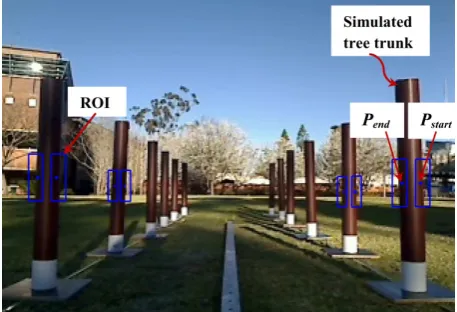
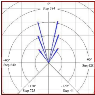
The algorithm first reads the scan data acquired from the laser scanner. Figure 5 shows a laser scan data in polar coordinates for the scene depicted in Figure 3, where the scan data starts from−120◦to 120◦in step of 0.36◦, the angular resolution of the laser scanner. Figure 6(a) con-tains the laser scan data as in Figure 5 but with the range data plotted on y-axis against the scan steps plotted on x-axis. The algorithm then detects the objects from the laser scan and determines their widthd. This is achieved by detecting the start and the end points (Pstart,Pend) of

Figure 4: Tree detection algorithm using camera and laser scanner.

data as shown in Figure 6(b). Each object is represented by a peak in Figure 6(a) anddis the number of steps be-tween the positive and negative spikes in the derivative data.

Figure 5: Laser scan data in polar coordinates.

The widthdof the object can be calculated from the polar representation of a single object in Figure 7 and it is described in the following equation

(a)

(b)

Figure 6: (a) Laser scan data (b) Derivative data.

d=r₁2+r₂2−2r1r2cos(∆β) (8)

wherer1andr2are the laser ranges atPstartandPend

of the object respectively, ∆β represents the difference between the start angleβ1 and the end angleβ2 of the

object as shown in Figure 7.

Figure 7: Object width determination from laser scan data.

depending on the type of the trees. The actual width of the tree trunk is less than the diameter of the tree trunk because the laser scanner does not have orthogonal view of the tree trunk and also due to the laser scanner mea-surement errors. The calculated µ and σ are used to determine the probability density function for the stan-dard normal distribution of the mean (pdf(µ)). For each scan, the algorithm determines the width of each object in the laser scan and calculates its probability density function pdf(d) and compares it with pdf(µ) to deter-mine the rate of confidence of the objectROClaser from

the laser scan. Thepdf(d) andROClaser are calculated

using Equation 9 and Equation 10 respectively:

pdf(d) = 1 σ√2πe

−(d−µ)2

2σ2 ₍₉₎

ROClaser = pdf(d)

pdf(µ) (10) TheROClaseris used to determine whether the object

is a candidate tree trunk or non-tree object from the laser scan depending on its value. A threshold value (ROCth)

for theROClaserthat distinguishes candidate tree trunk

from non-tree objects is determined empirically. The ROClaser of each object in the laser scan is compared

with the ROCth. If ROClaser of the object is greater

or equal to ROCth, then the algorithm considers this

object as a candidate tree trunk and projects itsPstart

andPendfrom the laser scan to the image, otherwise the

object is considered as a non-tree object and saved in the final map.

4.2

Vision-Based Tree Trunk Detection

Tree detection is considered as a segmentation problem in image analysis. Both colour and edges detection meth-ods have been used in this study for tree trunk detection from images since colour only can not work well because of the illumination problem. Edges alone also can not provide enough information that can used for tree trunk detection because there might be another vertical edges in the image like posts and buildings.

ThePstart and Pend of the candidate tree trunks are

projected from the laser scanner data to the image plane for tree trunk edge detection using the procedures ex-plained in Section 3.3. The centre points of the candi-date tree trunks are also projected to the image for tree trunk colour detection. A rectangular region of interest (ROI) window is selected around each projected point as it is assumed the required features are located in the ROI. The size of the ROI is inversely proportional to the range of the tree trunk determined by the laser scanner. The algorithm first implements tree trunk colour de-tection for the selected ROI and compares the obtained colour with the range of the tree trunk colour. If the colour of the ROI is within the tree trunk colour range,

the algorithm will perform edge detection. Otherwise, the algorithm will consider the candidate tree trunk as a non-tree object.

Tree Trunk Colour Detection

Colour features are used in this study for identifying the tree trunk in images because the tree trunks were observed to have visually discernible colour from other scene elements (e.g. grass, sky, foliage).

An off-line procedure has been performed for tree trunk colour range estimation. The images of 20 tree trunks in a natural setting are collected in different con-ditions and a ROI window is selected around the cen-tre point of each cen-tree trunk for each image to estimate the tree trunk colour range. This is achieved by con-verting the ROI pixels from RGB space to HSV space. According to HSV model, H (Hue) dimension represents the color, S (Saturation) dimension represents the dom-inance of that color and the V (Value) dimension rep-resents the brightness. Therefore, the color detection algorithm can search in terms of color position and color purity, instead of using RGB in which the colour infor-mation is spread across three channels R, G and B. The H dimension is used in this study because it provides the information about the colour, whilst S and V channels focus on illumination conditions. The most dominant value of H for each ROI is determined. The minimum and maximum values of H (Hmin,Hmax) were estimated

and used as the lower and upper limits of H value for tree trunk color detection. It is expected that this procedure can be automated with further development.

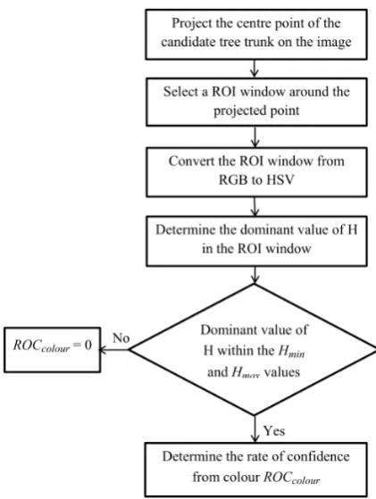
Figure 8 illustrates the procedure for tree trunk colour detection from images. The algorithm determines the most dominant value of the H dimension in ROI selected in the centre of the candidate tree trunk. This value is compared with the H reference values (Hmin, Hmax) to

determine the rate of confidence of the tree trunk colour (ROCcolour).

Tree Trunk Edge Detection

Tree trunk edges are the other features used in this study to detect the tree trunk from images. The Pstart and Pend of the candidate tree trunk detected by the laser

Figure 8: Tree trunk colour detection.

possible straight edge in each window using least-squares linear regression method. This is achieved by fitting a linear model to the edge data in each ROI and calculate the slopem, the angleθand the measure of the goodness of the fitted line R2_{. The rate of confidence from edge}

detection for each tree trunkROCedgesis the summation

of the rate of confidence of the left and the right edges and the degree of the two edges being parallel. Figure 9 explains the procedure for tree edge detection.

5

Map Construction

Map construction process is achieved by moving the mo-bile robot with its onboard camera-laser combination from a known starting position in the midway between two tree rows in equal steps. The image-laser scan pair is acquired at each step to implement tree trunk detection and mapping algorithm.

The mapping algorithm determines the position of the trees and the non-tree objects in the environment using the ranges and bearing angles between the trees and the mobile robot acquired by the laser scanner as shown in Figure 10. The tree trunk coordinates (Xtree, Ytree) for

each tree at each image-scan are determined as follows:

Xtree=Xrobot+rsin(β) (11)

Ytree=Yrobot+rcos(β) (12)

Figure 9: Tree trunk edges detection.

Figure 10: Graphical representation of the trees in the orchard environment.

where r and β are the range and the bearing an-gle between the tree trunk and the mobile robot. Xrobot and Yrobot represent the mobile robot

Figure 11. To map a real orchard, the mobile robot po-sitioning would involve other external and sensory input (data from global positioning (GPS), inertial measure-ment unit (IMU), odometry, etc.).

The final map consists of the coordinates of each tree and non-tree object in the environment. The final po-sition for each individual tree (Xmean, Ymean) is

deter-mined by calculating the mean of Xtree and Ytree for

all the scans of the same tree. Furthermore, the mean of ROCtree for all the scans of each tree is calculated

(ROCtree mean) and added to the final map. The same

procedure is used to determine the position of the non-tree objects.

6

Experimental Results and Discussion

Two experiments have been conducted. The first experi-ment tested the tree trunk detection in a simulated envi-ronment and implemented mapping of this envienvi-ronment. The second experiment tested the tree trunk detection in a natural setting comparable to an orchard.

6.1

Simulated Environment Test for Tree

Detection and Mapping

The camera-laser combination was moved in the simu-lated environment from a known starting position in the midway between two rows in equal steps with respect to the starting position and the image-laser scan pair was acquired at each step. For each image-laser scan pair, the tree trunk detection and mapping algorithm was im-plemented. Figure 3 shows the simulated trees with the selected ROI around the edges.

Four objects were inserted in the simulated environ-ment at different locations between the rows and outside the rows to test the tree trunk detection algorithm. The objects were additional mailing tubes that were modified to be either different in geometry or different in colour. Three of these objects (B1,B3, and B4) had width of

170mm. The fourth object (B2) had the same

dimen-sions of the simulated tree trunks but with a different colour.

Figure 11 shows the final map of the simulated envi-ronment which contains the simulated tree trunks (T1

-T12) and the non-tree objects (B1-B4). Each tree trunk

in this map is represented by green circle with its num-ber, while each non-tree object is represented by red cir-cle with its number.

The standard errors of the tree trunks coordinates (SEx, SEy) were calculated using the following

equa-tion:

SE =√s

N (13)

where s is the data standard deviation andN is the number of image-scan pair for each tree.

Figure 11: The map of the simulated environment.

Table 1 shows the results of each individual tree de-picted in Figure 11. From the results, it can be seen that the range of the ROCtree mean for the simulated

trees was between 0.786 to 0.903 which is acceptable for identifying the tree trunks. There is small variation in SExandSEy results for the simulated trees in Table 1.

This variation is due to the range measurement errors since the laser scanner used in this test has range accu-racy of ±3% of measurement for the range from 20mm to 4000mm [Hokuyo, 2009]. The angular resolution of the laser scanner 0.36◦ also affects the standard error because the number of laser point data decreases with the range for the same object. This affects the bearing angle measurements and errors inSExandSEy.

Table 1: Simulated environment test results for the sim-ulated trees.

Tree N ROCtree mean SEx(mm) SEy(mm)

T1 5 0.903 6.40 8.33

T2 5 0.888 6.09 9.76

T3 6 0.867 3.32 7.54

T4 8 0.890 5.77 8.57

T5 6 0.883 8.20 9.91

T6 8 0.854 8.55 8.17

T7 7 0.885 5.03 7.09

T8 6 0.875 4.31 7.90

T9 6 0.860 3.72 3.75

T10 6 0.877 4.31 7.90

T11 5 0.786 8.18 5.08

T12 5 0.878 8.70 2.85

low ROCtree mean because they have different width

than the simulated trees. The algorithm was capable of distinguishing them from the laser scanner data by determining their width and ROClaser. These objects

hadROClaser less than theROCthand were considered

as non-tree objects. TheROCtree meanofB2was higher

than the other objects sinceB2 had the same width as

the simulated trees but different colour. This object was detected by the laser scanner as candidate tree trunk and the colour of this object was compared with the range of the simulated tree trunk colour. The algorithm detected it as non-tree object because its colour is not within the simulated tree trunk colour range.

Table 2: Simulated environment results for non-tree ob-jects.

Non-tree N ROCtree mean SEx(mm) SEy(mm)

object

B1 5 0.0009 2.95 5.41

B2 5 0.461 3.40 5.66

B3 5 0.0012 5.63 4.21

B4 5 0.0008 5.51 5.91

6.2

Real Tree Test for Tree Detection

Outdoor tests were conducted to test the performance of the vision-based tree trunk detection algorithm in dif-ferent illumination conditions for 20 trees of the same type. The mean of the width of the tree trunk for the 20 trees was 230.15mm with standard deviation of 20.45mm. Three tests were performed that used colour detection, edge detection, and both colour and edge de-tection together.

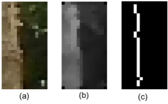
Figure 12(a) demonstrates the projected point in the centre of the tree trunk and the ROI selected around this point, while Figure 12(b) shows the projected points and the selected ROI around each tree trunk edge. Figure 13 shows the RGB colour image, gray scale image and the edge detection image for a selected ROI around a tree trunk edge.

For tree trunk colour detection test, the computed nor-malised values ofHmin andHmax were 0.049 and 0.124

respectively. The average of ROCcolour for all the 20

trees was 0.9, while the average of ROCedges for the 20

trees was 0.705. Therefore, the colour was given more weight than the edges in determining the rate of confi-dence from vision. The average of the rate of conficonfi-dence from both colour and edges detection for the same 20 trees was 0.822.

The tree trunk detection algorithm was also tested for different non-tree objects that might be found in orchard such as bushes and posts. The algorithm assigned a low rate of confidence for them and considered them as ob-jects. Some posts were considered as non-tree objects by the laser scanner because they have different width

com-pared with tree trunk. Other posts were first detected as candidate tree trunk from the laser data because their width is within the range of tree trunk width, however their colour was tested and were considered as non-tree objects because they have different colour compared with tree trunk colour. Furthermore, different types of bushes with different widths were tested. The algorithm was ca-pable of distinguishing some of these bushes as non-tree objects because they have different width compared with tree trunk, while other bushes were first detected as can-didate tree trunk from the laser scanner and then con-sidered as non-tree objects because they have different colour compared with tree trunk colour range.

In this study, a simple heuristic setting of thresholds was appropriate to conduct the preliminary sensor fusion evaluation reported. It is expected that in general or-chard application the thresholding may need to be both variable (i.e. need initial calibration) and also adaptive during operation.

(a) (b)

Figure 12: (a) ROI around tree trunk centre. (b) ROI around tree trunk edges.

Figure 13: (a) RGB image of the ROI around an tree trunk edge. (b) Gray-scale image of the ROI. (c) Edge detection image of the ROI.

7

Conclusion and Future Work

show that the developed algorithm provides sufficient re-sults for tree trunk detection, tree position and orchard mapping. The proposed method of utilising both laser scanner and camera data enhanced the tree trunk de-tection. Projection from the laser scanner to the image plane and selecting the ROI with the required features was effective since it reduced the processing time and minimised the effect of noise in other parts of the im-age. Future work will include developing this method for mapping a real orchard and using the map for local-isation and navigation of mobile robot in the orchard.

Acknowledgments

This work has been supported by the University of Southern Queensland. The senior author would like to acknowledge the University of Technology, Baghdad, Iraq for funding the PhD scholarship.

References

[Ayalaet al., 2008] Marcos Ayala, Carlos Soria, and Ri-cardo Carelli. Visual servo control of a mobile robot in agriculture environments. Mechanics Based Design of Structures and Machines, 36(4):392–410, November 2008.

[Bouguet, 2009]

Jean Bouguet. Camera calibration toolbox for matlab. http://www.vision.caltech.edu/bouguetj/calib doc/.

[Canny, 1986] John Canny. A computational approach to edge detection. IEEE Transactions on Pat-tern Analysis and Machine Intelligence, 8(6):679–698, November 1986.

[Cheeinet al., 2011] F. Cheein, G. Steiner, G. Paina, and R. Carelli. Optimized EIF-SLAM algorithm for precision agriculture mapping based on stems de-tection. Computer and Electronics in Agriculture, 78(2):195–207, September 2011.

[Dreamstime, 2013] Retrieved from http://www.dreamstime.com/stock-photography-apple-orchard-bloom-image14017522.

[Gaoet al., 2010] Feng Gao, Yi Xun, Jiayi Wu, and Guanjun Bao. Navigation line detection based on robotic vision in natural vegetation-embraced environ-ment. In2010 3rd International Congress on Image and Signal Processing (CISP 2010), Yantai , October 2010.

[Guivantet al., 2002] Jose Guivant, Favio Masson, and Eduardo Nebot. Simultaneous localization and map building using natural features and absolute informa-tion. Robotics and Autonomous Systems, 40(2-3):79– 90, August 2002.

[Hamneret al., 2010] Bradley Hamner, Sanjiv Singh, and Marcel Bergerman. Improving orchard efficiency

with autonomous utility vehicles. In2010 ASABE An-nual International Meeting, Pittsburgh, Pennsylvania, June 2010.

[Hansenet al., 2011] Soren Hansen, Enis Bayramoglu, Jens Andersen, Ole Ravn, Nils Andersen, and Niels Poulsen. Orchard navigation using derivative free Kalman filtering. In 2011 American Control Confer-ence, San Francisco, CA, USA, 29 June- 01 July 2011.

[Hokuyo, 2009] Hokuyo Automatic Co. Ltd. Scanning laser range finder URG-04LX-UG01 (Simple-URG)-Specifications, August 2009.

[Kassir and Peynot, 2010] Abdulla Kassir and Thierry Peynot. Reliable automatic camera-laser calibration. In Proceedings of the 2010 Australian Conference on Robotics and Automation (ACRA), Brisbane, Aus-tralia, December 2010.

[Libby and Kantor, 2011] Jacqueline Libby and George Kantor. Deployment of a point and line feature local-ization system for an outdoor agriculture vehicle. In 2011 IEEE International Conference on Robotics and Automation, Shanghai, China, May 2011.

[Meng et al., 2010] Lixia Meng, Fuchun Sun, and Shuzhi Ge. Extrinsic calibration of a camera with dual 2D laser range sensors for a mobile robot. In 2010 IEEE International Symposium on Intelligent Con-trol, Yokohama, Japan, September 2010.

[Peynot and Kassir, 2010] Thierry Peynot and Abdal-lah Kassir. Laser-camera data discrepancies and re-liable perception in outdoor robotics. In the 2010 IEEE/RSJ International Conference on Intelligent Robots and Systems, Taipei, Taiwan, October 2010.

[Rosell Poloet al., 2009] Joan Rosell Polo, Ricardo Sanz, Jordi Llorens, Jaume Arno, Alexandre Escola, Manel Ribes-Dasi, Joan Masip, Ferran Camp, Fe-lip Gracia, Francesc Solanelles, Tomas Palleja, Luis Val, Santiago Planas, Emilio Gil, and Jordi Palacin. A tractor-mounted scanning LIDAR for the non-destructive measurement of vegetative volume and surface area of tree-row plantations: a comparision with conventional destructive measurements. Biosys-tems Engineering, 102(2):128–134, February 2009.

[Subramanianet al., 2006] Vijay Subramanian, Thomas Burks, and A. Arroyo. Development of machine vision and laser radar based autonomous vehicle guidance systems for citrus grove navigation. Computers and Electronics in Agriculture, 53(2):130–143, September 2006.

[Torres-Sospedra and Nebot, 2011] Joaquin