Lateral earth pressure problems involved with cantilever retaining structures and stability of those structures

(1)

University of Southern Queensland

Faculty of Engineering and Surveying

Lateral Earth Pressure Problems involved with

Cantilever Retaining Structures and Stability of those

Structures

Presented By

Mr Scott Clayton

In fulfilment of the requirements of

Bachelor of Engineering

(2)

ABSTRACT

Retaining walls provide support for vertical or near vertical grade changes, while also preventing erosion or down slope movement. The backfill is usually associated with an amount of surface strip load, thereby creating lateral pressure which acts onto the non yielding retaining wall. The purpose of this thesis is to calculate mathematically and graphically the lateral earth pressures and how stability of a retaining structure is influenced by these pressures. Calculations are made which will involve Rankine earth pressure theory and Coulomb earth pressure theory. It also involves determining whether there are any correlations between the two theories. Either Rankine’s or Coulomb’s theory is then taken further to investigate the bearing, sliding and overturning with various soil foundation and backfill material. One of these theories will be representing 64 cases, all unique and presenting varying geometries and soil materials, while backfill is considered inclined throughout. From this outline, the factor of safeties is determined in order to identify the most effective scenario.

(3)

LIMITATIONS OF USE

The Council of the University of Southern Queensland, its Faculty of Health, Engineering & Sciences, and the staff of the University of Southern Queensland, do not accept any responsibility for the truth, accuracy or completeness of material contained within or associated with this dissertation.

(4)

CERTIFICATION OF DISSERTATION

I certify that the ideas, designs and experimental work, results, analyses and conclusions set out in this dissertation are entirely my own eﬀort, except where otherwise indicated and acknowledged.

I further certify that the work is original and has not been previously submitted for assessment in any other course or institution, except where speciﬁcally stated.

(5)

ACKNOWLEDGEMENTS

(6)

Table of Contents

Lateral Earth Pressures

ABSTRACT ... i

CERTIFICATION OF DISSERTATION ... iii

ACKNOWLEDGEMENTS ... iv

LIST OF FIGURES ... vii

LIST OF TABLES ... xii

NOTATIONS ... xiii

ABBREVIATIONS ... xvi

1. INTRODUCTION ... 1

1.1 Risk Assessment ... 1

1.2 Terminology ... 3

1.3 Historical Background ... 4

1.3.1 Coulomb ... 4

1.3.2 Rankine ... 4

2. LATERAL EARTH PRESSURES ... 6

2.1 At-Rest Earth Pressure ... 6

2.2 Rankine Earth Pressures Theory ... 9

2.2.1 Active earth pressure ... 11

2.2.2 Passive earth pressure ... 15

2.3 Coulomb Earth Pressure Theory ... 18

2.3.1 Active earth ... 19

2.3.2 Passive earth pressure ... 22

3. LIMIT ANALYSIS ... 25

3.1 Two-Dimensional Stress ... 26

3.2 Lower Bound ... 28

3.3 Upper Bound ... 31

3.3.1 Passive case ... 32

3.3.2 Active case ... 40

4. ANALYSE OF CANTILEVER WALL ... 50

4.1 Properties ... 50

(7)

4.3.2 Check for Overturning ... 53

4.3.3 Check for Bearing Capacity Failure ... 54

4.3.4 Check for Sliding along Base ... 55

4.3.5 Applied Forces ... 55

5. APPROACHES TO IMPROVE STABILITY ... 73

5.1. Nails ... 73

5.2. Freezing ... 74

5.2.1 Brine Freezing ... 75

5.2.2 Liquid Nitrogen Freezing ... 75

6. OPTUMG2 ... 76

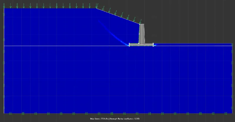
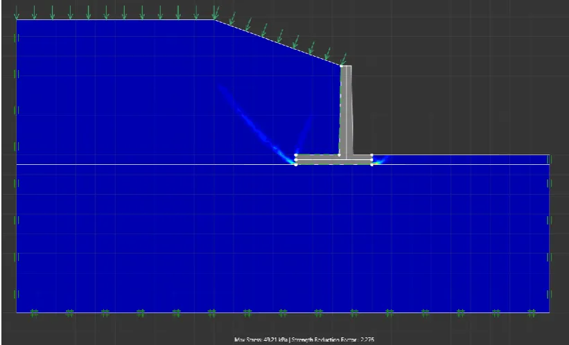
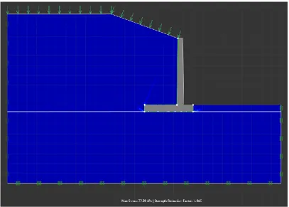
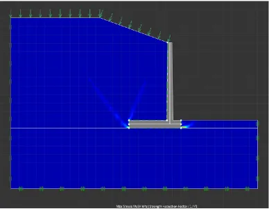
6.1 Strength reduction ... 76

6.2 Lower and Upper Bound Calculations ... 80

6.3 Elastoplastic Analysis ... 85

7. CONCLUSION ... 87

8. REFERENCES ... 89

9. APPENDIX A – Project Specification ... 92

10. APPENDIX B – Acting Forces ... 93

11. APPENDIX C – Soil Properties ... 98

12. APPENDIX D – Rankine Values of for Horizontal backfill ... 99

13. APPENDIX E – Rankine Active Values of for inclined backfill ... 100

14. APPENDIX F – Rankine Passive Values of for inclined backfill ... 102

15. APPENDIX G – Coulomb Active Values of for horizontal backfill , ... 104

16. APPENDIX H – Coulomb Passive Values of for horizontal backfill , . 105

17. APPENDIX I – Coulomb Active Values of for inclined backfill ... 106

18. APPENDIX J – Coulomb Passive Values of for inclined backfill ... 108

(8)

LIST OF FIGURES

Figure 1- Cantilever retaining wall terminology (Denson, 2013) ... 3

Figure 2 - Lateral strain and lateral pressure coefficient (Craig, 2004) ... 7

Figure 3 - Mohr Circle (Craig, 2004) ... 9

Figure 4 - Failure Plans: active case (Craig, 2004) ... 10

Figure 5 – Slip lines for Active and Passive States (Craig 2004) ... 10

Figure 6 – Rotational, Translational Retaining Wall Active Case (Sherif, et al., 1984)... 11

Figure 7 - Active and passive states ... 12

Figure 8 - Earth pressure distribution, cohesive backfill (Braja, 2014) ... 14

Figure 9 – Rotational, Translational Retaining Wall Passive Case (Sherif, et al., 1984) ... 15

Figure 10 - Curvature due to wall friction (Craig, 2004) ... 18

Figure 11 - Coulombs active theory (Valsson, 2011) ... 19

Figure 12 - Coulomb active theory with c > 0 (Craig, 2004) ... 21

Figure 13 - Coulombs passive case (Valsson, 2011) ... 22

Figure 14 - upper and lower bound (HKU, 2013) ... 25

Figure 15 - Shear and normal stresses acting on element ... 26

Figure 16 - Free body diagram CED ... 26

Figure 17 - two dimensional stress state (Davis & Selvadurai, 2005) ... 28

Figure 18 - Discontinuous stress field for vertical cut ... 29

Figure 19 - Mohr diagram for region 1 ... 30

Figure 20 - Wall velocity ... 31

Figure 21 - Passive force triangle ... 32

Figure 22 - Active force triangle ... 40

Figure 23 - Dimensions for given wall ... 50

Figure 24 - Actions ... 50

Figure 25 - Effective width (Braja, 2014) ... 60

Figure 26 - Bearing FoS rock foundation ... 67

Figure 27 - Bearing FoS sand foundation ... 67

Figure 28 - Bearing FoS gravel foundation ... 67

Figure 29 - Bearing FoS Clay/Cl. Silt foundation ... 68

Figure 30 - Sliding FoS Blasted Rock foundation ... 69

Figure 31 - Sliding FoS Sand foundation ... 69

Figure 32 - Sliding FoS Gravel foundation ... 69

Figure 33 - Sliding FoS Clay/Cl. Silt foundation ... 70

Figure 34 - Overturning FoS for blasted rock foundation ... 71

Figure 35 - Overturning FoS for sand foundation ... 71

Figure 36 - Overturning FoS for gravel foundation ... 71

Figure 37 - Overturning FoS for clay/cl silt foundation ... 72

Figure 38 - soil nailing overview... 73

Figure 39 - Ground freezing (Kiger, 2013) ... 74

Figure 40 - 7.5 metre stem wall ... 77

Figure 41 - 1000 elements ... 78

Figure 42 - 2000 elements ... 78

(9)

Figure 44 - Subdivided 7.5 metre stem wall ... 79

Figure 45 - 1000 elements with subdivision ... 79

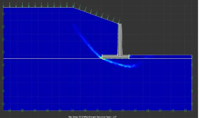
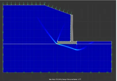
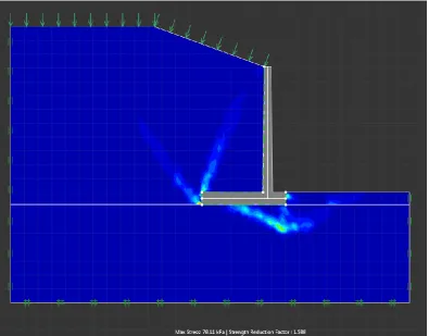
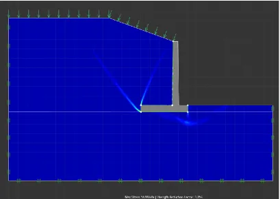
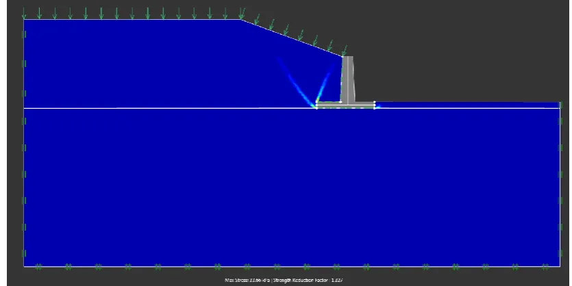
Figure 48 – Blasted rock foundation using OptumG2 ... 83

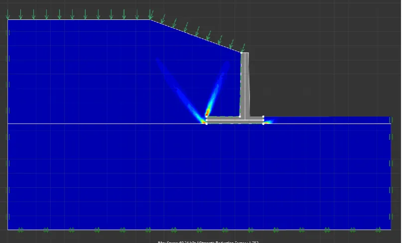
Figure 49 - gravel foundation using OptumG2 ... 83

Figure 50 – Clay/Cl silt foundation using OptumG2 ... 84

Figure 51 – Sand foundation using OptumG2 ... 84

Figure 52 - Total displacement ... 85

Figure 53 - Long term displacement with the use of internal mesh ... 85

Figure 54 - Long term displacement without the use of internal mesh ... 86

Figure 55 - Long term displacement with 100 000 elements ... 86

Figure 0.1 - Lower bound failure mode for case 1 ... 110

Figure 0.2 - Upper bound failure mode for case 1 ... 110

(10)

(11)

(12)

(13)

LIST OF TABLES

Table 1 – Rankine coefficients ... 23

Table 2 – Coulomb coefficients ... 23

Table 3 – Bearing capacity factors (Braja, 2014) ... 54

Table 4 – Wall properties ... 56

Table 5 – Factor of Safety for bearing, sliding, and overturning ... 64

Table 6 – Strength reduction factor with and without subdivisions ... 77

Table 7 – Strength reduction factor with and without mesh adaptivity ... 80

(14)

NOTATIONS

width of the base slab

(15)

sum of the moments of forces acting on the retaining wall

passive force

sum of all the hori ontal forces acting on the wall sum of all the vertical forces acting on the wall

(16)

actual soil density after construction completion

loosest soil density

(17)

ABBREVIATIONS

OCR – Overconsolidated Ratio

FoS – Factor of Safety

SFoS – Strength Based Factor of Safety

ULS – Ultimate Limit State

GEO – Failure of the Ground

LB – Lower Bound

UB – Upper Bound

ULS – Ultimate Limit State

GFRP – Glass Fiber Reinforced Plastic

(18)

1.

INTRODUCTION

A retaining wall is a structure constructed to primarily hold back masses of soil known as backfill (horizontal or inclined). They provide support for vertical or near vertical grade changes, while also preventing erosion or down slope movement. The backfill is usually associated with an amount of surface strip load, thereby creating lateral pressure which acts onto the non-yielding retaining wall. Typical surface strip loads may include highways, building infrastructure, or railroads.

Surface strip loads will become in particular interest in the thesis, especially under circumstances where a rigid retaining wall is directly under its influence. The purpose of this thesis is to calculate mathematically and graphically the lateral earth pressures and how stability of a retaining structure is influenced by these pressures. The selected retaining wall which will be focused upon in this thesis includes the cantilever type structure.

Calculations will be made which will involve Rankine earth pressure theory and Coulomb earth pressure theory. It will also involve determining whether there are any correlations between these two theories. It is known that Rankine’s theory considers the back of the retaining wall as frictionless, while Coulomb considers there to be friction between the retaining wall and backfill.

A numerical approach will involve software known as OptumG2 to determine the representation of the stresses experienced by the retaining wall and the influence it has on the backfill and foundations.

1.1 Risk Assessment

(19)

Hazards

Wherever there is a hazard there is an associated risk factor, if the hazard is unavoidable then the risk may be minimised. In the office environment hazards are seen to be less significant then out in the manufacturing station, however, all types of hazards have the potential to cause serious consequences if not

thoroughly analysed. A list of hazards and their associated risks have been identified below for an office work environment, they include:

 Poor posture – results from repetition of daily activities, can increase stress and strain. Can be caused by excessive duration in a seated position and/or incorrect setup of workstation. This risk is substantial; to reduce this risk regular exercise must be undertaken to stretch muscles. Three prime symptoms listed below which are caused by poor posture.

 Stiff neck  Stiff shoulders  Back pain

 Eye strain – Results from extended use of the eyes, such as excessive computer use and/or poor lighting. This risk is significant, however symptoms are only short term (i.e. headaches and/or blurred vision), hence, will not cause eye damage.

 Glare – Results from direct light source which reflects light from the monitor. This hazard results in eye strain and fatigue. If the hazard is not removed then the risk is substantial. To remove the hazard blinds will need to be closed, clean monitor, or place screen at right angles to the light source.

 Carpal tunnel syndrome – Results from repetitive keyboard use which requires hand movements. The risk is very slight, however carpal tunnel syndrome tend to affect some individuals more than others. The symptoms include numbness, pins and needles, hand weakness, sore wrists, etc.

(20)

1.2 Terminology

For simplicity, Figure 1 details a cross section of a cantilever retaining structure with common terminology and their typical locations.

The stem acts as a cantilever beams, it is imperative that it resist all lateral pressures caused by the soil which acts against it.

The base slab (footing), is structurally designed to withstand vertical pressures, therefore must transmit those pressures to the undisturbed soils.

The key is to resist lateral pressure and movement; it is an optional component within the design of the wall. Location of the key may be located anywhere along the base slab.

Backfill is soil material which is supported by the stem of the retaining wall. Backfill is usually associated with ‘disturbed’ soil material, and elevated to design level.

Figure 1- Cantilever retaining wall terminology (Denson, 2013)

Toe Heel

Front Face

(21)

The back face is the side of the stem which is in contact with the backfill for majority of the retaining walls height. The front face is the side of the stem which is exposed for majority of the retaining walls height.

The toe is the face of the base slab at the front side of the wall, while the heel is the face of the base slab on the back side of the wall.

Drainage is located within the backfill between the stem and the footing of the retaining wall; it is a method in reducing the amount of concentrated water within the backfill. If the drainage system fails then the water won’t dissipate, this will lead to an additional lateral pressure which will act against the wall (Donkada & Menon 2012, para. 3).

1.3 Historical Background

The development of the cantilever retaining wall was induced after the Second World War, following techniques which involved reinforced concrete structures. These walls are designed to cantilever loads to the footing. In order to improve their stability against high loads the wall is usually installed with a counterfort on the back or the wall is buttressed on the footing. However, the theory behind cantilever was introduced by Galileo in the 16th century. Further study within this field continued within the 19th century by John Fowler and Benjamin Baker. In the 1880s the use of reinforced retaining walls were introduced (UMR, 2014).

1.3.1 Coulomb

The first significant contribution to the study of soil behaviour is dated back to 1776 when a French-physicist by the name of Charles-Augustin de Coulomb (1736 – 1806) published an article on wedge theory of earth pressure. It was Coulomb that introduced the concept that shear resistance of soil is made up of two components, i.e. cohesion and friction (Shroff & Shah 2003).

1.3.2 Rankine

(22)

(23)

2.

LATERAL EARTH PRESSURES

Lateral stress values involved in retaining structures depend primarily on the

geometry of deformation. In detail, the lateral earth pressure depends on two factors, the stem of the retaining wall and the supported material. Earth pressure will vary accordingly to both magnitude and direction of the retaining wall stem, while also considering the cohesive strength and the internal friction of the supported material. The pressure distribution is typically triangular in shape, increasing the further the depth.

All soil materials are associated with a certain mass, more or less than others, and as a result all soil masses have internal stresses. However, the magnitudes of these stresses are directly influence by the properties of the surrounding geometry, quantity of soil material and any external loadings. A retaining wall must be structurally designed so the stresses applied by the soil mass are counteracted. In order for this, the retaining wall must provide a pressure equal and opposite to the pressures applied by the soil.

Rankine and Coulomb are based on five fundamental assumptions, they require:  the backfill soil to be granular and cohesionless; it must contain very little or

no fine grained soil particles (i.e. silt and clay);

 the soil is homogenous (i.e. contains no mixture of materials);

 the soil is isotropic, (i.e. equal stress-strain properties in all directions and no artificial reinforcement);

 no boundary conditions, that is, the wall and soil are considered semi-infinite and soil left undisturbed;

 drained soil conditions, so pore water pressure can be ignored.

2.1 At-Rest Earth Pressure

If the wall is static then the soil adjacent becomes in a state of static equilibrium (Braja & Khaled, 2014). In this case, in order to define the earth pressure coefficient, , with soil having a unit weight of at depth z:

(24)

Where:

Craig (2004) refers in his report that since the soil which experiences at-rest condition does not fail, then the horizontal and vertical stresses represented within the Mohr circle does not touch the failure envelope and the hori ontal stress can’t be mathematically calculated. Therefore, experimental procedures must be used. Figure 2 details the form of relationship between lateral pressure coefficient and lateral strain.

Alternatively, Jaky (1944) has represented a formula which is widely accepted for the normally consolidated soils, the coefficient of earth pressure at rest can be estimated by:

(25)

_{Eq. 2.2}

Where:

Eq. (2.2) is applicable only for calculations involving loose deposits (e.g. non-compacted sands), where only compaction is by gravity. However, when the soil becomes densified Eq. (2.2) does not represent accurate results (Sherif, Fang and Sherif 1984), as it induces additional horizontal stresses acting against the wall which is not considered within the given formula. This has been experimentally conducted by Sherif, Fang, and Sherif. Due to this predicament, a formula which resolves only around densified soil types has been recommended:

Eq. 2.3

Where:

actual soil density after construction completion

loosest soil density

Braja & Khaled remarks on the increase in the earth pressure coefficient between Eq. (2.2) and Eq. (2.3), due to over consolidation. Therefore, calculations

involving over consolidation must be considered in order to minimise this difference between both formulas.

Hanna & Al-Romhein stated the significants of Wroth, Meyerhof and Mayne and Kulhawy’s contribution, involving experiments which resulted in their

recommendation of Eq. (2.4), which is a modification of Eq. (2.2). A quote from Wroth, Meyerhof and Mayne and Kulhawy’s states ‘formula provided good agreement with the experimental results of the coefficient of earth pressure at rest

(26)

Eq. 2.4 Where;

2.2 Rankine Earth Pressures Theory

Rankine’s theory involves the consideration of the stress levels in the soil when the plastic equilibrium has been reached (Braja & Khaled, 2014). Rankine’s method in distinguishing the stress levels at failure is represented by Mohr circle, this is achieved in a two dimensional plane, detailed in Figure 3.

Where are the relevant shear strength parameters.

Using the failure envelope given in the Mohr circle and substituting the horizontal and vertical stresses for the minor and major principle stresses, Rankine was able to determine equations which calculated the active and passive pressure

coefficients.

Shear failure occurs along a plane at an angle of to the major principle plane. Theoretically, if a mass of soil is stressed that the principle stresses are in the same direction at every point, then there will be a network of failure planes. This is detailed in Figure 4.

(27)

Now, let’s to consider a semi-infinite mass of soil being restrained by a frictionless wall of semi-infinite depth between points AB, this is detailed in Figure 5. The soil is considered to be homogenous and isotropic. The relationship between active and passive soil conditions can be determined through the

inclinations of the slip line; also detailed in Figure 5. Craig (2004) declares that when the horizontal stress is equal to the active pressure, then the soil is within the active Rankine state. In the active Rankine state the shear opposes the effect of gravity (Lambe, 1969), where there are two sets of shear lines (failure planes) inclined at an angle of to the horizontal (Craig, 2004).

Craig (2004) also elaborates when the horizontal stress equals the passive pressure, then the soil is in a passive Rankine state. In the passive Rankine state

Figure 4 - Failure Plans: active case (Craig, 2004)

A

B

A

(28)

the shear stress acts together with gravity to oppose the horizontal stress from the inward movement of the wall (Lambe, 1969). Where there are two sets of shear lines (failure planes) inclined at an angle of to the vertical (Craig, 2004).

Therefore, the two different pressure cases include:  active pressure; and

 passive pressure.

Craig (2004) refers to these two pressures as limit pressures; this will be discussed in more detail within section 2.2.1 and section 2.2.2.

2.2.1 Active earth pressure

Cohesionless Soils,

A retaining wall can undergo several types of movements which can possibly lead to failure due to active pressure; these types of movements are detailed in Figure 6.

2.2.2 2.2.3 2.2.4 2.2.5 2.2.6 2.2.7 2.2.8 2.2.9

If the wall is allowed to move away from the backfill, such to represent an active case, then the overall lateral principle stress will decrease (Braja & Khaled, 2014). Therefore, active case represents a minimal value since the

(29)

soil can laterally expand as the wall moves outwards. When the soil expansion is large enough, then the minimum value of is achieved, leading to a state of plastic equilibrium (White, 2011). Since the horizontal stress is the cause of this development, then must be the minor principle stress, (Craig, 2004). Therefore the major principle stress is the vertical stress, .

The relationship between the major and minor principle stresses when the soil reaches a plastic equilibrium state can be determined through the Mohr circle.

Now, if the wall undergoes a rotational movement about the toe, detailed in Figure 6a, the horizontal stress at any depth would not alter, . Figure 7 details the stress condition in the soil represented by the Mohr’s circle ‘state of rest’. However, for an active case the horizontal principle stress detailed in Eq. (2.5) would decrease (i.e. . This state of stress is represented by the Mohr’s circle ‘active Rankine state’.

Eq. 2.5

Where;

Figure 7 - Active and passive states Failure Envelope

State of Rest

(30)

; and

If the active earth pressure coefficient is defined as , then equation 2.5 is rewritten:

_{Eq. 2.6}

Active Rankine state occurs when the horizontal stress is equal to the active pressure.

Where;

Eq. 2.7 Values of Rankine’s active pressure coefficients (Eq. 2.7) for various values of are detailed in Appendix D.

Inclined Backfill

In a case where the backfill contained behind a frictionless retaining wall is a granular type soil and the angle is inclined to the horizontal at which the soil rises , then the active earth pressure coefficient, can be

determined:

Eq. 2.8

Where;

This data from Eq. 2.8 for various values of has been represented and detailed in Appendix E.

From this collection of data the Rankine active pressure at any depth can be determined:

_{Eq. 2.9}

And;

(31)

_{Eq. 2.10}

Cohesive Soils

For a frictionless retaining wall with cohesive soil backfill, at any depth the active soil pressure against the wall can be determined:

It is detailed in Figure 8a the variation of with depth, and detailed in Figure 8b the variation of with depth.

Therefore, overtime, tensile cracks will develop at the soil-wall interface up to a total depth (Braja & Khaled, 2014). The area of the total pressure diagram in Figure 8c can be used to calculate the total active force per unit length of wall. For calculation of the total active force with a horizontal cohesive backfill,

_{Eq. 2.11}

It was detailed by Braja that for active earth pressures for clayey soils is equated differently to that of soft soils. The formula denoted below can be compared to that of Eq. 2.13.

(32)

Eq. 2.12

; and

For soft soils, . Therefore:

_{Eq. 2.13}

Inclined Backfill

For a cohesive backfill, the active pressure at any depth is determined:

_{Eq. 2.14}

2.2.2 Passive earth pressure

Cohesionless Soils,

A retaining wall can undergo several types of movements which can possibly lead to failure due to passive pressure, they are:

 rotational about the toe;  rotational about the top; and  translational as a rigid body.

These types of movements are detailed in Figure 9.

(33)

If the wall is allowed to move towards the backfill, such to represent a passive case, then the overall lateral principle stress will increase due to compression (Braja & Khaled, 2014). Therefore, passive case represents a maximum value since the soil is laterally compacted as the wall moves inwards. When this maximum value is achieved the limiting compressive strength of the soil is reached (White, 2011).

The relationship between the major and minor principle stresses when the soil reaches a plastic equilibrium state can be determined through the Mohr circle detailed in Figure 7.

Now, if the wall undergoes a rotational movement about the toe, detailed in Figure 9a, the horizontal stress at any depth would not alter, . Figure 9 details the stress condition in the soil represented by the Mohr’s circle ‘state of rest’. However, for a passive case the horizontal principle stress detailed in Eq. (2.5) would increase (i.e. . In this situation the wall will create a state where the soil element will be represented by the Mohr’s circle ‘passive Rankine state’. Failure of the soil will occur at this point in time where the Mohr’s circle touches the failure envelope (Braja & Khaled, 2014). This horizontal principle stress can be determined through the following:

Eq. 2.15 Where;

Eq. 2.16

Therefore, from equation 2.15:

;

_{Eq. 2.17}

The passive force per unit length of wall can be determined:

(34)

Rankine’s passive earth pressure coefficient has been determined in Appendix D for various values of .

Inclined Backfill

The Rankine passive pressure at any depth containing a granular backfill can be determined similar to that of equation 2.15, 2.17 and 2.18. That is;

Rankine passive pressure:

_{Eq. 2.19}

And;

The total passive force per unit length of wall:

_{Eq. 2.20}

The resultant force is inclined at an angle of to the horizontal and intersects the wall at a distance of H/3 from the bottom of the wall. Where;

Eq. 2.21

Rankine’s passive earth pressure coefficient has been determined in Appendix E for various values of and .

Cohesive Soils

At any point, the horizontal effective pressure at any depth, is calculated through the Rankine earth pressure, and is given as:

_{Eq. 2.22}

The force per unit length of the wall is determined:

(35)

Inclined

It was detailed my Braja that for passive earth pressures for cohesive materials such as clayey soils is equated differently to that of non-cohesive materials. The formula denoted below can be compared to that of Eq. 2.23.

_{Eq. 2.24}

2.3 Coulomb Earth Pressure Theory

Rankine’s earth pressure theory involves the assumption that the retaining wall is frictionless. Coulombs method for calculating earth pressure is similar; however friction is taken into consideration. This theory also involves the consideration of the stability of the wedge of soil between the retaining wall and a trial failure plane (Craig, 2004). The forces per unit length of the wall acting on the wedge are determined by calculating the equilibrium of forces acting on the wedge. This calculation is made when the wedge is at the point of sliding up or down the failure plane. The forces include:

 weight of the wedge, W;

 active/passive force, ; and

 resultant force, R, of the normal and shear forces on the failure plane BC

In both active and passive cases the shape of the failure plane is curved near the bottom of the wall due to wall friction, this is detailed in Figure 10. However, in the Coulomb theory the failure plane is assumed to be plane active and passive case.

(36)

2.3.1 Active earth pressure

Figure 11 details a failure wedge ABC, with active forces on the wedge between the wall surface and the failure plane BC. Soil type contains

cohesion parameter c equal to zero. For the failure condition, the soil wedge acting under its own weight (W) is in equilibrium. The reaction force (P) between the wall and soil and the reaction on the failure plane (R). Since the wedge moves down the failure plane BC, then the reaction force P is

declined at an angle to the normal. At failure, the reaction force R along the failure plane is declined at an angle of to the normal. These three forces are then connected head-to-tail (triangle of forces) to determine the magnitude of P. This is detailed in Figure 11.

In this procedure, multiple cases of failure planes will need to be selected to determine the maximum value of P, which would be defined as the

maximum active thrust on the retaining wall (Craig, 2004). However, an alternative method in calculating P would include expressing P in terms of W and the angles , and differentiating with respect to . That is,

:

_{Eq. 2.25}

(37)

Where;

Eq. 2.26

The calculated maximum active thrust is assumed to act at a total distance of H/3 above the base of the retaining wall. Coulomb’s active earth pressure coefficient has been determined in Appendix G for various values of and Appendix I for various values of and .

Now;

Coulombs theory can be associated with soil cohesion c greater than zero. A value is then selected for the wall parameter, . From Figure 12, tension cracks are assumed to extend to a total depth , there the new failure plane extends from the heel of the wall (B) to the bottom of the tension zone (C). The forces acting on the wedge at failure include:

 the weight of the wedge (W);

 the reaction force (P) between the wall and soil declined at an angle to the normal;

 the reaction on the failure place (R) declined at an angle of to the normal;

 The force due to the constant component of shearing resistance on the wall . Where EB is the vertical distance from the base of the wall to the bottom of the tension zone;

 The force on the failure plane due to the constant component of shear strength .

(38)

An alternative method in calculating P would include expressing P in terms of horizontal and vertical forces, and differentiating with respect to . That is, :

A second coefficient is calculated for drained and undrained: undrained conditions:

drained conditions:

In general, active pressure at depth z:

Eq. 2.27

Where;

Eq. 2.28

(39)

The depth of a dry tension crack is:

Eq. 2.29

The depth of a water filled crack is given from the condition:

2.3.2 Passive earth pressure

Figure 13 details the Coulombs passive case; the reaction force P is inclined at an angle to the normal. At failure, the reaction force R along the failure plane is inclined at an angle of to the normal. The overall passive resistance is equal to the minimum value of P, this is given by:

_{Eq. 2.30}

Where;

(40)

Eq. 2.31

The calculated maximum passive thrust is assumed to act at a total distance of H/3 above the base of the retaining wall. Coulomb’s passive earth pressure coefficient has been determined in Appendix H for various values of

Appendix J for various values of and .

In summary Rankine’s theory considers the back of the wall frictionless, while coulomb considers friction between both wall and soil. As a result, when friction angle is equal to zero ( Coulombs formulas are equated equally to that of Rankine’s. Equation 2.8 and 2.21 were used to determine Rankine values detailed in Table 1, while equations 2.26 and 2.31 were used to determine Coulomb values detailed in Table 2. A more detailed outline of Rankine’s coefficients can be found in appendix D, while Coulombs coefficients are further detailed in appendix G and H.

Table 1 - Rankine coefficients Table 2 - Coulomb coefficients

RANKINE

24 0.4217 2.3712

25 0.4059 2.4639

26 0.3905 2.5611

27 0.3755 2.6629

28 0.3610 2.7698

29 0.3470 2.8821

30 0.3333 3.0000

31 0.3201 3.1240

32 0.3073 3.2546

33 0.2948 3.3921

34 0.2827 3.5371

35 0.2710 3.6902

36 0.2596 3.8518

37 0.2486 4.0228

38 0.2379 4.2037

39 0.2275 4.3955

40 0.2174 4.5989

COULOMB,

24 0.4217 2.3712

25 0.4059 2.4639

26 0.3905 2.5611

27 0.3755 2.6629

28 0.3610 2.7698

29 0.3470 2.8821

30 0.3333 3.0000

31 0.3201 3.1240

32 0.3073 3.2546

33 0.2948 3.3921

34 0.2827 3.5371

35 0.2710 3.6902

36 0.2596 3.8518

37 0.2486 4.0228

38 0.2379 4.2037

39 0.2275 4.3955

(41)

In reality designers will find Rankine’s approach to calculating soil pressure a simplified method over Coulombs approach. Rankine’s results gives a lower value than the true value due to a more efficient distribution of stress could possibly exist, this is known as a lower bound solution. In contrast, Coulombs method is more practical for a real life scenario, as this involves friction. Briaud (2013) details that Coulombs solution is a limit equilibrium solution which is greater than the true solution; this is known as an upper bound solution. In this context, Coulombs passive earth pressure coefficient calculates out to be a very large result, possible too large. It was recommended by Craig (2004) that an alternative method be used when

determining Coulombs passive earth pressure coefficient.

(42)

3.

LIMIT ANALYSIS

Limit analysis is a method of approximating limit pressures that provide a lower and upper bound to the true limit load. They are widely used to analyse the stability of geotechnical structures. The upper bound theorem states that collapse must occur if the rate of work due to external forces of the kinematic system in equilibrium equals

or exceeds the rate of dissipated internal energy for all kinematically acceptable

velocity fields (Vrecl & Trauner, 2010). The lower bound theorem states that

collapse will not occur if external loads are in equilibrium with an internal stress field without violating the yield criterion anywhere in the soil mass (Di Santolo, et al., 2012). When both upper and lower bound solution are equal, then the solution is found (HKU,2013), an illustration is detailed in Figure 14.

(43)

3.1 Two-Dimensional Stress

Plane stress is a state of stress where two faces of an element (cubic) are free of stress. Figure 15 depicts a soil element with shear and normal stresses acting.

The conditions for equilibrium of a triangular element detailed in Figure 16 with faces perpendicular to the axes are

It should be noted that the following equations are summarised and for a more detailed outline of equations preformed, refer to Appendix B.

Resolve forces in direction of

(44)

Resolve forces in direction of

Eq. 3.2 The directions of planes on which can be found by substituting in equation 3.2, we get

Eq. 3.3

Equation 3.3 will give two sets of orthogonal planes. This means that there are two planes at right angle to each other on which the shear stress is zero. As a result, since the shear stress is equal to zero on these planes, then these are the planes on which the principal stresses act.

The principal stresses on these planes can be evaluated by substituting equation 3.3 into 3.1, which yields

Two variables of are obtained, the major (larger value, ) and the minor (smaller value, ) of the two principal stresses, this is detailed in Figure 16.

The Major Principal Stress

The Minor Principal Stress

(45)

From Figure 17, the points R and M represents the stress conditions on planes DA and DC. A line RM will intersect the normal stress axis at the center, O. Where OR is the radius of the Mohr cirlce and is equal to:

3.2 Lower Bound

The Lower Bound (LB) solution is identified by calculating the stress under which the soil is in equilibrium. The higher the lower bound solution, the closer it becomes to the exact solution (HKU, 2013).

There are three essential steps for LBs, the first includes the assumption of safe distribution of stress, which must be in equilibrium. The second is the stresses must be less than or equal to the stresses which will cause failure. The last is the use of Mohr circles at different regions to determine the collapse load. It is worthwhile to note that the LB method provides pessimistic answers (Liu, 2010). The advantage of the lower bound solution allows the evaluation of the thrust magnitude, inclination and the point of action (Di Santolo, et al., 2012).

In order to calculate the lower bound solution the stress distribution (equilibrium with the external loads) must not exceed the failure stresses (Di Santolo, et al.,

(46)

2012). With an inclined backfill angle of to the horizontal, a statically admissible stress field which must satisfy all stress boundaries conditions is:

Region 1

The stresses identified in region 1 include:

Since the coordinate origin is located at the top of the cut these stresses will satisfy equilibrium as well as the traction free boundaries, traction free boundary simply means the surface is free from any external stresses. The Mohr circle for region 1 is detailed in Figure 19.

(47)

Region 2

The stress located in the z-component must be continuous across the dashed line, therefore will be given . The stress in the x-component is unidentified at current state.

Region 3

Stress in the x-component from region 2 must remain continuous across the dashed line, and to satisfy the zero traction boundary condition on the surface, therefore (Davis & Selvadurai, 2005). Note for the LB theorem, the stresses everywhere cannot exceed yield point.

Now refer back to Figure 16, the Mohr circle will achieve its greatest diameter when . Therefore, the maximum possible height will occur when the Mohr circle touches the yield envelope. Hence, the critical height is given by

Eq. 3.4

Where;

Let’s refer back to the hori ontal stress, , now in order for the LB theorem to work we must find a stress field that will satisfy equilibrium throughout, while also nowhere exceeding the yield point. This can be achieved by letting;

(48)

in both regions 2 and 3.

An isotropic stress field will be created in region 3, while a Mohr circle for region 2 no greater than that detailed in Figure 19.

Eq. 3.4 represents an equation which can be rearranged, hence let Therefore, Now, let

Hence, the lower bound critical height is

3.3 Upper Bound

The Upper Bound (UB) solution is identified by calculating the stress that causes the soil to fail. The lower the upper bound solution, the closer it becomes to the exact solution (HKU, 2013).

There are two essential steps for UBs, the first includes the determination of

dissipation along interface of velocity jumps using velocity diagrams, a

hodograph has been detailed in Figure 20. The second is the use of energy balance to determine the collapse load. It is

(49)

There are two cases which will be considered throughout the calculations; they include the passive and active cases.

3.3.1 Passive case

In the passive case, the wall moves to the right and the failure wedge moves up and to the right. The force triangle from the hodograph has been constructed and detailed in Figure 21. The wall velocity relative to the stationary mass is . The

other velocities include:

From Figure 20, length (L) of the slip line is determined from the simple sine rule.

The weight of the failure wedge is:

(50)

Thus, the rate of dissipation is:

Eq. 3.5

And, the power of the external forces is:

Eq. 3.6 Where, represents the passive thrust on the wall.

Now, in order to calculate a dimensionless form for the passive thrust, we must equate both 3.5 and 3.6.

To Simplify multiply both the denominator and numerator of the RHS by

(51)

Furthermore Or

Now, let

_AND

Now, to minimise we must adjust and hence find the upper bound for the passive state. When we do this it is found that (critical value) is dependent of .

(52)

Thus, using quotient rule And And

The LHS of (1) simplifies to

(53)

(54)

But

Then

But

And

Then

But

(55)

And

Then

For a blasted rock backfill with ,

But

And

But

(56)

And

Then

But

Then

But

And

Then

Now, let’s consider the RHS

(57)

Now, through the use of iterations, the value for is , for a cohesionless soil, , with , then the passive upper bound estimates to:

3.3.2 Active case

In the active case, the wall moves to the left and the failure wedge moves down and to the left. The force triangle from the

hodograph has been constructed and detailed in Figure 22. The relative velocities include:

From Figure 20, length (L) of the slip line is determined from the simple sine rule.

(58)

The weight of the failure wedge is:

Thus, the rate of dissipation is:

Eq. 3.7

And, the power of the external forces is:

Eq. 3.8 Where, represents the passive thrust on the wall.

Now, in order to calculate a dimensionless form for the passive thrust, we must equate both 3.7 and 3.8.

(59)

To Simplify multiply both the denominator and numerator of the RHS by Furthermore Or

Now, let

_AND

(60)

Hence,

(61)

And

The LHS of (1) simplifies to

But

And

(62)

(63)

But And Then But And Then

Since ,

(64)

But

And

Then

But

And

Then

(65)

Then But And Then Now, let’s consider the RHS

(66)

(67)

4.

ANALYSE OF CANTILEVER WALL

4.1

Properties

Bruner (1983) mentions the design of the stem height in cantilever retaining walls is a function of the difference in required elevation on each side of the stem, and additionally, the depth of cover on the toe side of the stem. Bruner (1983) also elaborates that the design of the footing width is a function of the height of the stem and its stability requirements. The geometrical data is detailed in Figure 24.

Therefore, a stability analysis is undertaken in order to determine the minimum required heel width of a cantilever retaining wall. This minimum width is determined by checking the Ultimate Limit State (ULS), which involves:

 Failure of the Ground (GEO) – This involves the bearing failure of the foundation and the sliding resistance on the base.

(68)

For GEO ULS the failure will occur in the ground, hence the wall movements will be large enough to mobilise the active earth pressures along the virtual back of the wall (Frank, et al., 2004). This pressure is inclined at an angle equal to that of the sloped backfill; this is detailed in Figure 23. It must be noted that the active earth pressure located on the virtual back implies that the width of the heel is large enough to allow the development of a conjugate Coulomb type failure surface located above the heel within the soil mass. This failure surface is inclined at an angle of . Therefore, the width of the heel should not be much smaller, hence a minimum value of:

Eq. 4.1

4.2 Backfill Soil

Course grained, granular soils are known for their high permeability and are therefore the preferred backfill soils. The large void spaces allow quick dissipation of the excess pore water pressure, which brings about a drained condition and reduces the stresses imposed on the retaining wall. However, the outcome will principally depend on cost and availability of such materials. The drained condition only occurs when the water dissipates through the soil, therefore only the soil particles support the loads. Alternatively, the undrained condition only occurs when the water is retained within the soil, therefore the loads are supported by both soil particles and water (White, 2011). Drained or undrained condition primarily depends on the soil type, geological formation, distribution of grain size, artificial drainage systems (installed in backfill), and rate of loading (Budhu, 2007).

(69)

4.3 Stability Check

The Factor of Safety (FoS) has a large influence on the design of a retaining wall. For instance, the international building code (2006) requires a global FoS of 1.5 against overturning and lateral sliding of retaining walls (GuhaRay, et al., 2013).

Various definitions of FoS are used in geotechnical engineering. There are three commonly used FoS listed below:

 factor on material strength;  factor on load; and

 factor defined as ratio of resisting forces to disturbing forces.

As mentioned in paragraph 4.1, a limit state is a state when a structure no longer satisfies the relevant design criteria. For any given design, stability is provided and the design is far from its ultimate limit state. Therefore to undertake an ULS analysis it is required to drive the system till collapse.

In order to drive a system to ULS which correspond to the three FoS definitions list above, include:

 reducing the soil strength;  increasing an existing load; and  place an additional load in the system.

Whenever soil is excavated there is a chance that movement of soil will cause collapse (covered in paragraph 2.2.1 and 2.2.2), this may either be influenced by:

 sliding forward (translational, 2.2.1c.);  bearing capacity failure;

 overturn about its toe (2.2.1a.);

 rotation around a failure plane which encompasses the structure; and  slipping down a inclined slope.

(70)

4.3.1 Tension at Base

The eccentricity, , of the resultant force which acts on the base slab is calculated as

Eq. 4.2

here

width of the base slab

sum of all the vertical forces acting on the wall.

Eccentricity should be less then in order for there to be no tension soil pressure developed at the base. If this condition is satisfied then criterion for overturning is automatically satisfied.

However, if then tension soil pressure will be present at the heel of the base slab, and redistribution of soil pressure takes place to keep it

compressive throughout (Braja, 2014).

4.3.2 Check for Overturning

The FoS against overturning of a wall about its toe is expressed;

Eq. 4.3

(71)

4.3.3 Check for Bearing Capacity Failure

The FoS for bearing of the retaining wall along the base is expressed as

Eq. 4.4

Where, the maximum pressure acting at the base slab of the wall is expressed as and;

The ultimate bearing capacity is expressed as

Where:

are considered shape factors, which are used to determine the bearing capacity of a rectangular footing (Braja & Khaled, 2014).

are considered depth factors, which account for the shearing resistance developed along the failure surface in soil located above the footing (Braja & Khaled, 2014).

are considered inclination factors, which are used to determine the bearing capacity of a footing, where the load application is inclined at a certain angle to the vertical (Braja & Khaled, 2014).

(72)

From table 4, for blasted rock with the bearing capacity factors are

A global FoS required against bearing failure is no less than 3.

4.3.4 Check for Sliding along Base

The FoS for sliding of the retaining wall along the base is expressed as

Eq. 4.5 here

sum of all the hori ontal forces acting on the wall. A global FoS required against sliding is no less than 1.5.

4.3.5 Applied Forces

Determining the total active and passive horizontal forces acting on a cantilever retaining wall will result in determining whether the structure is safe against sliding. Horizontal active forces acting on the virtual back and the horizontal resistance has been identified in Figure 23. It is recognised in this situation that should be treated as a favourable force as to appose (Frank, et al., 2004).

Horizontal active force, Where;

Resistance force,

Where;

(73)

4.4 Scenario: Blasted Rock Backfill AND Blasted Rock Foundation

A surcharge load,

For Active Forces applied on the virtual wall:

(74)

From Appendix G, with variable given in Appendix B and Table 4:

Between wall friction angle

From Equation 4.1:

Where, virtual back, :

For Passive Forces:

From Appendix H, with variable given in Appendix B and Table 4:

Between wall friction angle

From Eq. 3.18 or 3.25, :

20 30 20.0000 0.4142 15.000 0.4150

(75)

Now, ;

Calculating eccentricity, through the overturning moment, ;

(76)

The eccentricity e of the resultant force which acts on the base slab can be determined from Eq. 5.2. If eccentricity is less than or equal to then there will be no tensile pressure developing at the base. If this is the case than the criterion for overturning is satisfied. However, if eccentricity is greater than then tension will be present at the heel of the base slab, and the soil pressure will have redistributed to keep it compressive throughout (Braja, 2014).

(77)

Effective foundation width,

The idea behind the effective width is detailed in Figure 25.

The maximum allowable pressure exerted onto the base slab is given by ;

Now, to determine the factor of safety of the chosen the foundation:

The ultimate bearing capacity is given by:

(78)

Depth Factors

If the value of , then:

However, if the value of , then:

Inclination Factors

Where

(79)

Since

Therefore, from Eq. 5.4 the Factor of safety against bearing capacity failure is:

Therefore, OK.

Now, the FoS of sliding failure can be determined with Eq.5.5:

(80)

Now, the FoS of overturning failure for the chosen strip footing:

(81)

Table 5 – Factor of Safety for bearing, sliding, and overturning Case (m) Bearing Sliding Overturning Backfill material Foundation material

1 2.5 2.92 153.03 56.83 0.21 2.50 75.66 3.96 1.12 5.73 Bl. Rock Bl. Rock

2 5.0 4.25 532.16 205.65 -0.07 4.12 113.71 3.62 1.03 3.77 Bl. Rock Bl. Rock

3 7.5 5.58 1135.94 446.34 -0.36 4.85 124.64 4.78 1.01 3.14 Bl. Rock Bl. Rock

4 10.0 6.90 1965.64 778.93 -0.66 5.58 121.26 6.45 0.99 2.83 Bl. Rock Bl. Rock

5 2.5 2.72 81.58 11.26 0.74 1.25 78.74 6.83 0.15 16.37 Sand Bl. Rock

6 5.0 3.84 300.73 22.59 0.30 3.26 114.23 5.98 0.52 16.60 Sand Bl. Rock

7 7.5 4.97 615.19 33.92 0.28 4.40 166.23 6.25 1.06 18.56 Sand Bl. Rock

8 10.0 6.09 1060.08 98.62 0.13 5.83 196.18 6.69 3.67 9.94 Sand Bl. Rock

9 2.5 2.80 120.98 43.88 0.14 2.52 59.06 5.75 0.55 5.52 Gravel Bl. Rock

10 5.0 3.99 393.92 153.72 -0.17 3.65 73.59 5.80 0.50 3.51 Gravel Bl. Rock

11 7.5 5.19 821.17 329.43 -0.49 4.21 68.66 9.00 0.48 2.88 Gravel Bl. Rock

12 10.0 6.39 1402.72 571.03 -0.81 4.76 51.76 15.68 0.47 2.57 Gravel Bl. Rock

13 2.5 3.05 63.43 11.73 2.47 1.88 121.66 4.35 0.04 20.21 Clay/Cl. Silt Bl. Rock 14 5.0 4.52 334.59 23.55 0.92 2.67 164.98 3.75 0.19 22.58 Clay/Cl. Silt Bl. Rock 15 7.5 5.98 759.72 35.36 0.69 4.61 214.66 4.32 0.43 26.54 Clay/Cl. Silt Bl. Rock 16 10.0 7.45 1338.83 47.18 0.60 6.24 267.23 4.62 0.77 30.88 Clay/Cl. Silt Bl. Rock

17 2.5 2.92 154.27 56.83 0.21 2.50 75.66 6.55 1.12 5.73 Bl. Rock Gravel

18 5.0 4.25 532.16 205.65 -0.07 4.12 113.71 7.46 1.03 3.77 Bl. Rock Gravel

19 7.5 5.58 1135.94 446.34 -0.36 4.85 124.64 8.67 1.01 3.14 Bl. Rock Gravel

20 10.0 6.90 1965.64 778.93 -0.66 5.58 121.26 11.16 0.99 2.83 Bl. Rock Gravel

21 2.5 2.72 81.58 11.26 0.74 1.25 78.74 9.85 0.15 16.37 Sand Gravel

22 5.0 3.84 300.73 22.59