Master equations beyond the Born-Markov approximations
.
White Rose Research Online URL for this paper:
http://eprints.whiterose.ac.uk/121523/
Version: Accepted Version
Article:
Iles-Smith, J, Dijkstra, AG orcid.org/0000-0003-2298-4736, Lambert, N et al. (1 more
author) (2016) Energy transfer in structured and unstructured environments: Master
equations beyond the Born-Markov approximations. The Journal of Chemical Physics, 144
(4). 044110. ISSN 0021-9606
https://doi.org/10.1063/1.4940218
[email protected] https://eprints.whiterose.ac.uk/ Reuse
Unless indicated otherwise, fulltext items are protected by copyright with all rights reserved. The copyright exception in section 29 of the Copyright, Designs and Patents Act 1988 allows the making of a single copy solely for the purpose of non-commercial research or private study within the limits of fair dealing. The publisher or other rights-holder may allow further reproduction and re-use of this version - refer to the White Rose Research Online record for this item. Where records identify the publisher as the copyright holder, users can verify any specific terms of use on the publisher’s website.
Takedown
If you consider content in White Rose Research Online to be in breach of UK law, please notify us by
Energy transfer in structured and unstructured environments: master
equations beyond the Born-Markov approximations
Jake Iles-Smith,1, 2, 3,a)Arend G. Dijkstra,4
Neill Lambert,5
and Ahsan Nazir2,b)
1)Controlled Quantum Dynamics Theory, Imperial College London, London SW7 2PG,
United Kingdom
2)Photon Science Institute & School of Physics and Astronomy, The University of Manchester, Oxford Road,
Manchester M13 9PL, United Kingdom
3)Department of Photonics Engineering, DTU Fotonik, Ørsteds Plads, 2800 Kongens Lyngby,
Denmark
4)Max Planck Institute for the Structure and Dynamics of Matter, Luruper Chaussee 149, 22761, Hamburg,
Germany
5)CEMS, RIKEN, Saitama, 351-0198, Japan
(Dated: 5 January 2016)
We explore excitonic energy transfer dynamics in a molecular dimer system coupled to both structured and unstructured oscillator environments. By extending the reaction coordinate master equation technique developed in [J. Iles-Smith, N. Lambert, and A. Nazir, Phys. Rev. A 90, 032114 (2014)], we go beyond the commonly used Born-Markov approximations to incorporate system-environment correlations and the resultant non-Markovian dynamical effects. We obtain energy transfer dynamics for both underdamped and overdamped oscillator environments that are in perfect agreement with the numerical hierarchical equations of motion over a wide range of parameters. Furthermore, we show that the Zusman equations, which may be obtained in a semiclassical limit of the reaction coordinate model, are often incapable of describing the correct dynamical behaviour. This demonstrates the necessity of properly accounting for quantum correlations generated between the system and its environment when the Born-Markov approximations no longer hold. Finally, we apply the reaction coordinate formalism to the case of a structured environment comprising of both underdamped (i.e. sharply peaked) and overdamped (broad) components simultaneously. We find that though an enhancement of the dimer energy transfer rate can be obtained when compared to an unstructured environment, its magnitude is rather sensitive to both the dimer-peak resonance conditions and the relative strengths of the underdamped and overdamped contributions.
I. INTRODUCTION
Since the first observations of coherent signatures in photosynthetic systems1–4, determining whether such
ef-fects play a functional role in promoting efficient and robust excitonic energy transfer (EET) across pigment-protein complexes has been a driving force for the field of quantum biology5–7. Theoretical work on the subject
quickly identified that purely coherent energy transport is insufficient to explain the high efficiencies and rates observed8–10. For resonant systems, this is due to the
inherent reversibility of coherent dynamics, while biased systems become localised in the site basis when the inter-site energy difference is greater than the tunnelling en-ergy, thus reducing exciton transport. These difficulties may be circumvented when noise processes induced by an external environment are also present, providing mecha-nisms for rapid and efficient EET8–15.
However, accurately accounting for the effects of the external environment in photosynthetic systems is a daunting theoretical prospect. Strong coupling between the system and its environment leads to the accumula-tion of significant system-environment correlaaccumula-tions that
a)Electronic mail: [email protected] b)Electronic mail: [email protected]
may be present even within the steady-state16–19. In ad-dition to the (often low frequency) continuum, the en-vironmental spectral densities of pigment-protein com-plexes are generally structured; that is, there are spe-cific underdamped vibrational modes of the environment that couple strongly to the excitonic degrees of freedom. There is now increasing evidence to suggest that these un-derdamped modes are an important contributing factor to the long-lived coherences observed in photosynthetic systems20–38, as well as links between the quantum
me-chanical nature of these vibrational modes and enhanced transfer rates25,39–42.
A multitude of powerful computational methods have been developed to deal with the difficulties faced in modelling strongly dissipative quantum systems. Ex-amples include the hierarchical equations of motion (HEOM)43–48, density matrix renormalisation group (and related) techniques25,36,49,50, and those based on
the path integral formalism51–54. All can converge to
nu-merically exact results in specific circumstances. In con-trast, despite their attraction in terms of simplicity, intu-itive physical insight and efficiency, standard (e.g. Red-field) master equations are often invalid in regimes rel-evant to molecular complexes due to their limitation to weak system-environment couplings 55,56. Though
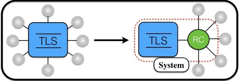
equa-TLS
RCSystem
[image:3.612.56.304.54.138.2]TLS
FIG. 1. Schematic of the reaction coordinate mapping, show-ing a two-level-system (TLS) coupled directly to an oscillator environment (left), which is mapped to a TLS coupled to the reaction coordinate (RC) plus a residual bath (right).
tions57–65, they may again be restricted; for example to
situations in which the high-frequency environmental re-sponse dominates59,66–68.
Recently, a master equation approach based on the reaction coordinate (RC) model (see Fig. 1) was intro-duced to describe the dynamical behaviour of a system coupled to an environment with strong low-frequency components, leading to long environmental correlation times18. Here, a collective coordinate of the bath 69–77
is incorporated into an enlarged effective system Hamil-tonian. This allows for the derivation of a second-order master equation for the dynamics of the reduced sys-tem and RC, accurately describing the syssys-tem dynamics even in the presence of strong system-environment corre-lations and extended environmental memory. Apart from its conceptual simplicity, the reaction coordinate master equation (RCME) is attractive due to the additional in-sight that it provides beyond the system, into both the environmental dynamics and the generation of system-environment correlations18.
In this work, we shall employ the RCME to inves-tigate EET in a molecular dimer system beyond weak system-environment coupling. We shall show that over the broad regimes considered, the RC model captures all important system-environment correlations for EET in the presence of both underdamped and overdamped environments, agreeing perfectly with numerically ex-act data generated using the HEOM44–47. Furthermore,
we demonstrate that the RC model significantly outper-forms the closely related Zusman equations72,75,78, a set of drift-diffusion equations often used to describe tun-nelling processes in molecular systems, which we derive from the RCME in a semiclassical limit. We also exam-ine the role that a structured environment may play in the dimer energy transfer dynamics. This is achieved in a consistent and non-perturbative manner by incorporat-ing an underdamped mode into the system Hamiltonian using the RC formalism, while the broad background en-vironment is described using a second overdamped RC. We show that the presence of structure in the spectral density can enhance the EET rate in specific regimes, in particular when the characteristic frequency of the un-derdamped environment coincides with the excitonic res-onance of the molecular dimer. However, there are also
large regions of parameter space where no enhancement is to be expected.
The paper is organised as follows. In Section II we define the molecular dimer Hamiltonian and outline the RC mapping. In Section III we formulate the RCME, from which we also derive the well-established Zusman equations72,75,78. In Section IV we explore the dynamics
of the model for both overdamped and underdamped en-vironmental spectral densities using the RCME and Zus-man equations, which we benchmark against the HEOM technique. In Section V we extend our discussion to a structured environment, with a particular focus on the effect of environmental structure on the rate of energy transfer between the dimer sites. We summarise in Sec-tion VI and present further details of the Zusman equa-tions in the Appendix.
II. SYSTEM HAMILTONIAN AND THE REACTION COORDINATE MAPPING
We consider energy transport in a molecular dimer system, each site of which has an excited state |Xji
(j= 1,2) with an associated energyεj, and ground state |0ji. The two sites are coupled to each other via a
transi-tion dipole interactransi-tion, with strength ∆, and to separate harmonic environments, leading to a Hamiltonian of the form (where we set~= 1)
H=X
j
εj|XjihXj|+
∆
2 (|X102ih01X2|+|01X2ihX102|)
+X
j
|XjihXj| X
k fj,k
c†j,k+cj,k
+X
j,k
ωj,kc†j,kcj,k.
(1)
Here, c†j,k and cj,k are, respectively, the creation and
annihilation operators for the kth mode of the
envi-ronment at site j, and fj,k is the corresponding
cou-pling strength. To simplify the analysis, we assume that the couplings between each site and its environ-ment are identical, then rotate the coordinate system such that the two sites couple directly to a single bath within the single excitation subspace spanned by the ba-sis{|1i=|X102i,|2i=|01X2i}. Restricting ourselves to
the single exciton subspace allows us treat the dimer as an effective two level system (TLS), and we can then write the Hamiltonian in spin-boson form
HSB= ǫ
2σz+ ∆
2σx+σz
X
k fk
˜
c†k+ ˜ck
+X
k
νk˜c†k˜ck,
(2)
where ǫ = ǫ1 − ǫ2, ˜ck = 21(c1,k−c2,k), and fk = f1,k/
√
2. We have also introduced the Pauli operators,
σz = |1ih1| − |2ih2| and σx = |2ih1|+|1ih2|. We can
is a measure of coupling strength weighted by the envi-ronmental density of states.
Given that our Hamiltonian is now in spin-boson form, the derivation of the RCME proceeds as in Ref.18, which
we shall summarise here for completeness. To move beyond the weak-coupling limit appropriate to Born-Markov (e.g Redfield) master equations we apply a nor-mal mode transformation to Eq. (2), incorporating a col-lective environmental degree of freedom into a new effec-tive system Hamiltonian. Following the method outlined by Garg et al.71, we define a collective mode of the
envi-ronment, known as the RC, which couples directly to the TLS. The RC is in turn coupled to a residual harmonic environment, as can be seen schematically in Fig. 1. This leads to a Hamiltonian of the form
HRC=HS+HI+HB+HC, (3)
with
HS= ǫ
2σz+ ∆
2σx+λσz a
†+a
+ Ωa†a,
HI= a†+a
X
k gk
b†k+bk
,
HB=
X
k
ωkb†kbk,
HC= a†+a
2X
k g2
k ωk ,
where the collective coordinate is defined such that
λ aˆ†+ ˆa
=X
k fk
˜
c†k+ ˜ck
. (4)
In Eq. (3) we have added a term, HC, quadratic in the
position operator of the RC, which removes the renor-malisation of the mode potential due to friction75. We
have also defined new creation and annihilation opera-tors, ˆb†k and ˆbk, respectively, for the residual bath. This
couples directly to the RC and is characterised by a new spectral density,JRC(ω) =Pk|gk|2δ(ω−ωk).
To describe the action of the residual bath on the RC we need to relate this spectral density to the original spin-boson spectral densityJSB(ω). To do so, we replace
the TLS with a classical coordinateqsubject to a poten-tial V(q)71,74. By considering the Fourier transformed
equations of motion for the coordinate, both before and after the mapping, we gain expressions of the form18
˜
K(z)˜q(z) =−V˜′(q), (5)
where tildes refer to Fourier transforms and prime de-notes the derivative with respect toq. For example, af-ter the RC mapping, the Fourier space operator may be written as
˜
K(z) =−z2+2λ Ω
L(z)
Ω2+L(z), (6)
� ��� ��� ��� ��� ���
��� ��� ��� ��� ��� ���
ω(��-�)
���
(
ω
)
(�)
� ��� ��� ��� ��� ���
� � �� �� ��
ω(��-�)
���
(
ω
)
(�)
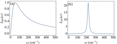
FIG. 2. Example spectral densities considered in this work: (a) Overdamped spectral density with ωc = 53 cm
−1 and
πα= 2 cm−1
; (b) Underdamped spectral density with πα= 2 cm−1, Γ = 20 cm−1, andω
0= 220 cm−1.
with L(z) = −z2 −4Ωz2R∞
0
JRC(ω)
ω(ω2−z2)dω. Finally, the
spin-boson spectral density may be related to JRC(ω)
using the Leggett prescription79:
JSB(ω) =
1
πǫlim→0+Im
˜
K(ω−iǫ). (7)
In the following we shall study two spectral densities rel-evant to EET systems, the underdamped (UD) and over-damped (OD) Brownian oscillator forms
JUD SB(ω) =
αUDΓω20ω
(ω2
0−ω2)2+ Γ2ω2
, (8)
and
JSBOD(ω) =αODωc ω ω2+ω2
c
. (9)
By choosing the RC spectral density to have the form
JRC(ω) =γωexp (−ω/Λ), and using Eq. (7) in the limit
that Λ→ ∞, we find the relation
JSB(ω) = 4γωΩ 2λ2
(Ω2−ω2)2+ (2πγΩω)2. (10)
Thus the mapping described above is exact for the under-damped spectral density when Ω =ω0,λ=
p
παUDω0/2,
andγ = Γ/2πω0. We can also recover the overdamped
spectral density by choosingγ such that ωc≪Ω, where
the RC coupling strength and frequency satisfy
ωc=
Ω
2πγ and αOD=
2λ2
[image:4.612.317.564.50.144.2]πΩ. (11)
Fig. 2 gives illustrative examples of the spectral densi-ties defined in Eqs. (8) and (9), demonstrating that in comparison to the broader overdamped limit, the under-damped case displays a sharp peak centred about the characteristic frequency ω0. A combination of the two
III. DYNAMICAL EVOLUTION IN THE RC MODEL
By mapping the spin-boson Hamiltonian of Eq. (2) to the RC form given in Eq. (3), we are now in a position to proceed with the dynamical description of our dimer system. We shall consider two related approaches. In the first we derive the full RCME (a quantum master equa-tion) for the reduced dynamics of both the dimer and the RC, while in the second we apply further approximations in order to derive a set of partial differential equations (PDEs), known as the Zusman equations.
A. Reaction coordinate master equation
We consider a second-order master equation for the re-duced state of the RC and TLS, ρ(t). This accounts for the TLS-RC coupling exactly, while treating interactions with the residual environment perturbatively to second order. This treatment will be valid when the coupling between the mapped system and the residual environ-ment is weak and/or when the environenviron-mental correlation time is short. From Eq. (3), moving into the interac-tion picture with respect toHS+HB, we may write the
Born-Markov master equation as56
∂ρI(t)
∂t =−i[HC(t), ρ(0)]
−
∞ Z
0
dτ trB[HI(t),[HI(t−τ), ρI(t)⊗ρB]],
(12)
where ρB = e−βHB/trB{e−βHB} is the reduced state of
the residual bath, which is assumed to remain in thermal equilibrium at temperature T = 1/β (forkB = 1). This
assumption is justified when the coupling between the residual bath and the composite system is small or the residual bath correlation time is very short. By follow-ing the derivation outlined in Ref.18, we may write the
Schr¨odinger picture master equation for the combined TLS and RC as
˙
ρ(t) =−i[HS, ρ(t)]
−γ
∞ Z
0 dτ
∞ Z
0
dω ωcosωτcothβω 2
h
ˆ
A,hAˆ(−τ), ρS(t)
ii
−γ
∞ Z
0 dτ
∞ Z
0
dωcosωτhA,ˆ nhAˆ(−τ), HS
i
, ρ(t)oi,
(13)
where we have defined ˆA= ˆa†+ ˆa.
The complexity of the system Hamiltonian makes gain-ing an analytic expression for the interaction picture operators difficult. However, by simply truncating the space of the collective coordinate up to n basis states,
i.e. limiting ourselves to n excitations in the RC, we can numerically diagonalise HS. This approach leads
to the set of basis states|ϕji which satisfy the relation HS|ϕji = ϕj|ϕji, allowing us to write the interaction
picture operators as
ˆ
A(t) =
2n X
j,k=1
Ajkeiωjkt|ϕjihϕk|, (14)
whereAjk=hϕj|ˆa†+ ˆa|ϕkiandωjk=ϕj−ϕk. We can
now evaluate the time and frequency integrals in Eq. (13) to give
∂ρ(t)
∂t =−i[HS, ρ(t)]− h
ˆ
A,[ ˆχ, ρ(t)]i+hA,ˆ nΞˆ, ρ(t)oi,
(15)
where we have defined the rate operators
ˆ Ξ = π
2
2n X
j,k=1
γωjkAjk|ϕjihϕk|, (16)
ˆ
χ= π 2
2n X
j,k=1
γωjkcoth βωjk
2 Ajk|ϕjihϕk|, (17)
and assumed the imaginary parts (i.e. Lamb shifts) to be negligible. Eq. (15) thus captures the interaction between the TLS and RC non-perturbatively, while the residual bath is treated in a purely Markovian fashion.
B. Zusman Equations
From the RCME given in Eq. (13), we can derive a set of drift-diffusion PDEs by way of further approxima-tions. Specifically, the interaction picture operators in Eq. (13) are expanded using the Caldeira-Leggett ap-proach56,71,72,80, in which the system evolution is
as-sumed to be much slower than that of the environment, giving
ˆ
A(t) =e−iHStAeˆ iHSt
≈Aˆ+ithHS,Aˆ
i
. (18)
By inserting this approximate form into Eq. (13) we can evaluate the frequency and time integrals. We then move to a phase-space representation for the master equation by way of the Wigner transformation, leading to a gen-eralised Fokker-Plank equation in Klein-Kramers form81
∂Wˆ
∂t +HWˆ+(iZ −Ω 2x)∂Wˆ
∂p +p ∂Wˆ
∂x
=πγΩ∂
∂t pWˆ +
1
β ∂Wˆ
∂p !
where ˆW = P
ijWij(x, p, t)|iihj|, with i, j = 1,2. The
Wigner function is defined as
Wij(x, p, t) =
1 2π
∞ Z
−∞
dx′e−ipx′
i, x+x
′
2
ρ
x−x
′
2, j
,
(20)
where x and p are the phase-space coordinates of the RC. For brevity, we have defined the superoperators in
Eq. (19) as
HWˆ =ih(ǫ+√2Ωλx)σz+ ∆σx,Wˆ i
, (21)
Z∂∂pWˆ = i
√
2Ωλ
2
( σz,
∂Wˆ ∂p
)
. (22)
In its current form Eq. (19) remains challenging to solve. We may simplify it, however, by eliminating the momentum coordinate in the differential equation. We do this by assuming that the RC momentum remains in thermal equilibrium at all times, which is valid in the high friction limit. This enables us to expand the Wigner function in terms of Hermite polynomials, resulting in a hierarchy of equations (a detailed account of this deriva-tion can be found in the Appendix). By taking terms that are first order in the inverse friction (η−1, where η =πγΩ), we acquire a set of drift-diffusion equations, commonly referred to as the Zusman equations:
∂µ11(t, x)
∂t =
1 2πγΩ
∂ ∂x
1 β
∂µ11(t, x)
∂x + (Ω
2x+√2Ωλ)µ 11(t, x)
+i∆(µ12(t, x)−µ21(t, x)), (23)
∂µ22(t, x)
∂t =
1 2πγΩ
∂ ∂x
1 β
∂µ22(t, x)
∂x + (Ω
2x+√2Ωλ)µ 22(t, x)
−i∆(µ12(t, x)−µ21(t, x)), (24)
∂µ12(t, x)
∂t =
1 2πγΩ
∂ ∂x
1 β
∂µ12(t, x)
∂x + Ω
2xµ 12(t, x)
+ 2i(ǫ 2 +
√
2Ωλx)µ12(t, x) +i
∆
2(µ11(t, x)−µ22(t, x)), (25)
∂µ21(t, x)
∂t =
1 2πγΩ
∂ ∂x
1 β
∂µ21(t, x)
∂x + Ω
2xµ 21(t, x)
+ 2i(ǫ 2 +
√
2Ωλx)µ21(t, x)−i
∆
2(µ11(t, x)−µ22(t, x)), (26)
where µij(t, x) describes the time evolution of both the
TLS and the RC with respect to the phase-space variable
x. We can then extract the time evolution of the TLS population [ρ11(t)] and coherence [ρ12(t)] using
ρ11(t) =
∞ Z
−∞
µ11(t, x)dx and ρ12(t) =
∞ Z
−∞
µ12(t, x)dx.
The Zusman equations describe a mode in the high fric-tion limit and are based on approximafric-tions that amount to a semiclassical treatment of the RC, in which quantum correlations between the RC and dimer are neglected. One may extend their validity by considering higher order terms. However, the equations quickly become unwieldy and computationally impractical in the low friction limit. Thus, we shall restrict ourselves to the first-order equa-tions here.
IV. SYSTEM DYNAMICS
To explore the system dynamics using the RCME [Eq. (15)], we assume that the dimer and RC are
ini-tially uncorrelated at time t = 0, with the RC in a thermal state and an excitation localised at dimer site 1 (unless otherwise stated). That is,ρ(0) =Z−1|1ih1| ⊗
exp −βΩa†a
, where Z = tr
exp −βΩa†a . For the
Zusman equations, this gives the boundary condition
µ11(0, x) = 2
v u u ttanh
βΩ
2
π e
−Ω tanh(β2Ω)x 2
, (27)
while µ22(0, x) = µ21(0, x) = µ12(0, x) = 0. We
shall compare the dynamical behaviour predicted by the RCME and Zusman equations, solved numerically82,83,
● ●● ●● ●● ● ● ●● ● ● ●● ● ● ●● ● ● ●● ● ● ●● O O O O O O O O O O O O O O O O O O O O O O O O O O O ��� ��� ��� ��� ��� ��� ��� ��� ��� ��� ��� ��� ����� �(��) ρ�� ( � )
(�)πα��=� ��-�
● ● ● ● ● ● ● ● ● ● O O O O O O O O O O O ��� ��� ��� ��� ��� ��� ��� ��� ��� ��� ��� ��� ��� ����� �(��) ρ�� ( � )
(�)πα��=��� ��-�
● ● ● ● ● O O O O O O � ��� ��� ��� ��� ��� ���� ���� ���� ����
�������� ���������πα��(��-�) ρ�� ( ∞ ) (�)�=��� � ● ● ● ● ● O O O O O ����� ����� ����� ����� ����� ����� � � � �
������� ������������β(��-�)
ρ�� ( ∞ )/ ρ�� ( ∞ )
(�)πα��=��� ��-�
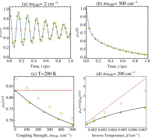
FIG. 3. (a,b) Comparison of the dimer site population dynam-icsρ11(t) calculated from the RCME (solid curves), Zusman
equations (open-points) and the HEOM (solid-points) for the coupling strengths indicated andT = 300 K. (c) Steady-state population in the dimer eigenstate basis (upper eigenstate, ρee(t)) as a function of system-environment coupling strength for all three theories and the canonical equilibrium state (dot-dashed). (d) Variation of the dimer eigenstate population ra-tio against inverse temperature for all three theories. The other parameters are ∆ = 200 cm−1, ǫ = 100 cm−1, and
ωc= 53.08 cm −1
A. Overdamped spectral density
In Fig. 3 (a) and (b) we compare the short time pop-ulation dynamics of site 1 as predicted by the RCME (solid curves), Zusman equations (open points) and the HEOM (solid points). We consider an overdamped envi-ronment and take parameters representative of a subset of the Fenna-Matthews-Olson complex84. We find
excel-lent agreement between the RCME, Zusman equations, and the HEOM at both weak and strong coupling to the environment in this regime, capturing the transition from coherent to incoherent energy transfer57. It is evident
that by including the RC into the system Hamiltonian, we are able to faithfully represent all relevant system-environment correlations in the dimer evolution. More-over, for this overdamped spectral density, the residual environmental influence is sufficiently strong to suppress significant oscillations in the RC degrees of freedom. We are therefore in the high friction limit, and the Zusman equations are expected to provide a good description of the system dynamics on transient timescales.
1. Non-canonical equilibrium states and the dynamical generation of correlations
Nevertheless, the semiclassical approximations inher-ent within the Zusman treatminher-ent still manifest them-selves on longer timescales, as demonstrated in Fig. 3 (c) and (d). Here, we see that they cannot correctly capture the equilibration behaviour of the system in the long-time limit. For example, at a temperature ofT = 200 K, the Zusman equations clearly do not lead to the correct steady-state population in the excitonic basis (i.e. the eigenbasis of ǫ
2σz + ∆
2σx), even for very weak
system-environment coupling strengths. Interestingly, with in-creasing coupling strength (or dein-creasing temperature), the steady-states derived from both the RCME and the HEOM deviate noticeably from the canonical thermal state; that is, the state
ρSth= e−β(ǫ
2σz+∆2σx)
ZC
, (28)
where ZC = trS
n e−β(ǫ
2σz+ ∆ 2σx)
o
. As shown in Ref.18,
this is a consequence of significant and long lasting cor-relations accumulated between the system and environ-ment at both weak and strong coupling, with the re-sult that the canonical thermal state no longer describes the true equilibrium state of the system. Though such steady-state correlations are correctly captured through the RCME, they are not in the Zusman equations. Hence, we find that it is necessary to retain a full quantum treat-ment of the dimer-RC interaction within the RCME to accurately describe our system over all timescales. In fact, the steady-state of the RCME may be compactly expressed instead as a canonical thermal state with re-spect to the full RC Hamiltonian
ρ(t→ ∞) = e
−β(ǫ
2σz+∆2σx+λσz(a†+a)+Ωa†a) ZN C
, (29)
where ZN C = tr n
e−β(ǫ
2σz+∆2σx+λσz(a†+a)+Ωa†a)o. On
tracing over the RC or TLS, this represents a non-canonical dimer equilibrium state or a non-thermal envi-ronmental state, respectively. The former may be bench-marked against the HEOM, and proves to accurately cap-ture deviations in the steady-state of the dimer due to system-environment correlations18. Of course, the
influ-ence of correlations is also dependent on the temperature of the bosonic environment. Fig. 3 (d) demonstrates that at very large temperatures the steady-states obtained from the RCME, the HEOM, and the Zusman equations begin to agree, converging towards the canonical ther-mal state. Here we enter a regime in which the quantum correlations shared between the system and environment are suppressed, such that the semiclassical approxima-tion is adequate to describe the dimer behaviour even at relatively strong system-environment coupling.
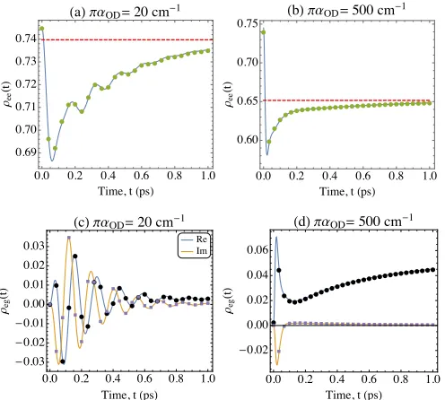
[image:7.612.57.299.51.275.2]●
● ●
● ● ●●●
● ● ●● ● ● ●● ● ● ●
● ● ● ●● ● ●
��� ��� ��� ��� ��� ��� ����
���� ���� ���� ���� ����
����� �(��) ρ��
(
�
)
(�)πα��=�� ��-�
●
● ●●●
●●●●●●●●●●●●●●●●●●●●●●●●●●
��� ��� ��� ��� ��� ���
���� ���� ���� ����
����� �(��)
ρ��
(�
)
(�)πα��=��� ��-�
● ●
● ●
●
● ●
● ●
●●
● ●
●● ● ●●●●●●●●●●
■
■ ■
■
■
■ ■ ■
■■ ■
■ ■■
■
■ ■ ■ ■ ■ ■ ■ ■ ■ ■ ■ �� ��
��� ��� ��� ��� ��� ��� -����
-���� -���� ���� ���� ���� ����
����� �(��)
ρ��
(
�
)
(�)πα��=�� ��-�
● ●
●
●●●●●●●●
●●●●●●●●●
●●●●●●●●●●●
■
■
■■■■■■■■■■■■■■■■■■■■■■■■■■■■■
��� ��� ��� ��� ��� ���
-����
���� ���� ���� ����
����� �(��) ρ��
(
�
)
[image:8.612.325.554.48.343.2](�)πα��=��� ��-�
FIG. 4. Top: Excitonic upper eigenstate population dynam-ics, ρee(t), for a system initiated in its canonical thermal state given in Eq. (28). The solid curve is calculated with the RCME and the points are obtained from the HEOM. The dashed lines represent the non-canonical system steady-state given by tracing over the RC in Eq. (29). Bottom: The corresponding real and imaginary parts of the coher-ence in the dimer excitonic eigenbasis calculated using the RCME (solid) and the HEOM (points). The other parame-ters areωc= 53.08 cm
−1, ∆ = 200 cm−1,ǫ= 100 cm−1, and
T = 300 K.
For example, consider a system that is initially in (quasi) equilibrium with its surrounding environment, before be-ing perturbed by an external field. Na¨ıvely, one might assume that the initial state of the system in this situa-tion should be the canonical thermal state with respect to the internal system Hamiltonian. Our previous argu-ments, however, demonstrate that this assumption may be misleading in the context of our molecular dimer sys-tem, as shown explicitly in Fig. 4. Here, we consider the dynamical evolution of the dimer in its excitonic eigenba-sis, when the system is initiated in the canonical thermal state given by Eq. (28). We see that the subsequent dynamics can display coherent oscillations in the dimer eigenbasis and even the generation of excitonic coher-ences, before relaxation to an equilibrium state that dif-fers from the initial thermal state. Note that this is true even when the equilibrium state is close to the canonical state, as in the left panels of the figure.
Behaviour of this kind is markedly different to that expected from less sophisticated master equation tech-niques in which the system-environment coupling is treated perturbatively. Often, such approaches lead to a complete absence of dynamical evolution in the dimer eigenbasis for a system initialised in a canonical thermal state, since Eq. (28) is the expected equilibrium steady-state when the environmental influence is a weak
pertur-●
●
● ●
●
● ●
●● ●
●
● ●● ● ●● ● ● ● ● ● ● ● ● ● ● ● ● ●
��� ��� ��� ��� ��� ���
��� ��� ��� ��� ��� ��� ���
�����(��) ρ��
(
�
)
��� ��� ��� ��� ��� ��� ���
��� ��� ��� ���
�(��)
ρ��
(
�
)
●
●
● ●
●●●●
● ●
●
● ●
● ●
● ● ●●●● ● ● ● ● ● ● ● ● ●
��� ��� ��� ��� ��� ���
��� ��� ��� ���
�����(��)
ρ��
(
�
)
��� ��� ��� ��� ��� ��� ���
��� ��� ��� ���
�(��) ρ��
(
�
)
FIG. 5. Dimer site population dynamics for an underdamped spectral density with (top)ω0= 40 cm−1,παUD= 20 cm−1,
and (bottom) ω0 = 220 cm−1, παUD = 10 cm−1. In
the main plots we compare the RCME (solid curves) and HEOM (points), while results from the Zusman equations are shown in the insets. Dashed lines denote the non-canonical steady-state values (reached on a very slow timescale for the top plot). The other parameters are ∆ = 200 cm−1,
ǫ= 100 cm−1, Γ = 10 cm−1, andT = 300 K.
bation.
B. Underdamped spectral density
We shall now move on to discuss the impact of an underdamped spectral density on the EET dynamics of our dimer. The resultant complex system dynamics have particular relevance to EET in the presence of structured environments, where the system may be strongly cou-pled to specific lossy modes that dominate regions of the pigment-protein vibrational spectrum.
[image:8.612.49.297.51.274.2]Con-� � � � � � � �
-���
-���
-���
��� ��� ��� ���
����� �(��)
〈
�
〉 -����� � � � � � � �
� ����
〈
�
〉
� � � � � �
-���
-���
��� ��� ��� ��� ���
����� �(��)
〈
�
〉
� � � � � �
-����
� ����
〈
�
[image:9.612.61.293.50.350.2]〉
FIG. 6. The RC position (main) and momentum (inset). Top: ω0= 40 cm−1andπαUD= 20 cm−1. Bottom: ω0= 220 cm−1
andπαUD= 10 cm−1. Other parameters are the same as in
Fig. 5.
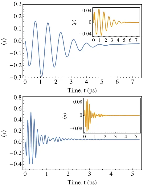
sidering, for example, the low frequency spectral density, when one compares the RC frequency (Ω = 40 cm−1)
to the friction acting on the mode (η ≈ 5 cm−1,
ob-tained from the mapping) we find that the RC is weakly damped. Hence, the limits taken to derive the Zusman equations are invalid, i.e. the momentum of the RC does not remain in thermal equilibrium in this regime. This is shown explicitly in Fig. 6, where we plot the dynami-cal evolution of the RC positionhxˆ(t)i= tr{xρˆ (t)}, and momentumhpˆ(t)i= tr{pρˆ (t)}, defined as
ˆ
x=
r
1 2Ω(a
†+a) and pˆ=i r
Ω 2(a
†−a). (30)
We see pronounced oscillations at several frequencies in both the RC position and momentum, which are grad-ually damped at long times, equilibrating to non-zero values consistent with the state given in Eq. (29).
The disagreement between the Zusman equations and the RC model is further exacerbated when the under-damped spectrum is tuned close to the dimer resonance,
ζ=√ǫ2+ ∆2≈223 cm−1. As can be seen in Fig. 6 (b),
the RC now undergoes even larger amplitude oscillations. In this case the Zusman equations are completely unable to capture the dynamical behaviour of the system, pre-dicting only rapid oscillations in the dimer population.
� ��� ��� ��� ���
���� ���� ���� ���� ���� ����
ω(��-�)
�
(ω
)
� ��� ��� ��� ���
����� ����� ����� ����� ����� �����
ω(��-�)
�
(ω
)
FIG. 7. Fourier transform of the RCME population dynamics in Fig. 5, demonstrating the presence of multiple oscillation frequencies. Left: ω0= 40 cm−1. Right: ω0= 220 cm−1.
The RCME, on the other hand, shows excellent agree-ment with the HEOM for both short and long times, cap-turing perfectly the population dynamics of the dimer. In both the low and high frequency cases, the dimer dy-namics displays complex beating behaviour, with multi-ple oscillation frequencies. From the RC formalism we have a clear interpretation for this behaviour in terms of the strong oscillations experienced by the collective coordinate of the environment, which in turn leads to modulations of the TLS dynamics.
This is shown explicitly in Fig 7, where we have taken the Fourier transform of the population dynamics given in Fig. 5, that is
S(ω) = Re
∞ Z
0
dteiωt(ρ11(t)−ρ11(t→ ∞))
. (31)
Here, we have subtracted the steady-state population,
ρ11(t→ ∞), to remove aδ-function contribution. For the
lower frequency underdamped environment (left plot) we see the presence of two specific frequencies in the spec-trum, one at the RC mode frequency (ω0 = 40 cm−1),
and the other at the dimer splitting (ζ ≈ 223 cm−1).
When the characteristic frequency of the spectral den-sity approaches the dimer splitting (right plot) we see further structure in the oscillation spectrum, with the emergence of additional peaks. Again, we may explain this by appealing to the physical intuition gained from the RC model. In this case, the environmental response, and thus RC splitting, lies close to the resonant frequency of the dimer, leading to an effective enhancement of the interaction between the dimer and RC. As a result of the enhanced coupling, the spectrum of the system can-not be associated to the bare frequencies of the dimer and RC, but rather to the eigenstates of the composite system. Hence, we see a double peak structure about
ω∼220 cm−1, split by the RC-dimer coupling strength
2λ= 66 cm−1. This is reminiscent of the vacuum Rabi
splitting observed in cavity QED systems, in which the eigenstates of the system are the light-matter entangled dressed states85.
[image:9.612.312.560.51.146.2]◆
◆◆ ◆ ◆ ◆ ◆ ◆ ◆ ◆ ◆ ◆ ◆ ◆ ◆ ◆◆ ◆ ◆ ◆ ◆ ω�=����-�
ω�=����-�
ω�=�����-�
� �� ��� ��� ��� ��� ���
� �� �� �� ��
ω(��-�)
�
(
ω
)
◆
◆
◆◆◆ ◆◆◆
◆◆◆◆◆◆◆◆◆◆◆◆◆◆◆◆◆◆◆◆◆◆◆
� ��� ��� ��� ��� ����
��� ��� ��� ��� ��� ��� ���
����� �(��) ρ��
(
�
[image:10.612.55.303.51.146.2])
FIG. 8. Left: Underdamped (curves) and overdamped (points) spectral densities for several environmental frequen-cies. Right: The population dynamics associated to these spectral densities. Here, we see a smooth transition from the underdamped (curves) to overdamped (points) regime for in-creasing ω0. The parameters are the same as Fig. 5, with
Γ =ω20ω
−1
c , andπα= 100 cm −1
.
particular, the discussion above demonstrates that it is not straightforward to assign electronic and vibrational frequencies in situations where underdamped modes are present, as one must also account for the coupling be-tween the molecular dimer and any such modes, which leads to the formation of vibronic states.
As a final remark, we can show that the RC model for an underdamped spectrum convergences to the over-damped case in regimes where Γ, ω0≫1. We do this by
defining a cut-off frequency in the underdamped spec-trum as ωc =ω20/Γ, which sets the energy scale of the
overdamped spectrum in the appropriate limit. Using this definition we fix Γ =ω2
0/ωc and consider the
under-damped spectrum for increasing ω0 as demonstrated in
Fig. 8. Here we see a smooth transition between the un-derdamped and overdamped regimes, with the two agree-ing well at largeω0.
V. STRUCTURED ENVIRONMENTS
Having established the validity and potential for physi-cal insight of the RCME when applied to overdamped and underdamped environments separately, in this section we explore how a structured environment impacts upon the energy transfer rate in a molecular system. To do this in a consistent manner, we shall consider the dynam-ics of a dimer coupled to a broad background environ-ment described by an overdamped spectral density, with structure incorporated via a second underdamped envi-ronment with peak centred around ω0. We shall model
both environments using the RC mapping outlined previ-ously, extracting an independent RC for each, allowing us to rigorously account for dissipation on the underdamped mode. Furthermore, our enlarged system (see left plot of Fig. 9) naturally captures the vibronic nature imparted on the dimer byboththe underdamped and overdamped
components of the environmental spectrum.
The Hamiltonian describing the system and
environ-ments may be written as
HST=HD+σz 2
X
i=1
X
k
fk(i)(ci,k+c†i,k) +HB, (32)
withHB=P k
ω(ki)c†i,kci,kandHD= ǫ2σz+∆2σx. The two
environments are characterised by the spectral densities
Ji(ω) = X
k
|fk(i)|2δ(ω−ω(ki)), (33)
withJ1(ω) =JOD(ω) and J2(ω) =JUD(ω). The
combi-nation of these terms leads to an effective spectral density with a broad background, given by the overdamped com-ponent, and a sharp peak associated to the underdamped contribution. Illustrative examples are given in the right hand plot of Fig. 9.
We shall assume that the two environments are initially uncorrelated with one another (e.g. in a thermal state), but are able to generate correlations through interactions mediated by the dimer. This allows each environment to be mapped to the RC model independently. Applying the mapping we obtain the system Hamiltonian
HS= ǫ
2σz+ ∆
2σx+σz
X
i λi
a†i +ai
+X
i
Ωia†iai, (34)
witha1 (a2) the annihilation operator of the RC
associ-ated with the underdamped (overdamped) environment. Each RC then couples to an independent residual envi-ronment, giving the interaction Hamiltonian
HI=
X
i
a†i+ai X
k
g(ki)b†i,k+bi,k
. (35)
Here, bi,k (b†i,k) is the annihilation (creation) operator
for thekthmode of each residual environment (i= 1,2),
which are characterised by the spectral densities ˜Ji(ω) = P
k|g (i)
k |2δ(ω−ω (i)
k ) =γiω. The parameters describing
the RCs can then be found in terms of the original spec-tral densities using the relations given in Section II.
By following the RCME derivation for each indepen-dent environment we obtain an equation of motion de-scribing the dynamics of the dimer TLS andbothRCs
∂ρ(t)
∂t =−i[HS, ρ(t)]− X
i h
ˆ
Ai,[ ˆχi, ρ(t)] i
+hAˆi, n
ˆ Ξi, ρ(t)
oi , (36)
with ˆAi = (a†i +ai), and the rate operators ˆχi and ˆΞi
defined in analogy to the single RC case in Eqs. (16) and (17).
TLS
OD UD
System
πα��
� � �� �� ��
� ��� ��� ��� ���
� � � � � ��
ω(��-�)
���
(ω
[image:11.612.337.540.48.312.2])
FIG. 9. Left: Schematic of the RC model for a structured environment with underdamped (UD) and overdamped (OD) components, each coupled to their own residual environment. Right: The structured spectral density at various reorgani-sation energies of the overdamped contribution. The under-damped RC has frequencyω0= 100 cm−1, with Γ = 20 cm−1
andπαUD= 2 cm−1.
caseǫ= 100 cm−1 and ∆ = 40 cm−1), we can do so by
defining a rate using the the classical equations84
dP1(t)
dt =−k1→2P1+k2→1P2, dP2(t)
dt =k1→2P1−k2→1P2.
(37)
Here, P1 (P2) is the population at dimer site 1 (2) and k1→2 (k2→1) is the transfer rate between sites 1 and
2 (2 and 1). These equations lead to purely exponen-tial decays of the dimer populations, thus neglecting all coherent contributions in the energy transfer dynamics. Though a coarse approximation, this procedure gives in-sight into the overall transfer rate, and is accurate in regimes where the tunnelling between sites is weak and coherent dynamics is consequently suppressed.
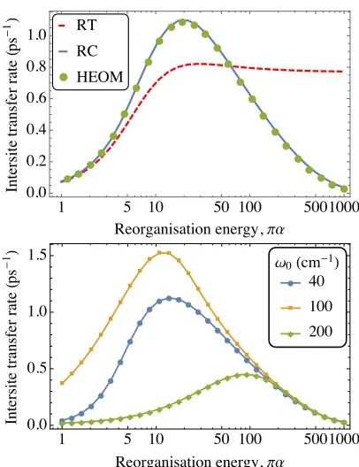
We first consider the case of a single overdamped envi-ronment84. In Fig. 10 (top) we plot the inter-site transfer
rate as a function of the reorganisation energy calculated from the RCME (solid curve), the HEOM (points), and a Redfield master equation (dashed curve) in which the system-environment coupling is treated perturbatively56.
We see that the RCME perfectly captures the smooth peak in the rate predicted by the HEOM as the reor-ganisation energy is increased. As has previously been shown59,84, Redfield theory fails even to qualitatively
capture this behaviour, plateauing at large reorganisa-tion energies. We may also explore the transfer rate in the presence of a single underdamped environment us-ing the RCME. As shown in Fig. 10 (bottom), much like the overdamped example, the EET rate in the under-damped case shows a peak at some intermediate cou-pling strength, the position and height of which is highly dependent on the characteristic frequency of the environ-ment. Specifically, the transfer rate reaches its maximum when the peak of the underdamped spectrum approaches the resonance of the dimer (ζ≈108 cm−1here). As was
discussed in Sec. IV B, when the dimer and the RC are close to resonant, the vibronic states of the composite system play a significant role in the system dynamics. In this case they act to increase the number of pathways
�� �� ����
� � �� �� ��� �������
��� ��� ��� ��� ��� ���
�������������� �������πα
���
���
���
���
��
��
���
��
(
��
-� )
● ●●
●●
● ●
●
●●
● ● ● ●●
● ●
● ●
● ●
● ●
● ● ●
● ● ● ●
■■ ■■
■ ■
■ ■
■■ ■ ■ ■■ ■
■ ■
■ ■
■ ■
■ ■
■ ■
■ ■■ ■ ■ ◆ ◆ ◆ ◆ ◆ ◆ ◆ ◆◆ ◆ ◆
◆ ◆◆ ◆
◆ ◆◆ ◆ ◆ ◆ ◆◆ ◆ ◆
◆ ◆◆◆ ◆ ω�(��-�)
● ��
■ ���
◆ ���
� � �� �� ��� ������� ���
��� ��� ���
�������������� �������πα
���
���
���
���
��
��
���
��
(
��
-�)
FIG. 10. Variation in dimer inter-site energy transfer rate k1→2 for increasing reorganisation energy. Top: Predictions
from the RCME (solid curve), the HEOM (points) and weak-coupling Redfield theory (RT, dashed curve) for a single over-damped environment. Both the RCME and HEOM pre-dict a smooth peak in the rate at intermediate reorganisa-tion energy, whereas the Redfield master equareorganisa-tion fails to capture the correct behaviour for all but the weakest cou-pling strengths. Bottom: RCME predictions for a single underdamped environment for several characteristic frequen-ciesω0, with Γ = 20 cm−1. Notice that the largest transfer
rates occur forω0 = 100 cm−1, which is close to the
reso-nance of the dimer TLS. Other parameters areǫ= 100 cm−1,
∆ = 40 cm−1,ω
c= 53 cm
−1, andT = 300 K.
available for energy to be transferred between the two sites of the dimer86, thus enhancing the EET rate.
[image:11.612.57.298.52.145.2]● ● ●
● ●
● ●
●
●
●
●
● ●
■ ■ ■ ■
■ ■ ■
■
■
■
■
■ ■ ◆ ◆
◆ ◆
◆
◆ ◆ ◆ ◆
◆
◆ ◆
◆ ▲ ▲
▲ ▲
▲
▲ ▲ ▲
▲
▲
▲ ▲
▲
▼ ▼▼
▼▼
▼ ▼
▼ ▼
▼
▼▼ ▼ ▼ ▼▼
▼ ▼
▼ ▼
▼ ▼
▼ ▼
▼
▼▼
� � �� �� ��� ���
��� ��� ��� ��� ��� ���
�������������� �������πα��
���
���
���
���
��
��
���
��
(
��
-�)
ω�(��-�)
● ��
■ ���
◆ ��� ▲ ���
▼ ��
●
●
● ●
● ● ● ● ● ● ● ● ●
■
■
■ ■
■ ■ ■ ■ ■ ■ ■ ■ ■
◆ ◆
◆ ◆
◆ ◆ ◆ ◆ ◆ ◆ ◆ ◆ ◆
▲ ▲
▲ ▲ ▲ ▲ ▲ ▲ ▲ ▲ ▲ ▲ ▲
� � �� �� ��� ���
� � � � �
�������������� �������πα��
���
��
��
��
���
��
��
���
ω�(��-�)
● ��
■ ���
[image:12.612.56.300.49.313.2]◆ ��� ▲ ���
FIG. 11. Enhancement of the dimer transfer rate due to envi-ronmental structure. The reorganisation energy of the under-damped component is kept constant atπαUD= 2 cm
−1 and
several frequencies ω0 are considered, while the
reorganisa-tion energy of the overdamped component is increased. Top: Intersite transfer rate as a function of overdamped reorgan-isation energy. For comparison, we have also included the transfer rate for a single overdamped environment. Bottom: Corresponding transfer enhancement, defined as the ratio of the rate with environmental structure to that of the single overdamped environment. For both plots the dimer and over-damped parameters are the same as Fig. 10. The under-damped environments have Γ = 20 cm−1 andT = 300 K.
the manifold of vibronic states. When it is tuned away from resonance, the effective coupling between the dimer and the underdamped RC is reduced, thus decreasing the amount of vibronic states that can be explored by the composite system, and consequently reducing the rate of EET. Note, however, that at large overdamped reorgani-sation energies the enhancement is suppressed regardless of the underdamped frequency, and the transfer rate fol-lows that of a single overdamped environment. This is true even when the underdamped component can still be clearly discerned within the spectral density (see Fig. 9), and is simply a consequence of the overdamped environ-ment becoming the dominant influence, such that the underdamped vibronic states have little effect even for a resonant mode. Thus, the presence of one or more well-resolved modes within the spectral density is not in itself sufficient to imply a vibronic enhancement of the dimer EET rate.
VI. SUMMARY
In summary, we have shown that the RCME provides a powerful, informative and intuitive method for describ-ing EET in molecular dimers – and more generally open quantum systems – for regimes in which the environmen-tal correlation time is long. It allows access to informa-tion on the system, its environment, and their correla-tions. Moreover, it greatly outperforms the closely re-lated semiclassical Zusman equations. This demonstrates that not only is the RC mapping important to capture the correct system behaviour, but also that one must prop-erly account for the correlations dynamically generated between the dimer and its environment through the RC. These correlations lead to complex system population dynamics comprising of multiple oscillation frequencies, which we interpret as feedback from the environmental collective mode. They also persist into the steady-state, pushing both the system and its environment away from their respective canonical equilibrium states in the long time limit.
We have applied the RC model to describe the be-haviour for overdamped, underdamped, and structured vibrational environments. In particular, we find that the presence of structure within the environment is capable of increasing the rate of EET between the dimer sites. This enhancement is dependent upon the energy scale of the underdamped vibrations within the environment, reaching its peak when they lie close to the dimer ex-citonic resonance as should be expected. Nevertheless, even for such resonance conditions, there are also regions of parameter space in which the structured environment offers no advantage in terms of an increased transfer rate, and the dynamics follows that determined by the broad overdamped background. It would thus be extremely in-teresting to apply the RCME to analyse such subtleties in larger molecular systems, with the aid of a suitable truncation scheme to limit the required number of basis states.
VII. ACKNOWLEDGEMENTS
Appendix A: The Zusman equations
In this Appendix we shall give further details on the derivation of the Zusman equations. Starting from the Caldeira-Leggett master equation in Wigner space we have87
Ωπγ ∂
∂p pWˆ +
1
β ∂Wˆ
∂p !
=∂Wˆ
∂t +HWˆ +iZ ∂Wˆ
∂p
+p∂Wˆ ∂x −Ω
2x∂Wˆ
∂p , (A1)
where we have defined the superoperators
HWˆ =i ǫ
2+κx
σz+
∆ 2σx,Wˆ
,
Z∂∂pWˆ =iκ 2
( σz,
∂Wˆ ∂p
)
. (A2)
We aim to simplify this equation of motion by remov-ing the momentum coordinate, in particular by assum-ing that the momentum of the RC remains in thermal equilibrium throughout the evolution of the system.
To eliminate the momentum coordinate from Eq. (A1) we shall use the procedure outlined by Coffey87, and
orig-inally formulated by Brinkman for the case of a Brownian oscillator88. We expand the Wigner function in terms of
Hermite polynomials
ˆ
W =e−µ2/4
∞ X
n=0
Dn(µ) ˆφn(x, t), (A3)
where we have rescaled the momentum coordinate such thatµ=√βp. The function ˆφ(x, t) is a two-by-two ma-trix describing the electronic dependence of the Wigner function andDn(µ) is the set of orthogonal Weber
func-tions, which are given by
Dn(y) = 2−n/2e−y 2
/4H n
y
√
2
,
where Hn(z) are the Hermite polynomials. The Weber
functions satisfy the following relations
Dn+1(y)−yDn(y) +nDn−1(y) = 0, (A4)
∂yDn(y) +y
2Dn(y)−nDn−1(y) = 0, (A5)
∂yDn(y)− y
2Dn(y) +Dn+1(y) = 0, (A6)
∂2yDn(y) +
n+1 2 −
y2
4
Dn(y) = 0, (A7)
∞ Z
−∞
Dn(y)Dm(y)dy=n! √
2πδm,n. (A8)
Substituting these expressions into the phase-space master equation given in Eq. (A1), and integrating
over our scaled momentum coordinate µ, we obtain the Brinkman hierarchy
∂φˆm
∂t +Hφˆm+
1
√
β
∂φˆm−1
∂x + (m+ 1) ∂φˆm+1
∂x !
+pβΩ2xφˆm−1+πγΩmφˆm− p
βZφˆm−1= 0.
(A9)
We also define the differential operators
J =− √
β η
1
β ∂ ∂x + Ω
2x −iZ
,
JD=−
1
η√β ∂ ∂x,
(A10)
which allows us to write
1
η ˙ˆ
φm+Hφˆm
+mφˆm=Jφˆm−1+ (m+ 1)JDφˆm+1,
whereη=πγΩ quantifies the friction acting on the mode. We now move to Laplace space with respect to the time coordinate, using the transformation
˜
ϕn = ˜ϕn(x, s) =
∞ Z
−∞
ˆ
φn(x, t)e−stdt, (A11)
which leads to the relation
∂φˆn ∂t
LT
=⇒sϕ˜n−φˆn(x,0). (A12)
For a mode initially in a thermal state, the initial condi-tions of the system are entirely determined by ˆφ0(x,0),
such that ˆφn(x,0) = 0 forn >0, leading to the following
hierarchy of equations in Laplace space:
1
η
sϕ˜0+ ˆφ0(x,0) +Hϕ˜0
=JDϕ˜1,
1
η (sϕ˜1+Hϕ˜1) + ˜ϕ1=Jϕ˜0+ 2JDϕ˜2,
1
η (sϕ˜2+Hϕ˜2) + 2 ˜ϕ2=Jϕ˜1+ 4JDϕ˜3,
.. .
We can close these equations by assuming ˜ϕ3= 0 (which
is consistent with keeping terms to leading order inη−2)
and hence solve for ˜ϕ0. Inverting the equation for ˜ϕ2,
˜
ϕ2= J
˜
ϕ1 1
η(s+H) + 2
, (A13)
and substituting this into the equation for ˜ϕ1gives
˜
ϕ1= J
˜
ϕ0 1
η(s+H) + 1 + 2JDJ
1
η(s+H)+2
which leads to the equation
1
η
sϕ˜0+ ˆφ0(x,0) +Hϕ˜0
= JDJϕ˜0 1 + 1η(s+H) + 2JDJ
1
η(s+H)+2
.
In the very large damping limit, the friction coefficientη
is much larger than any other scale. Hence, we can keep terms only to leading order in the inverse friction η−1,
giving
sϕ˜0+ ˆφ0(x,0) +Hϕ˜0=ηJDJϕ˜0. (A15)
Inverting the Laplace transform we therefore have
∂φˆ0 ∂t =−i
ǫ
2 +κx
σz+
∆ 2σx,φˆ0
+ηJDJφˆ0. (A16)
Finally, we can decompose φ0 in terms of the dimer
states, such that ˆφ0=P2i,jµij(x, t)|iihj|, whereµij(x, t)
describes an element of the dimer density matrix and is dependent on the RC position. Substituting into Eq. (A16) we obtain the Zusman equations
∂µ11(t, x)
∂t =
1 2πγΩ
∂ ∂x
(Ω2x+κ)µ11(t, x) +
1
β
∂µ11(t, x) ∂x
+i∆
2(µ12(t, x)−µ21(t, x)), (A17)
∂µ22(t, x)
∂t =
1 2πγΩ
∂ ∂x
(Ω2x+κ)µ22(t, x) + 1 β
∂µ22(t, x) ∂x
−i∆
2(µ12(t, x)−µ21(t, x)), (A18)
∂µ12(t, x)
∂t =
1 2πγΩ
∂ ∂x
1
β
∂µ12(t, x)
∂x + Ω
2xµ 12(t, x)
+i(ǫ+ 2κx)µ12(t, x) +i∆
2(µ11(t, x)−µ22(t, x)), (A19)
∂µ21(t, x)
∂t =
1 2πγΩ
∂ ∂x
1 β
∂µ21(t, x)
∂x + Ω
2xµ 21(t, x)
+i(ǫ+ 2κx)µ21(t, x)−i
∆
2(µ11(t, x)−µ22(t, x)). (A20)
To solve the Zusman equations we need to specify ini-tial conditions. If we assume that the system starts in the excited state and the mode in a thermal state
ρth = Z−1exp{−βΩa†a}, then the only non-zero
vari-able will beµ11(x,0). Hence, the thermal state in Wigner
space may be written as
Wth=
2 tanhβ2Ω
π e
−tanh(βΩ 2 )(Ωx
2 +1
Ωp 2
). (A21)
We then integrate over the momentum coordinate to at-tain the initial condition
µ11(x,0) =
∞ Z
−∞
dpWth(0, x, p),
= 2
v u u ttanh
βΩ
2
π e
−Ω tanh(βΩ 2 )x
2
, (A22)
whileµ12(x,0) =µ21(x,0) =µ22(x,0) = 0 for all x.
1G. Engel, T. Calhoun, E. Read, T. Ahn, T. Manˇcal, Y. Cheng,
R. Blankenship, and G. Fleming, Nature446, 782 (2007).
2H. Lee, Y.-C. Cheng, and G. R. Fleming, Science 316, 1462 (2007).
3E. Collini, C. Y. Wong, K. E. Wilk, P. M. G. Curmi, P. Brumer,
and G. D. Scholes, Nature463, 644 (2010).
4G. Panitchayangkoon, D. Hayes, K. A. Fransted, J. R. Caram,
E. Harel, J. Wen, R. E. Blankenship, and G. S. Engel, Proc. Natl. Acad. Sci. U.S.A.107, 12766 (2010).
5G. R. Fleming and G. D. Scholes, Nature431, 256 (2004).
6A. Ishizaki and G. R. Fleming, Annu. Rev. Condens. Matter
Phys.3, 333 (2012).
7N. Lambert, Y.-N. Chen, Y.-C. Cheng, C.-M. Li, G.-Y. Chen,
and F. Nori, Nature Phys.9, 10 (2013).
8M. Mohseni, P. Rebentrost, S. Lloyd, and A. Aspuru-Guzik, J.
Chem. Phys.129, 174106 (2008).
9M. B. Plenio and S. F. Huelga, New J. Phys.10, 113019 (2008).
10A. Ishizaki and G. R. Fleming, Proc. Natl. Acad. Sci. U.S.A.
106, 17255 (2009).
11F. Caruso, A. W. Chin, A. Datta, S. F. Huelga, and M. B.
Plenio, J. Chem. Phys.131, 105106 (2009).
12A. W. Chin, A. Datta, F. Caruso, S. F. Huelga, and M. B.
Plenio, New J. Phys.12, 065002 (2010).
13J. Wu, F. Liu, Y. Shen, J. Cao, and R. J. Silbey, New J. Phys.
12, 105012 (2010).
14P. Rebentrost, M. Mohseni, I. Kassal, S. Lloyd, and A.
Aspuru-Guzik, New J. Phys.11, 033003 (2009).
15F. Levi, S. Mostarda, F. Rao, and F. Mintert, Rep. Prog. Phys.
78, 082001 (2015).
16J. Str¨umpfer and K. Schulten, J. Chem. Phys. 131, 225101 (2009).
17C. K. Lee, J. Cao, and J. Gong, Phys. Rev. E86, 021109 (2012).
18J. Iles-Smith, N. Lambert, and A. Nazir, Phys. Rev. A 90, 032114 (2014).
19J. Cerrillo and J. Cao, Phys. Rev. Lett.112, 110401 (2014).
20E. K. Irish, R. G´omez-Bombarelli, and B. W. Lovett, Phys. Rev.
A90, 012510 (2014).
21Y. Fujihashi, G. R. Fleming, and A. Ishizaki, J. Chem. Phys.
142, 212403 (2015).
22E. K. Levi, E. K. Irish, and B. W. Lovett, arXiv:1510.00608. 23A. Kolli, E. J. O’Reilly, G. D. Scholes, and A. Olaya-Castro, J.
Chem. Phys.137, 174109 (2012).
24N. Christensson, H. F. Kauffmann, T. Pullerits, and T. Manˇcal,