Necessary and sufficient optimality conditions for scheduling unit time jobs on identical parallel machines

(1)

Necessary and sufficient optimality conditions for scheduling unit

time jobs on identical parallel machines

Peter Brucker1 · Natalia V. Shakhlevich2

Abstract In this paper we characterize optimal schedules for scheduling problems with parallel machines and unit processing times by providing necessary and sufficient con-ditions of optimality. We show that the optimality concon-ditions for parallel machine scheduling are equivalent to detecting negative cycles in a specially defined graph. For a range of the objective functions, we give an insight into the underly-ing structure of the graph and specify the simplest types of cycles involved in the optimality conditions. Using our results we demonstrate that the optimality check can be performed by faster algorithms in comparison with existing approaches based on sufficient conditions.

Keywords Parallel machine scheduling·Unit processing

times·Optimality conditions

1 Introduction

Finding optimal schedules is the primary goal of scheduling and therefore the main stream of research often deals with sufficient conditions of optimality that play the key role in the design of solution algorithms and in proving their correct-ness. The new trend is the study of the structural properties of optimal solutions. The practical aspects of this research

Peter Brucker tragically passed away on July 24, 2013. This paper is the outcome of our collaborative research and is dedicated to his memory.

B

Natalia V. Shakhlevich [email protected]

1 _{Fachbereich Mathematik/Informatik, Universität Osnabrück,} 49069 Osnabrück, Germany

2 _{School of Computing, University of Leeds, Leeds LS2 9JT,} UK

direction are discussed in the recent paper byLin and Wang

(2007) which presents necessary and sufficient conditions of

optimality for some classes of scheduling problems. As stated

inLin and Wang(2007), the optimality conditions may be

useful for

• developing efficient algorithms that verify whether a

given solution is optimal (such algorithms may be faster than the algorithms which construct optimal solutions);

• finding several (or all) optimal solutions;

• multi-objective hierarchical optimization (finding a

char-acterization of all optimal solutions for the primary criterion and then optimizing the other one);

• developing new solution algorithms.

The most recent application of optimality conditions is related to solving inverse scheduling problems, which has

become an important research area (see surveysAhuja and

Orlin 2001; Heuberger 2004). In an inverse scheduling

problem, there is given a target solution, which may be non-optimal for initial values of problem parameters. The objective is to adjust problem parameters (e.g., to modify job weights) to make the target solution optimal. A typical approach for solving inverse problems is based on necessary and sufficient conditions of optimality which are used to pro-duce a mathematical programming formulation of the inverse problem.

In this paper, we study a range of scheduling models with

unit time operations. Given aremidentical parallel machines

and a set J = {1,2, . . . ,n}ofnjobs with processing times

pj = 1,j ∈ J. Each job j has to be processed by one

machine; it cannot start before some integer time rj ≥ 0

and it is desirable to complete it before a given due datedj.

A scheduleC= (Cj)n_j₌₁assigns to each job j a finishing

(2)

rj ≤Cj−1 for each jobjand the number of jobs processed

simultaneously at any time is at mostm. We assume that all

data are integer. The objective is to find a feasible scheduleC

which minimizes a given non-decreasing functionF(C,w)

depending on job completion times and job weightsw =

(wj)nj₌1, which are assumed to be positive. The objective functions considered in this paper are

(a) total weighted completion timen_j₌₁wjCj;

(b) the weighted number of late jobswjUj

Cj

, where

Uj

Cj

is the unit penalty for completing job j after its

due datedj,Uj

Cj

=1 ifCj >dj andUj

Cj

=0, otherwise;

(c) the weighted tardinesswjTj

Cj

, whereTj

Cj

=

max{Cj−dj,0}is the tardiness of job j.

The first function is strictly increasing while the last two functions are non-decreasing. In the last two cases we classify all jobs asearlyorlate. Early jobs satisfy conditionCj ≤dj

and they incur a zero cost.

Using standard three field notation, the scheduling prob-lems we consider are denoted as P|rj,pj = 1|F(C,w),

where the first field represents identical parallel machines, the second field specifies job requirements and the third field

is the objective function of type (a), (b) or (c). We replaceP

by 1 in the first field if there is a single machine (m = 1).

We droprj from the second field if all jobs are available

simultaneously (rj =0 for all j ∈ J) and dropwfrom the

third field if all jobs have the same weight (wj = 1 for all

j ∈ J).

Our primary objective is to produce the necessary and sufficient conditions of optimality for versions (a)-(c) of

problem P|rj,pj = 1|F(C,w). Our study complements

the earlier results for the following problems: 1||Lmax,

1||wjCj,F2||Cmax, 1||

Uj(Lin and Wang 2007), and

P|rj,pj =1|wjUj (Dourado et al. 2009). Notice that in

the first problemLmaxdenotes the maximum lateness

objec-tive function,Lmax=maxj∈J{Cj−dj}; in the third problem,

F2 in the first field denotes the two-machine flow shop

prob-lem.

In this paper we study the problems with unit time jobs. We give a characterization of the block structure of optimal

schedules (Sect.2) and derive the necessary and sufficient

conditions of optimality for the general problemP|rj,pj =

1|F(C,w). We show in Sect.2.3that verifying these condi-tions results in detecting negative cycles in a specially defined

networkN(C)of the transportation problem. The number of

nodes of that network isν =_mnand the network can be

constructed inOmν2=O

n2

m

time.

In the subsequent sections, we explore the properties of

networkN(C)for the following problems:

• P|rj,pj =1|wjCj (Sect.3),

• P|rj,pj = 1|

wjUj (Sect. 4) and its special case

P|pj =1|

wjUj (Sect.5),

• P|rj,pj = 1|wjTj (Sect. 6) and its special cases

P|rj,pj = 1|

Tj (Sect. 7) and P|pj = 1|

Tj

(Sect.8).

Taking into account special features of the above problems, we derive stronger conditions than those known for a gen-eral transportation problem. For each problem we also give

an insight into the underlying structure of the graph N(C)

and specify the simplest types of cycles which are

suf-ficient to consider in the optimality conditions: two-node

cycles for problems P|rj,pj = 1|wjCj and P|pj =

1|Tj,chain cyclesfor problemsP|pj =1|

wjUj and

P|rj,pj =1|

Tj,spiral cyclesfor problem P|rj,pj =

1|wjUjand for its unweighted caseP|rj,pj =1|Uj,

see Sect.2.3for the definitions of special cycles. Conclusions and possible directions for future research are presented in Sect.9.

Notice that conditions we formulate for problem P|rj,

pj =1|

wjUj are different from the previously known,

e.g., those presented inDourado et al.(2009). In particular, we give a precise characterization of spiral cycles that should be examined in the underlying network. As the new condi-tions are more explicit and precise, they allow us to develop a fast algorithm for verifying optimality of a given solution (see Appendix 3).

Verifying the optimality of a given scheduleCis one of

the important application areas of our study. Instead of

find-ing an optimal solutionC∗by using a traditional scheduling

algorithm and comparingF(C,w)andF(C∗,w), the

nec-essary and sufficient conditions can be applied directly toC

without constructing an optimal solutionC∗. We discuss the

computational aspects of the optimality check for the prob-lems under study at the end of the corresponding section, providing technical details in appendices. As we show, the new algorithms based on the necessary and sufficient condi-tions outperform those that find optimal schedules.

2 General structural properties of feasible

schedules

In this section we discuss the general structural properties of feasible schedules. Depending on the objective function, it might be necessary to start jobs as early as possible if the func-tion is strictly increasing, or the jobs can be postponed within some limits if the function is non-decreasing. For example, in any optimal schedule for problemP|rj,pj =1|

wjCj

(3)

the case of problemsP|rj,pj =1|wjUjandP|rj,pj =

1|wjTj, an optimal schedule can often be modified by

reshuffling and postponing early jobs without changing their “early” status; the resulting schedule still has the same value of the objective function.

In order to develop a uniform approach, we propose in Sect.2.1the concept of anearliest start schedule, which pro-vides a convenient framework for formulating the necessary

and sufficient conditions of optimality. Then in Sect.2.2we

demonstrate how an arbitrary schedule with postponed jobs can be modified into an earliest start schedule.

2.1 Earliest start schedules

For non-decreasing objective functions, we are particularly

interested in so-calledearliest start schedules which

con-tain the maximum number of jobs in each unit time interval

[t,t+1[,t ≥minj∈J{rj}. For such a scheduleC, there exists

a partition of the job setJinto disjoint setsB1,B2, . . . ,Bκ, calledblock sets, and a partition of the time line into corre-spondingblock intervals T1,T2, . . . ,Tκ, whereTi consists

ofli consecutive time slots[t,t+1[,

t∈Ti = {ti,ti+1, . . . ,ti +li−1}

associated with the block setBi. The pair(Bi,Ti)is ablock

of lengthli if

(i) its starting timeti is equal to a minimum release date

among all jobs fromBi,ti =min{rj|j ∈ Bi};

(ii) it includes all jobsjwithti ≤rj ≤ti+li−1 and none

of such jobs is included in any subsequent block; (iii) each time interval[t,t+1[,t ∈Ti, with the exception

of the last one, contains exactlymjobs, while the last

unit time interval contains at mostmjobs.

The first condition implies that block(Bi,Ti)starts at the

earliest possible start timeti. Moreover, all jobs jscheduled

in[ti,ti+1[haverj =ti. The second condition is the

sep-arating rule for two consecutive blocks. It ensures that the jobs that follow(Bi,Ti)cannot be moved to time intervals

Ti. The third condition characterizes the structure of a block;

it states that each unit time slot should be saturated. The blocks are numbered in the order they appear in the schedule:t1<t2<· · ·<tκ. For a block setBi, its length is

li = |B_mi|

. An earliest start schedule can be constructed by Algorithm ‘Calculate Blocks’ presented in Appendix 1. At the beginning the algorithm considers the time slot[t,t+1[

defined by the minimal release timet. If the numberz of

jobs which can be scheduled in this time slot is at mostm,

then these jobs define the first block(Bi,Ti) ,i = 1, with

T1 = {t}. Otherwise the block contains more thanm jobs

and it is obtained by considering the subsequent time intervals

[t,t+1[one by one, adding each time to the block setBithose

jobs which are released at timetand assigning the maximum

number of jobs to[t,t+1[. Whenever the number of available jobs ismor less, the block(Bi,Ti)is finalized and the new

block is started. In addition to the schedule, the algorithm also calculates a functionh : T → {1, . . . ,m}, whereT is the union of all setsTiandh(t)is the number of jobs scheduled in

[t,t+1[for eacht ∈T. The algorithm can be implemented in

O(nlogn)time by sorting the jobs in non-decreasing order

of their release dates in the beginning. Clearly schedule C

constructed by Algorithm ‘Calculate Blocks’ is an earliest

start schedulesince the number of jobsh(t)scheduled at time

t is equal tomexcept for, probably, the last time interval of

a block, which may contain less jobs.

The following example illustrates the algorithm.

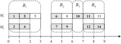
Example 1 Consider an instance of the problemP|rj,pj =

1|F(C,w)withm =2 machines,n =14 jobs and a

non-decreasing objective functionFof job completion times. For

the release dates presented in the table

j 1 2 3 4 5 6 7 8 9 10 11 12 13 14

rj 0 0 1 1 0 4 4 4 5 6 7 7 7 8

the Algorithm ‘Calculate Blocks’ finds the block sets

B1 = {1,2,3,4,5},B2 = {6,7,8,9},B3 = {10},B4 =

{11,12,13,14}and their starting timest1=0,t2=4,t3= 6,t4=7. The corresponding setsTjareT1= {0,1,2},T2=

{4,5},T3 = {6},T4 = {7,8}and the number of jobsh(t) scheduled in[t,t+1[is

t 0 1 2 3 4 5 6 7 8

h(t) 2 2 1 − 2 2 1 2 2

A feasible earliest start schedule C with block sets

B1,B2,B3and B4is shown in Fig.1. The jobs which start exactly at their release dates are dashed; the remaining jobs start after their release dates.

If a scheduleCis given by a list of unit time intervals and a list of jobs allocated to them, then conditions (i)–(iii) can

Fig. 1 The Gantt chart of scheduleCfound by Algorithm ‘Calculate

[image:3.595.310.541.604.689.2]

(4)

be verified for all time slots inO(n)time by scanning the

time slots ofCthree times.

In the first scan, the algorithm identifies time-values τ1, τ2, . . . , τkwith the property: all jobs that start atτu,1≤

u≤k, have their release times equal toτu. Clearly, the

iden-tifiedτ values satisfy property (i) of the block definition, and therefore they get a label of a ‘t-candidate.’

In the second scan, the algorithm removes from the list

of ‘t-candidates’ those values which do not satisfy property

(ii): a ‘t-candidate’ τu cannot define the starting time of a

block if there is a job j starting after τu (Sj > τu) which

is related to an earlier block (rj < τu). To check condition

(ii) efficiently, the ‘t-candidates’ are scanned right to left

updatingρaccordingly.

The third scan is performed to verify property (iii) for the remaining ‘t-candidates.’

The formal description of this approach is presented in Appendix 1 as Algorithm ‘Earliest Start Schedule Verifica-tion.’ Its time complexity isO(n): there are no more thann

unit time slots and they are scanned three times. The first two

scans each considernvalues ofrj; the third scan counts the

number of jobs assigned to each time slot, which total

num-ber isn. Notice that as a by-product, the algorithm returns

thet values, which define the decomposition of an earliest

start schedule into the blocks.

2.2 Transforming an arbitrary schedule into an earliest start schedule

In this section we show that if a given scheduleCfor problem

P|rj,pj =1|Fdoes not belong to the class of earliest start

schedules, it can be transformed into an earliest start schedule

Cwithout increasing any of the completion times:

C_j ≤Cj for all j∈ J. (1)

This can be achieved as follows. Algorithm ‘Calculate Blocks’ is applied first in order to define the structure of the

earliest start schedule, namely the time intervalsT and the

number of jobs allocated to themh(t),t ∈T. Time intervals

[t,t +1[,t ∈ T, are considered one by one, starting with the earliest one. All jobs allocated in the original schedule to those time intervals are kept. If their number is less than

h(t), the required number of additional jobs is moved from

later time intervals to[t,t+1[; the preference is given to the jobs with the smallest release dates. The formal

descrip-tion of such an algorithm (entitled as ‘Left Shift(C)’) and

its analysis are presented in Appendix 1. We also discuss

implementation details which result in theO(nlogn)time

complexity.

The following proposition establishes a link between a given optimal schedule and the earliest start optimal sched-ule.

Proposition 1 A scheduleCis optimal for problem P|rj,pj

=1|F(C,w)with a non-decreasing objective function F , if and only if it can be transformed by Algorithm ‘Left Shift(C)’ into an optimal earliest start scheduleC = C₁, . . . ,Cn

without changing the value of the objective function.

Proof Due to the properties of Algorithm ‘Left Shift(C),’ schedulesCandCsatisfy inequalities (1). This implies that

for a non-decreasing objective functionF,

FC,w≤F(C,w) . (2)

IfCis optimal, then condition (2) should hold as equality

since a strict inequality contradicts optimality ofC. On the

other hand, ifCcan be transformed into an optimal earliest

start schedule C without changing the objective function

value, then clearlyCmust be optimal.

Due to the described relationship between an arbitrary

schedule Cand an earliest start schedule C, in the

subse-quent sections we deal with earliest start schedules only. The optimality conditions which we formulate can be applied to each block separately, since no job from a block can be moved to a previous block.

Notice that if a given schedule does not belong to the class of earliest start schedules, then one can first apply Algo-rithm ‘Left Shift(C)’ checking condition (2) for the resulting scheduleC. IfFC,w<F(C,w), then scheduleC

can-not be optimal; ifFC,w = F(C,w)then one needs to

verify the optimality of the earliest start scheduleCapplying the necessary and sufficient conditions to it.

2.3 Earliest start schedule and associated compressed network

Consider problem P|rj,pj =1|F(C,w)with a separable

objective function F =wj fj(Cj), where each function

fj(Cj)is non-decreasing. For a given earliest start

sched-uleCconsisting of a single block, the total number of time

intervals is

ν= n

m

,

so thatT = {0,1, . . . , ν−1}, and for each timet ∈T there are exactlyh(t)jobs allocated to[t,t+1[:

h(t)=

m, 0≤t ≤ν−2,

n−m(ν−1)≤m,t=ν−1.

(5)

the cost of delivering the flow. This implies that the necessary and sufficient conditions of optimality of a given schedule are equivalent to non-existence of a negative cycle in the corre-sponding residual network.

Formally, the transportation problem is defined by net-workN(C)=(V,A(C), η),

V = {1, . . . ,n} ∪ {It|t ∈T},

A(C)= {(j,It) | jis assigned or can be assigned toIt}.

Here, the vertex setV consists of job nodes{1, . . . ,n}, each

of which has a supply of 1, and interval nodes{It |t ∈T}

with demandh(t). The arc setA(C)consists of the arcs(j,It)

defined for each feasible allocation of jobjto interval[t,t+

1[,t ≥ rj. The cost of an arc(j,It)represents the cost of

allocating job jto time interval[t,t+1[:

ηj t =wj × fj(t+1)

and its capacity is 1. Depending on the type of the objective function,

ηj t = ⎧ ⎨ ⎩

wj ×(t+1), if F =

wjCj,

wj ×Uj(t+1) , if F =

wjUj,

wj ×Tj(t+1) , if F =

wjTj.

For a given solution C, a residual network Nr(C) =

(V,Ar(C), ξ)has the same vertex set V, while the arc set

Ar(C)and the costsξ are defined as follows:

Ar(C)= {(It,j) | j is allocated inCto[t,t+1[}

∪(j,It)| jis not allocated inCto[t,t+1[,t ≥rj

; ξt j = −wj × fj(t+1)for arcs (It,j) ,

ξj t =wj× fj(t+1)for arcs (j,It) .

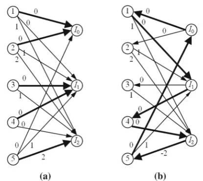
Example 2 Consider problemP|rj,pj = 1|

wjTj with

m=2 machines andn=5 jobs with release dates, due dates

and weights presented in the table:

j 1 2 3 4 5

rj 0 0 1 1 0

dj 2 1 2 3 1

wj 1 1 1 1 1

Observe that the release dates are the same as those of the

first 5 jobs of Example1processed as one block. The

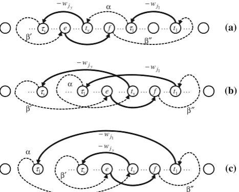
trans-portation networkN(C)is shown in Fig.2a and the residual

network corresponding to the schedule given by the first

block of Fig.1is presented in Fig.2b. The numbers at the

[image:5.595.320.528.53.238.2]

arcs indicate the arc costs.

Fig. 2 a Network N(C)for jobs {1,2,3,4,5}of Example 2 and

bresidual networkNr₍_C₎_{for the schedule given by block}_B

1of Fig.1

Reformulating the well-known network flow theorem

(see, e.g., Ahuja et al. 1993) we conclude that an

earli-est start schedule C is optimal for problem P|rj,pj =

1|wj fj(Cj)if and only if the corresponding residual

net-workNr(C)=(V,Ar(C), ξ)constructed for each block of

Ccontains no negative cycle.

A cycle in the residual network Nr(C) is of the form

It1,j1,It2,j2, . . . ,Itκ,jκ,It1. The arcs are alternating

between an arc from an interval node It to a job node j

and from a job node to an interval node.

It is convenient to compress the residual network Nr(C)

into a networkN(C)by eliminating the job nodes; this results in multiple arcs connecting the interval nodes. We denote the nodes inN(C)byt ∈ {0,1, . . . , ν−1}. For any two nodest

andtwe have an arc fromttotwith lengthξt j+ξj t, where

ξt j+ξj tis the change of the objective function

wjfj(Cj)

when job jis moved from[t,t+1[to[t,t+1[. Such an arc

replaces the two alternating arcs It → j → It inNr(C).

It is important to notice that the length₍t,t)of the arc from

t tot depends not only ont andt, but on job j allocated

inCto[t,t+1[. Since there areh(t)jobs allocated to each time interval, there areh(t)arcs(t,t)fort >t since any job allocated to[t,t+1[can be moved to a later time slot

[t,t+1[. However, fort <t there can be less thanh(t)

arcs since not every job allocated to[t,t+1[can be moved to an earlier time slot[t,t+1[.

For the three objective functions we consider, the cost of the arc(t,t), associated with job jallocated to[t,t+1[, is given by

(t,t)= ⎧ ⎨ ⎩

wj×(t−t), if F=wjCj;

wj×Ujt+1−Uj(t+1), if F=wjUj;

wj×

Tj

t+1−Tj(t+1)

(6)

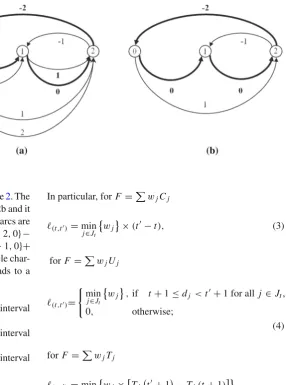
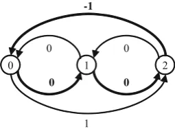
Fig. 3 Two compressed networks for Example2:

aN(C)andbN(C)

Example 3 Consider again the instance from Example2. The

corresponding residual network is presented in Fig.2b and it

contains a negative cycleI0, 1, I1, 4, I2,5, I0(its arcs are in bold) of length−w1max{1−2,0}+w1max{2−2,0}− w4max{2−3,0}+w4max{3−3,0}−w5max{3−1,0}+ w5max{1−1,0} = −2w5= −2. This negative cycle char-acterizes that the series of the following moves leads to a

schedule with a smaller value ofwjTj:

– moving job 1 from time interval [0,1[to time interval

[1,2[,

[2,3[,

[0,1[.

The compressed residual network is shown in Fig.3a, and

the corresponding negative cycle (marked by bold arcs) is 0,1,2,0.

We distinguish between right and left arcs inN(C). Arc

(t,t)is aleft arcif it is directed fromt to a vertex corre-sponding to an earlier time slott,t < t; for a right arc

(t,t),t>t.

Consider a pair of time-nodest andt, corresponding to

time intervals[t,t +1[ and[t,t +1[. Since our aim is to detect negative cycles or to prove that none exists, we

can compress networkN(C)further by eliminating multiple

arcs of larger costs. Instead of keeping multiple arcs(t,t)

and multiple arcs(t,t), we can keep just one arc in each

direction that has the smallest cost.

Denote the resulting network by N(C). For Example 2,

the corresponding networkN(C)is shown in Fig.3b. LetJt

be the set of jobs assigned inCto time interval[t,t +1[. Then the cost (or the length) of the right arc(t,t),t < t,

originating fromtis defined as

(t,t)=min j∈Jt

wj×

fj

t+1− fj(t+1)

.

In particular, forF=wjCj

₍t,t)=min j∈Jt

wj

×(t−t), (3)

forF =wjUj

(t,t)=

min

j∈Jt

wj

,if t+1≤dj <t+1 for all j ∈ Jt,

0, otherwise;

(4)

forF =wjTj

(t,t)=min j∈Jt

wj ×

Tj

t+1−Tj(t+1)

.

Considering left arcs (t,t),t > t, originating fromt, we need to take into account the release dates of the jobs

from Jt since not all of them can be moved to an earlier

time slot[t,t+1[. LetJ₍t,t)denote a subset of jobs from

Jt, which can be re-allocated to[t,t+1[without violating

their release dates:

J₍t,t) =

j ∈ Jt|rj ≤t

.

Then the left arct,texists if J₍t,t) = ∅and its length is

defined as

(t,t)= − max j_∈J₍_t_,_t₎

wj

fj(t+1)− fj

t+1.

In particular, forF=wjCj

(t,t)= − max j∈J₍_t_,_t₎

wj

[image:6.595.259.546.53.439.2]

(7)

forF=wjUj

(t,t)= ⎧ ⎪ ⎪ ⎨ ⎪ ⎪ ⎩

0, ift+1>djort+1≤dj

for allj∈J₍t,t),

−max j∈J₍t,t), t+1≤dj<t+1

wj

, otherwise;

forF=wjTj

(t,t)= − max j∈J₍_t_,_t₎

wj

Tj(t+1)−Tj

t+1.

It is easy to make sure that if residual network Nr(C)

and the corresponding compressed networkN(C)contain a

negative cycle with repeated nodet, then the cycle can be

decomposed into two cycles and at least one of them is neg-ative. Clearly, it is sufficient to consider the cycles without repeated time-values. Thus the necessary and sufficient opti-mality conditions can be formulated as follows.

Theorem 1 A scheduleCfor a given instance of P|rj,pj =

1|wjfj(Cj)is optimal if and only if

1. transformingCinto an earliest start schedule does not change the objective value;

2. for each block of the resulting earliest start schedule, the corresponding compressed network N(C)contains no negative cycle.

We estimate the size of the compressed networkN(C)and

the time complexity of constructing it assuming that a given

earliest start scheduleChasnjobs assigned tommachines

and it consists of a single block. The number of nodes of

N(C)isν=_mn. Each pair of nodestandtare connected by at most two arcs(t,t)and(t,t), so that the total number of arcs isOν2. For each right arc(t,t), its cost can be

found inO(m)time since |Jt| ≤ m, and for each left arc

(t,t), its cost can also be found inO(m)time since|J₍t,t)| ≤

m. Thus the overall time complexity of constructingN(C)is

Omν2=O

n2

m

.

In the subsequent sections we show that, depending on

the type of the problem, Condition 2 of Theorem1can be

reformulated so that instead of checking the non-negative condition for all possible cycles only special types of cycles can be considered, namely two-node cycles, chain cycles and spiral cycles. Each of these cycles has exactly one arc of negative length denoted by(t, τ); it originates in the

right-most node t of the cycle and contains no more than one

positive arc; all other arcs have zero lengths. If the cycle

contains a positive arc, that arc has end-nodet.

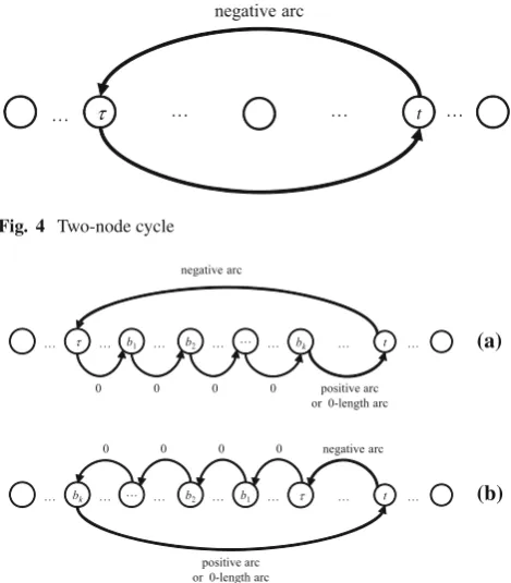
Atwo-node cycleconsists of two arcs(t, τ)and(τ,t), see Fig.4.

Achain cycleconsists of an arc in one direction and a

chain of arcs in the opposite direction. Aright-chain cycle

t τ

negative arc

…

… …

…

Fig. 4 Two-node cycle

(a)

(b)

Fig. 5 Chain cycles:aright-chain cycle andbleft-chain cycle

starts with the negative left arc(t, τ)and then proceeds with a chainRof right arcs fromτ tot, see Fig.5a. Aleft-chain cyclestarts with the negative left arc(t, τ), proceeds then

with a chainLof left arcs to the left-most node of the cycle

and returns to the origintvia one right arc, see Fig.5b. Aspiral cycleis defined as the one satisfying the following five properties.

Property 1: The cycle contains exactly one negative arc (t, τ), all other left arcs have zero length.

Property 2: No left arc, except for possibly(t, τ), spans over a node which appears in the remaining part of the cycle after that arc.

Property 3: No right arc spans over a node which appears in the remaining part of the cycle after that arc.

Property 4: The right-most node of the cycle ist.

Property 5: All right arcs have zero length except for the

last right arc terminating int which may be of positive

length or of zero length.

An example of a spiral cycle is shown in Fig.6. In general, a spiral cycle contains alternating left chainsL1,L2, . . . ,Ls

and right chainsR1,R2, . . . ,Rs: the negative left arc(t, τ)

is followed byL1,R1,L2,R2, . . . ,Ls,Rs terminating int,

see Fig.6.L1is a left chain originating inτ; the first arc of

R1spans over all nodes ofL1; the first arc ofL2spans over all nodes ofL1∪R1. For eachk =2, . . . ,s, the first arc of

[image:7.595.307.542.56.324.2]

(8)

… …

τ

… …

… … t …

negative arc

positive arc or 0-length

arc 0

0

0 …

… … … …

0 0

0

0 0

0

L2

R1

R2

L1

[image:8.595.84.512.53.249.2]

Fig. 6 Spiral cycle

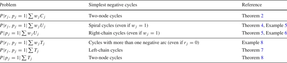
Table 1 The simplest cycles which are sufficient to consider in optimality conditions

Problem Simplest negative cycles Reference

P|rj,pj=1|wjCj Two-node cycles Theorem2

P|rj,pj=1|wjUj Spiral cycles (even ifwj=1) Theorem4, Example5

P|pj=1|wjUj Right-chain cycles (even ifwj=1) Theorem5, Example6

P|rj,pj=1|wjTj Cycles with more than one negative arc (even ifrj=0) Example8

P|rj,pj=1|Tj Left-chain cycles Theorem7

P|pj=1|Tj Two-node cycles Theorem8

and the first arc ofRkspans over all nodes ofL1,R1,L2,R2, …,Lk−1,Rk−1,Lk. The last chainRs consists of right arcs

terminating in the origint.

Notice that a two-node cycle is a special case of a chain cycle, which in its turn is a special case of a spiral cycle.

The main outcomes of our study are summarized in

Table1, where we list the types of cycles that should be

examined in a compressed residual network N(C),

repre-senting a one-block earliest start schedule. Notice that for problemP|rj,pj =1|

wjTjand its special caseP|pj =

1|wjTjthere exist instances for which even the simplest

negative cycles have several negative arcs so that they do not fall in any of the above three categories of cycles. We do not give a characterization of negative cycles for these two problems since the usage of such a result is likely to be very limited. For example, using those conditions in the optimal-ity check would incur cycles with one negative arc, cycles with pairs of negative arcs and even more complex cycles with various combinations of negative arcs.

For all other problems and their special cases, we first prove the result establishing the type of a simplest negative cycle. Then we show that the result cannot be improved by providing an example that there exists an instance of the

problem with only one negative cycle and it is of the type established in the corresponding theorem. Such instances are not needed for two-node cycles indeed.

In what follows we consider the three objective functions

wjCj,wjUj andTj and prove the relevant

state-ment about the type of the cycle for each problem. We then explore how the identified types of cycles can be used in order to speed up the optimality check.

3 Problem

P

|

r

j

,

p

j

=

1 |

w

j

C

j

In this section we consider the problem P|rj,pj =

1|wjCjwith the weighted completion time objective. We

show that the optimality conditions for this problem can be simplified by limiting consideration to two-node cycles only.

Moreover, the reduced network N(C)can be compressed

further by eliminating transitive arcs, so that the resulting net-workNTransRem(C)contains no more than 2(ν−1)arcs; its left arcs form an out-tree and the right arcs form an in-tree. As

a result, the optimality check problem can be solved inO(n)

time, an improvement in comparison with the O(nlogn)

[image:8.595.52.544.296.404.2]

(9)

Theorem 2 A compressed residual network N(C), repre-senting a one-block earliest start schedule for a given instance of problem P|rj,pj =1|

wjCj, contains a

neg-ative cycle if and only if it contains a negneg-ative two-node cycle.

Proof Clearly, the formulated condition is sufficient. In order to prove that it is also necessary, assume that there exists an instance of problem P|rj,pj = 1|

wjCj such that all

two-node cycles are non-negative while there exists a nega-tive cycle with three or more nodes. Let this cycle additionally have the smallest number of nodes. We show that there exists a negative cycle with a smaller number of nodes.

Denote byt1the left-most node of the cycle. The cycle

starts with a positive arc(t1,t2), proceeds with a series of

arcs, which we denote byα, leading to nodet3and terminates

at the origint1with a negative arc(t3,t1). The length of the positive arc(t1,t2)iswj1(t2−t1), where job j1is selected in accordance with (3) so that

wj1 =min

j∈Jt₁

wj

;

the length of the negative arc(t3,t1)is−wj3(t3−t1), where job j3is selected in accordance with (5) so that

wj3 = max

j∈J₍_t_3,_t₁₎

wj

. (6)

Thus the length of the original cycle is

=wj1(t2−t1)+α−wj3(t3−t1), (7)

where_αis the length of fragmentα.

First we derive an auxiliary inequality forwj1 andwj3. Due to the assumption, the cycle consisting of two arcs (t3,t1)and(t1,t3)is non-negative. Since its length is(−wj3+ wj1)(t3−t1), we conclude that

−wj3+wj1 ≥0. (8)

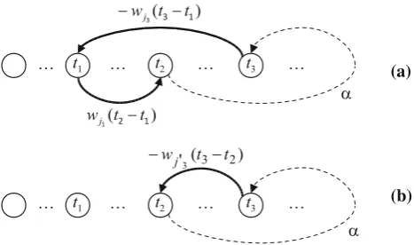
Consider the following two cases, depending on the loca-tion oft2andt3. Ift2 <t3, cycle((t1,t2) , α, (t3,t1))is of the form shown in Fig.7a. Since there exists arc(t3,t1)in

N(C), the set of jobsJ₍t3,t1), which can be re-allocated from [t3,t3+1[to[t1,t1+1[is non-empty, and therefore the set

J₍t_3,t₂₎ is also non-empty fort2 > t1. Hence we can intro-duce the arc(t3,t2)and consider a cycle with less nodes, namely(α, (t3,t2)), see Fig. 7b. The length of (t3,t2) is

associated with some job j₃, wj₃ = max

j∈J₍t3,t₂)

wj

, and due

toJ₍t3,t2) ⊇J(t3,t1),

wj₃ ≥wj3. (9)

(a)

(b)

Fig. 7 Replacing negative cycle((t1,t2) , α, (t3,t1))by(α, (t3,t2))if

t1<t2<t3

Comparing the length of the original cyclegiven by (7)

with the length of the new cycle=_α −wj₃(t3−t2)we

conclude that if <0, the new cycle is also negative:

₋₌_α₋_w

j₃(t3−t2)

−wj1(t2−t1)+α−wj3(t3−t1)

≤ −wj3(t3−t2)−

wj1(t2−t1)−wj3(t3−t1)

=wj3−wj1

(t2−t1)≤0.

In the above formula, the first inequality is due to (9),

while the second inequality follows from (8). Thus we have

detected a negative cycle with a less number of nodes which contradicts the assumption that the initial negative cycle has the smallest number of nodes.

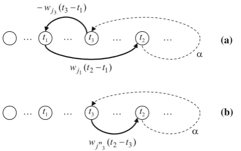
If t2 > t3, as shown in Fig. 8a, introduce the positive

arc (t3,t2) and consider a cycle with less nodes, namely

((t3,t2) , α), see Fig. 8b. The length of(t3,t2)is associated with some job j₃, wj₃= min

j∈Jt₃

wj

, see (3). Comparing the

latter formula with (6) we conclude that

wj₃ = min j∈Jt3

wj

≤ min

j∈J₍t3,t1)

wj

≤ max

j∈J₍t3,t1)

wj

=wj3

(10)

(notice thatJt3 ⊇J(t3,t1)and the last equality corresponds to (6)).

Denoting bythe length of the cycle shown in Fig. 8b,

we obtain

−=wj₃(t2−t3)+α

−wj1(t2−t1)+α−wj3(t3−t1)

≤wj3(t2−t3)−

wj1(t2−t1)−wj3(t3−t1)

=wj3−wj1

(t2−t1)≤0,

so that < 0 for < 0. In the above formula, the first

[image:9.595.308.542.54.192.2]

(10)

(a)

(b)

Fig. 8 Replacing negative cycle((t1,t2) , α, (t3,t1))by((t3,t2) , α)if

t1<t3<t2

from (8). Again we have detected a negative cycle with a less

number of nodes which contradicts the assumption that the initial negative cycle has the smallest number of nodes.

Notice that due to the definition ofN(C), a right arc exists

for any pair of nodes, while left arc (t, τ) exists only if

J₍t,τ) = ∅. Therefore in order to enumerate all two-node

cycles one can consider left arcs one by one, complement-ing each left arc with its right arc counterpart. Moreover, we prove that transitive left arcs inN(C)are not needed.

Theorem 3 Consider network NTransRem(C)obtained from

N(C)by removing transitive left arcs and removing all right arcs which do not have a left counterpart. Denote the set of left arcs in NTransRem(C)by Aleft(C). Then N(C)does not

contain a negative cycle if and only if inequality

min

j∈J_τ

wj

≥ max

j∈J₍t,τ)

wj

. (11)

is satisfied for each(t, τ)∈ Aleft(C), τ <t .

Proof NecessityClearly, relation (11) formulated for a left arc(t, τ)is an equivalent representation of the condition that

the cycle defined by nodestandτ is non–negative, see

for-mulae (3) and (5).

SufficiencyTo prove that conditions (11) defined for(t, τ)∈ Aleft(C), are sufficient, consider t1 < t2 < t3 assum-ing that the left arcs(t2,t1) , (t3,t2)exist together with the transitive left arc(t3,t1). The associated positive arcs are (t1,t2) , (t2,t3)and(t1,t3). We show that if (11) holds for the pair of nodest1,t2and for the pairt2,t3, then (11) also holds for the pair of nodest1,t3.

Indeed, conditions (11) fort1,t2and fort2,t3are of the form:

min

j∈Jt₁

wj

≥ max

j∈J₍_t_2,_t₁₎

wj

,

min

j∈Jt₂

wj

≥ max

j∈J₍t3,t2)

wj

.

The right-hand side of the first inequality is greater than or equal to the left-hand side of the second inequality since

J₍t2,t1)⊆Jt2:

max

j_∈J₍_t_2,_t₁₎

wj

≥ min

j_∈J₍_t_2,_t₁₎

wj

≥ min

j_∈Jt2

wj

.

The right-hand side of the second inequality can be bounded as

max

j_∈J₍_t_3,_t₂₎

wj

≥ max

j_∈J₍_t_3,_t₁₎

wj

sinceJ₍t_3,t₂₎⊇ J₍t3,t1). We conclude that

min

j∈Jt₁

wj

≥ max

j∈J₍t3,t1)

wj

,

which implies that condition (11) also holds for the pair of

nodest1,t3.

Proposition 2 The set of left arcs Aleft(C)in NTransRem(C)

is an out-tree.

Proof Suppose the proposition does not hold, i.e., there exists inAleft(C)a pair of left arcs(t2,t1)and(t3,t1)with the same end-node,t1 < t2 < t3. This implies that J₍t_2,t₁₎ = ∅and

J₍t3,t1)= ∅. It follows from the latter condition thatJ(t3,t2)= ∅ since the jobs that can be re-allocated from [t3,t3+1[ to[t1,t1+1[can also be re-allocated to[t2,t2+1[. Then there exists arc(t3,t2)inN(C)and therefore the set of arcs

Aleft(C)in network NTransRem(C)(without transitive arcs) cannot contain(t3,t1), a contradiction.

Example 4 The following table describes an instance of

problemP|rj,pj =1|wjCjwithn =18 jobs andm=2

machines:

j 1 2 3 4 5 6 7 8 9 10 11 12 13 14 15 16 17 18

rj 0 0 0 0 2 2 3 1 3 2 5 5 5 4 7 5 6 7

C_j 1 1 2 2 3 3 4 4 5 5 6 6 7 7 8 8 9 9

A feasible scheduleCfor this problem is shown in Fig.9.

The jobs which start exactly at their release dates are dashed; the remaining jobs start after their release dates.

The left arcsAleft(C)of graphNTransRem(C)with transi-tive arcs removed are shown in Fig.10. The setAleft(C) con-sists of (8,7) , (7,6) , (6,5) , (6,4) , (4,3) , (3,2) , (3,1) , (1,0), which form an out-tree.

The proof of Proposition2justifies the followingO(n)

[image:10.595.55.290.53.200.2]

(11)

Fig. 9 Gantt chart of a feasible scheduleCof Example 4

Fig. 10 Left arcsAleft(C)of graph NTransRem(C)without transitive

arcs for a feasible scheduleCof Example4

NTransRem(C)without transitive arcs. It first connects consec-utive nodes into left chains and then defines for the right-most node of each chain an arc ending in that node with the origin in the subsequent chain, giving preference to the left-most possible origin. Having constructed the set Aleft(C)of left arcs, the corresponding right arcs can be produced also in

O(n)time. Since|Aleft(C)| = ν−1, there areν−1

two-node cycles, which can be enumerated inO(ν)time, so that

the overall time complexity of the optimality check isO(n). We provide the details of this approach in Appendix 2.

4 Problem

P|r

j

,

p

j

=

1 |

w

j

U

j

This section explores the most general, spiral cycles.

Theorem 4 A compressed residual network N(C), repre-senting a one-block earliest start schedule for problem P|rj,pj = 1|

wjUj, contains a negative cycle if and

only if it contains a negative spiral cycle.

Proof Consider an arbitrary negative cycle that starts with a negative arc(t, τ). We show that then there exists a negative cycle such that the five properties formulated in the definition of a spiral cycle are satisfied.

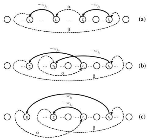
In order to prove Property 1 (the cycle contains exactly one negative arc(t, τ)) we demonstrate that a negative cycle with the smallest number of nodes cannot contain more than one negative arc. Suppose a negative cycle has several neg-ative arcs(t1, τ1), (t2, τ2), . . . , (ty, τy),y≥2. Without loss

of generality we assume that arc(t1, τ1)has the right-most origint1among all negative arcs, i.e.,t1>max

t2, . . . ,ty

. Notice that no nodes are repeated in the cycle. Denoting the path fromτ1toty byαand the path fromτy tot1byβ, the cycle can be represented in the form(t1, τ1) , α,

ty, τy

, β,

where fragmentαcan be empty. The three possible types of

that cycle are illustrated in Fig.11a–c depending on the rela-tionship betweenτ1,tyandτy. Let the lengths of arcs(t1, τ1) andty, τy

be−wj1and−wjy, where j1andjyare late jobs

allocated to[t1,t1+1[and[ty,ty+1[, respectively.

… ty τ1 … … t1

… _τy … … _(a)

α

β

… t1

τ1 … ty …

… _τy … … …

1

j

w − y

j

w −

α

1

j

w − y

j

w

−

(b)

… t1

τ1 … τy … ty … … … (c)

1

j

w

−

α

β

β y

j

w

[image:11.595.302.543.54.282.2]

−

Fig. 11 Negative cycle(t1, τ1) , α,

ty, τy

, β

Since the cycle passes throughtybefore it returns tot1and

ty <t1, there should be an arc(e, f)belonging to fragment

βthat straddles nodety, so that

e<ty < f,

and we can represent fragment β as β, (e,f) , β, see

Fig.12. Notice that the casee=τy impliesβ = ∅and the

case f =t1 impliesβ = ∅. Let the job corresponding to

arc(e,f)beqso that the length of the arc is

(e,f)=

wq, if e<dq ≤ f,

0, otherwise. (12)

Since fragment β does not contain negative arcs, all its

three components are non-negative:

β ≥0, (e,f)≥0,

β ≥0.

Here_β, (e,f)and_βdenote the lengths ofβ, (e, f) , β,

respectively.

Consider instead of the original cycle two new cycles:

C ycleI = ty, τy

, β_,_e_,_t_y _and_{C ycle}_{I I} ₌₍₍_t₁_{, τ}₁_{) ,} α,ty, f

, β_{. Notice that}

(e,ty) ≤(e,f)

sincety< f. Moreover

(12)

… f t1

τ1 … τy e … ty … … … (c)

1

j

w −

y j

w − α

… ty f … τ1 … … t1

… _τy … e … … _(a)

1

j

w − y

j

w

− _α

… f t₁

τ1 … ty …

… _τy … e … … _(b)

1

j

w − y

j

w −

α

β′ _{β ′′}

β′

β ′′

Fig. 12 Negative cycle with fragment β decomposed into

β_{, (}_e_,_f_{) , β}

sinceJtycontains a late job (it defines the cost of the negative

left arc(ty, τy)). Thus we have

(e,ty)+(ty,f)≤(e,f).

Denoting the length of the original cycle by O and the

lengths of the two new cycles byI andI I we obtain:

I +I I ≤O <0. (13)

Thus at least one of the new cycles is negative. This contra-dicts the assumption that the initial negative cycle has the smallest number of nodes.

We turn now to Property 2: no left arc, except for possibly

(t, τ), spans over a node which appears in the remaining

part of the cycle after that arc. Suppose for a negative cycle satisfying Property 1 there exists a 0-length left arc(f,g)

which spans over nodeh that appears on the path fromgto

t, so thatg<h< f, see Fig.13. If there are several nodes

of typeh we select the right-most one. In that figure, solid

lines represent arcs and dotted lines represent the fragments of the cycle which may consists of several arcs. Introduce new left arc(f,h), which length is zero since there is only

one negative left arc(t, τ). Replacing the fragment of the

cycle from f tohby the arc(f,h), we remove 0-length left arcs and non-negative right arcs. Hence the resulting cycle is negative, but with less left arcs spanning over other nodes

on the path tot. Repeating this transformation we eventually

obtain a cycle satisfying Property 2.

The proof of Property 3 (no right arc spans over a node which appears in the remaining part of the cycle after that arc) is similar to the proof of Property 2: consider a right arc

(f,g)which spans over nodehthat appears on the path from

…

h … f … τ

…

g

… … _t …

negative arc

positive arc or 0-length arc 0

0 0

[image:12.595.54.288.58.246.2]

0 0

Fig. 13 Negative cycle with left arc(f,g)spanning over nodehon

the path fromgtot

gtot, so that f <h <g, and replace the fragment of the cycle from f tohby the arc(f,h)with₍f,h)≤(f,g).

The same idea can be used to prove Property 4 (t is the

right-most node of the cycle) usingtinstead ofhin the above

arguments.

Finally, consider Property 5: all right arcs have zero length

except for the last right arc terminating intwhich may be of

positive length or of zero length. Let there exists a negative cycle satisfying Properties 1–4, but not satisfying Property 5. Let the origin of the negative arc betand let the first positive

arc be (e, f), where f < t due to Property 4. Again we

introduce a new arc(e,t). For the positive arc(e, f)all jobs

from Je are early and they become late if re-allocated to

[f,f +1[, (e,f) = minj∈Je{wj}, see (4). Then the same

holds for(e,t), which implies

(e,t)=min j∈Je

{wj} =(e,f).

Thus replacing the fragment frometotby arc(e,t)results in a negative cycle with less nodes and no more than one positive arc(e,t).

Clearly, spiral cycles have a more complex structure in comparison with two-node cycles and chain cycles. We

demonstrate by means of Example5below that the result of

Theorem4cannot be strengthened for problem P|rj,pj =

1|wjUj, and spiral cycles cannot be replaced by simpler

counterparts. Since the instance below deals with the case of

unit weights,wj =1 for all j ∈ J, the result of Theorem4

cannot be strengthened for problem P|rj,pj =1|

Uj.

Example 5 Consider an instance of the problemP|rj,pj =

1|Ujfor which a negative spiral cycle exists but there are

no negative cycles of simpler types. In that example, there is

one machine andn = 8 jobs with job characteristics given

by the table:

j 1 2 3 4 5 6 7 8

rj 0 1 2 2 1 0 6 3

dj 7 6 5 4 5 6 8 4

(13)

7

3 4

1 2 5 6

0

0 -1

0 0 0 0 0

[image:13.595.361.489.56.150.2]

0

Fig. 14 A unique negative cycle for Example5belonging to the spiral

5 Problem

P

|

p

j

=

1 |

w

j

U

j

We consider now the special case when all jobs are available

simultaneously (rj = 0 for j ∈ J) and show that for this

case it is sufficient to consider simpler cycles of chain type.

Theorem 5 A compressed residual network N(C), repre-senting a one-block earliest start schedule for problem P|pj =1|

wjUj, contains a negative cycle if and only if

it contains a negative right-chain cycle.

Proof Since problemP|pj =1|wjUjis a special case of

P|rj,pj =1|

wjUj, we can use the result of Theorem4

and consider only negative spiral cycles. Letzbe the

left-most node of such a cycle. Consider a negative arc(t, τ)of

the cycle, which corresponds to moving some job j ∈ J₍t,τ)

to time interval[τ, τ +1[. Since all release dates are zero,

arc(t, τ) can be replaced by arc(t,z)which corresponds

to moving the same job j to time interval [z,z+1[, the

1 2

0

-1

0 0

[image:13.595.53.291.56.179.2]

1

Fig. 15 A unique negative cycle for Example6belonging to the

right-chain category

length of the new arc being no larger than that of(t, τ). Since

the remaining part of the spiral cycle fromztot is a right

chain with 0-length arcs except for the last arc, which can be positive, the new cycle with the shortcut(t,z)is a right-chain cyclet,z, . . . ,tof negative length.

The result formulated in Theorem5cannot be

strength-ened for the unweighted version P|pj = 1|

Uj, as the

following example illustrates.

Example 6 Consider an instance of the problem P|pj =

1|Ujwith one machine and three jobs with due datesd1=

2,d2 = 3,d3 = 1, and a schedule given by job sequence

(1,2,3). The corresponding graph, shown in Fig.15, con-tains a unique negative cycle(2,0,1,2)of length−1; it is a right-chain cycle; all two-node cycles are non-negative.

In what follows we show that network N(C) can be

reduced by removing some nodes and arcs. Recall that the

network reduction has been performed in Sect. 3for

prob-lem P|rj,pj = 1|

wjCj where it has been shown that

transitive arcs are not needed.

We start with decomposing N(C) into so called

zero-components. A zer o-component Zi,1 ≤ i ≤ γ, consists

of consecutive nodesτ_i, τ_i +1, . . . , τi, each of which can

be reached from the start-nodeτivia a chain of 0-length right

arcs. For two zero-componentsZi andZj,i < j, there is no

0-length right arc(τ, τ)connectingτ ∈ Zi andτ ∈ Zj.