Optimized hybrid localisation with cooperation in wireless sensor networks

White Rose Research Online URL for this paper:

http://eprints.whiterose.ac.uk/117181/

Version: Publishers draft (with formatting)

Article:

Khan, MW, Kemp, AH and Salman, N (2017) Optimized hybrid localisation with

cooperation in wireless sensor networks. IET Signal Processing, 11 (3). pp. 341-348. ISSN

1751-9675

https://doi.org/10.1049/iet-spr.2015.0390

© The Institution of Engineering and Technology. This paper is a postprint of a paper

submitted to and accepted for publication in IET Signal Processing and is subject to

Institution of Engineering and Technology Copyright. The copy of record is available at the

IET Digital Library.

[email protected] https://eprints.whiterose.ac.uk/ Reuse

Unless indicated otherwise, fulltext items are protected by copyright with all rights reserved. The copyright exception in section 29 of the Copyright, Designs and Patents Act 1988 allows the making of a single copy solely for the purpose of non-commercial research or private study within the limits of fair dealing. The publisher or other rights-holder may allow further reproduction and re-use of this version - refer to the White Rose Research Online record for this item. Where records identify the publisher as the copyright holder, users can verify any specific terms of use on the publisher’s website.

Takedown

If you consider content in White Rose Research Online to be in breach of UK law, please notify us by

Optimised hybrid localisation with cooperation in wireless sensor networks

M. W. Khan∗, Naveed Salman, A. H. Kemp.

School of Electronic and Electrical Engineering, University of Leeds, United Kingdom.

∗_{corresponding author: [email protected]}

Abstract

In this paper we introduce a novel hybrid cooperative localisation scheme when both distance and angle measurements are available. Two linear least squares (LLS) hybrid cooperative schemes based on angle of arrival-time of arrival (AoA-ToA) and AoA-received signal strength (AoA-RSS) signals are proposed. The proposed algorithms are modified to accommodate cooperative localisation in resource constrained networks where only distance measurements are available between target sensors (TSs) while both distance and angle measurements are available between reference sensors (RSs) and TSs. Furthermore an optimised version of the LLS estimator is proposed to further enhance the localisation performance. Moreover, localisation of sensor nodes in networks with limited connectivity (partially connected networks) is also investigated. Finally, computational complexity analysis of the proposed algorithms is presented. Through simulation, the superior performance of the proposed algorithms over its non cooperative counterpart and the hybrid signal based iterative non linear least squares (NLLS) algorithms is demonstrated.

I. INTRODUCTION

L

OCALISATION of wireless devices has become exceedingly important in many applications. In recent years, a lot of research has been focused on location based services (LBS) that may include wildlife tracking, assisted health care and interactive gaming [1], [2]. Location information of objects (or humans) will be an integral part of the internet of things (IoT) paradigm. Localisation can be achieved using a variety of techniques e.g. time of arrival (ToA) [3], received signal strength (RSS) [4] and angle of arrival (AoA) [5]. These techniques have their own advantages and disadvantages. Hence depending upon the network scale, density and the environment, any of these techniques may be preferred. For example in large networks, RSS is not preferred because the the error in the estimated coordinates is distance dependant. ToA is not preferred if low cost networks are required, because every sensor node has to be equipped with a synchronized high frequency clock which adds to the cost of the network. The same can be said for the AoA technique as angle estimation requires an array of antennas [6] or some mechanical system to rotate a beam of radiation [7].

As the demand for more accurate location estimation with minimum complexity increases, researchers are looking for new ways to refine the estimation accuracy. One strategy to aid superior performance is the utilization of all the information (if available) in an optimum fashion. Cooperative localisation is one of these techniques. Cooperation between target sensors (TSs) has become an essential tool for enhanced system performance [8], [9]. A highly celebrated technique used for cooperative localisation is the multidimensional scaling (MDS). MDS has its origins in psychometric testing [10] and has been recently introduced in node localisation. It uses the spectral decomposition of a doubly centred distance matrix. A relative configuration i.e. rotated, translated and shifted version of the true configuration is obtained, which can be brought back to its original position by methods like procrustes analysis [11], subject to the availability of 3 or 4 reference sensors (RSs) for 2D or 3D positioning, respectively. [12] and [13] use classical MDS for localisation, using spectral decomposition. Performing spectral decomposition on the doubly centred distance matrix is computationally not efficient, thus an iterative technique like SMACOF (Scaling by MAjorizing a COmplicated Function) is used in [14]. Cooperative localisation is also studied for hybrid signals. In [15] the arrival angle and time delay are used simultaneously in a non line of sight (NLOS) environment with both angle and range measurements between RS-TS link and only delay measurements between TS-TS links. Similarly a cooperative RSS-AoA based algorithm is proposed in [16], where the authors use a least squares (LS) approach to obtain initial coordinates of the TSs and then refine the locations by minimizing the cost function derived for the hybrid signal. In [17] Fratassi et al. presents a RSS aided hybrid AoA-ToA localisation scheme based on non linear least squares minimisation technique. These hybrid signal based cooperative schemes are highly complex due to their iterative nature. To the best of our knowledge, no close form solution for cooperative positioning using hybrid AoA-ToA or hybrid AoA-RSS signal is available in literature. In this paper, we propose a linear least squares (LLS) solution, when range estimates and angle estimates are both available and propose a new hybrid localisation scheme (some initial results were presented by the authors in [18]). The proposed technique can be applied to two types of networks; one in which all RSs and TSs are capable of range and angle estimates and the other in which only the RSs (which usually have abundant resources) are capable of angle estimation while the TSs can only estimate range between each other. Distance estimation can be done via ToA or RSS methods, hence both AoA-ToA and AoA-RSS cooperative location schemes are discussed. The algorithm is further explored for the scenario of partial connectivity between the sensor nodes. Furthermore, an optimisation to the LLS technique is also presented which enhances the performance of the system. The main contributions of this study are summarised below:

• A new unbiased cooperative LLS scheme for AoA-ToA and AoA-RSS signals is proposed.

• Performance of the proposed cooperative schemes is improved by presenting optimised versions of the schemes. • An algorithm for resource constrained networks, where only the RSs are capable of angle estimation is presented. • Behaviour of the proposed schemes in case of a partially connected network is presented.

• Complexity analysis is done for the proposed algorithms.

The rest of the paper is organized as follows, section II reviews the hybrid AoA-ToA and hybrid AoA-RSS signal models, their respective cooperative versions are proposed in section III. Section IV presents optimisation to the LLS technique. Partial

network connectivity is discussed in section V while section VI presents the complexity analysis of the proposed algorithms. Simulation results are given in section VII which is followed by the conclusion in section VIII.

II. THEHYBRIDMODELS

For future use, the following notations are defined:Rn _{is the set ofndimensional real numbers.(.)}T _{represents the transpose}

operator. (T)ij refers to the element at the ith _{row and j}th _{column of matrix T.N(µ, σ}2_{) denotes the normal distribution} with mean µand varianceσ2.

This section presents hybrid location estimation schemes when range (ToA or RSS) and angle (AoA) measurements are available. We consider a 2-D network withM RSs, where(¯xi,y¯i)are the coordinates ofithRS. Then thexandy coordinates

of the TS can be estimated by minimising the cost function [15].

F(uh) =

M

X

i=1

fi2(uh) +g2i(uh), (1)

whereuh=

x y T and

fi(uh) = ˆdi−

q

(¯xi−x)

2

+(¯yi−y)

2

, (2)

gi(uh) = ˆθi−arctan

y−y¯i

x−x¯i

, (3)

wheredˆiis the noisy distance that is estimated via RSS or ToA andθˆiis the angle estimates between TS andithRS. Minimising

(1) is computationally inefficient specially in dense networks. Moreover the algorithm fails to converge when TSs are situated outside the convex hull. In [19] and [20] a close form solution for hybrid signals, based on LLS approach is obtained. For the LLS solution the xandy coordinates of the TS are obtained as

ˆ

x= ¯xi+ ˆdicos ˆθiδi for i= 1, ..., M (4) ˆ

y= ¯yi+ ˆdisin ˆθiδi for i= 1, ..., M (5)

whereδi is the unbiasing constant associated with ithRS. (4) and (5) can be written in matrix form as Ahˆuh=ˆp,

whereAh= diag (e,e), whereeis a column matrix ofM ones. Vectorpˆ is given by

ˆ p=

ˆ px pˆy

T

,

wherepˆx=

h

¯

x1+ ˆd1cos ˆθ1δ1,· · ·,x¯M+ ˆdMcos ˆθMδM

iT

andpˆy =

h

¯

y1+ ˆd1sin ˆθ1δ1,· · · ,y¯M+ ˆdMsin ˆθMδM

iT

.

The LLS solution for this system is given by

ˆ

uh=A†_hpˆ,

whereA†_h is the Moore–Penrose pseudo inverse of matrixAh and is given by

A†_h= AT_hAh

−1

AT_h.

A. Hybrid AoA-ToA

For hybrid AoA-ToA, dˆi andδi are represented bydˆT ,iandδT ,i, respectively and are given by ˆ

dT ,i=

q

(¯xi−x)

2

+(¯yi−y)

2

+ni, δT ,i= exp

_σ2

mi

2

.

The angle measurement between TS and ith _{RS is given by} ˆ

θi= arctan

y−y¯i

x−x¯i

+mi, (6)

where ni andmi represents the zero mean Gaussian error in distance and angle estimates, respectively i.e.ni ∼ N 0, σ2ni

andmi ∼ N 0, σ2mi

B. Hybrid AoA-RSS

For hybrid AoA-RSS, dˆi andδi are represented bydˆR,i andδR,i respectively, where ˆ

dR,i=

q

(¯xi−x)2+ (¯yi−y)2exp

wi

γαi

δR,i= exp

σ2

mi

2 −

σ2

wi

2 (γαi)2

!

The angle measurement for AoA-RSS is the same as AoA-ToA model given by (6).wi is the the zero mean Gaussian variable

representing the shadowing effect i.e wi ∼ N 0, σw2i

, αi is the path-loss exponent (PLE) associated with ith RS. Joint

PLE-coordinate estimation is presented in [21], [22], and is beyond the scope of this paper. In this paper we assumeαi to be

known and same for all RSs i.e., αi=α∀i.γ= _{ln 10}10 andδR,i is the bias reducing constant for for AoA-RSS signal model.

III. COOPERATIVEHYBRIDMODELS ANDLINEARLEASTSQUARESSOLUTION

Now consider a network ofM RSs andN TSs. Letθˆij anddˆij be the measured angle and distance betweenithRS andjth

TS, respectively. On the other hand, letDˆjk be the measured distance betweenjthandkthTS, andΦjkˆ is the AoA impinging

at jth _{TS from k}th _{TS. Furthermore, we use the notation of x¯}

i andy¯i for the xand y coordinates of ith RS while xj and

yj for thexandy coordinates of jthTS. Incorporating the readings fromkthTS together with readings from the RSs, thex

andy coordinates ofjth

TS is estimated as

ˆ

xj = ¯xi+ ˆdikcos ˆθikδik−Dˆjkcos ˆΦjkδjkfori= 1, . . . , M

k _{= 1, . . . , N (7)}

ˆ

yj = ¯yi+ ˆdiksin ˆθikδik−Dˆjksin ˆΦjkδjkfori= 1, . . . , M

k _{= 1, . . . , N (8)}

where δij and δjk are the bias reducing constants whose values are given in the following subsections for AoA-ToA and

AoA-RSS signal models. It should be noted that for j =k, the terms Dˆjkcos ˆΦjkδjk

andDˆjksin ˆΦjkδjk

are equal to zero. Hence (7) and (8) reduces to

ˆ

xj = ¯xi+ ˆdijcos ˆθijδij fori= 1, . . . , M (9)

ˆ

yj = ¯yi+ ˆdijsin ˆθijδij fori= 1, . . . , M (10)

Equ. (9) and (10) are the same as (4) and (5) which is the estimated location of the TS using the readings of the RS only while (7) and (8) represents the estimated location from the readings of RSs and TSs simultaneously. In (7) and (8) the terms

ˆ

dikcos ˆθikanddˆiksin ˆθikare the projections ofdˆikon thexandy−axis, respectively from which the projectionsDˆjkcos ˆΦjk

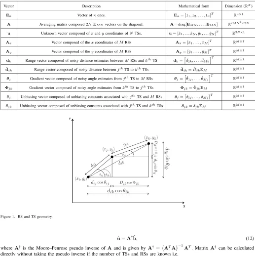
andDˆjksin ˆΦjk are subtracted, respectively, constituting the cooperation step. These operations can be understood from Fig.

1 in which the geometry of theith_{RS and that ofj}th _andkth_{TS is illustrated. To write (7) and (8) in matrix form we first}

define the vectors in table I:

Equ. (7) and (8) can then be represented in matrix form as

Aˆu=bˆ, (11)

ˆ

b= [bx₁, ...,bx_N,by₁, ...,by_N]T,

where

bx_j =



   

Ax+d1cosθ1δ1−dˇj1cosΦj1δj1

Ax+d2cosθ2δ2−dˇj2cosΦj2δj2 ..

.

Ax+dNcosθNδN −djNˇ cosΦjNδjN



   

, by_j =



   

Ay+d1sinθ1δ1−dˇj1sinΦj1δj1

Ay+d2sinθ2δ2−dˇj2sinΦj2δj2 ..

.

Ay+dNsinθNδN−djNˇ sinΦjNδjN



   

The LLS solution for the linear system is given by

Table I NOTATIONS.

Vector Description Mathematical form Dimension (RX₎

E_{κ Vector ofκones.} E_{κ= [11,12, . . . ,1κ]}T _Rκ×1

A _{Averaging matrix composed2N}E_{M N vectors on the diagonal.} A_{= diag[}E_{M N, . . . ,}E_{M N] R}2M N2×2N

u _{Unknown vector composed ofxandycoordinates ofNTSs.} u_{= [ˆx1, . . .xˆ}

N,ˆy1, . . .ˆyN]T R2N×1 A_{x Vector composed of thexcoordinates ofM RSs} A_{x= [¯x1, . . . ,x¯M]}T _RM×1

A_{y Vector composed of theycoordinates ofM RSs} A_{y= [¯y1, . . . ,y¯}

M]T RM×1

d_{k Range vector composed of noisy distance estimates betweenM RSs andk}th_TS d_k=h_dˆ_{1k, . . . ,d}ˆ_{M k}iT _RM×1

ˇ

d

jk Range vector composed of noisy distance betweenjthTS tokthTSs dˇjk= ˆDjkEM RM×1 θ_j Gradient vector composed of noisy angle estimates fromjth_{TS toMRSs θ}

j=

h

ˆ

θ1j, . . . ,θˆM j

iT

RM×1

Φ

jk Gradient vector composed of noisy angle estimates fromkthTS tojthTSs Φjk= ˆΦjkEM RM×1 δ_j Unbiasing vector composed of unbiasing constants associated withjth_{TS andM RSs δ}

j=

δ1j, . . . , δM j

T

RM×1

δ_{jk Unbiasing vector composed of unbiasing constants associated with}jth_{TS andk}th_{TSs δ}

[image:5.612.48.565.82.600.2]

jk=δjkEM RM×1

Figure 1. RS and TS geometry.

ˆ

u=A†bˆ, (12)

where A† _{is the Moore–Penrose pseudo inverse of A and is given by A}† _{= A}T_A−1

AT_{. MatrixA}† _{can be calculated}

directly without taking the pseudo inverse if the number of TSs and RSs are known i.e.

A† = diag [η,η,· · ·,η] ∈ R2N×2M N2, (13) whereη is a row matrix ofM N elements, the value of each element is given by _{M N}1 .This cooperative LLS estimator (12) shall be referred to as LLS-Coop in the rest of the paper.

A. Distributed Approach

If only one or a subset of all the TSs is desired to be localised while capitalizing on the cooperation with all TSs but avoiding the complexity of the centralized algorithm as in the previous case, a distributed approach can be employed. The distributed cooperative localisation, localises a single TS (this can be easily extended to estimate the location of a subset of all TSs) and reduces the complexity of the system without affecting the accuracy of localisation.

The location estimate of thejth

TS is given by

Ajˆuj =bjˆ ,

where

Aj = diag [E,E] ∈ R2M N×2,

uj = [xj, yj] T

∈ R2×1,

ˆ bj=

bx_j,by_jT

,

The LLS solution is then given by

ˆ

uj =A†jbˆj

for A†_j = diag [η,η] ∈ R2×2M N.

B. Cooperative Hybrid AoA-ToA

From here onwards, for cooperative hybrid AoA-ToA, dˆij, Dˆij and δij will be represented by dˆT ,ij, DˆT ,ij and δT ,ij

respectively, and are given by

ˆ

dT ,ij=dij+nij,

ˆ

DT ,jk=Djk+njk,

δT ,ij= exp

σm2ij

2

!

,

wheredij =

q

(¯xi−xj)

2

+ (¯yi−yj)

2

andDjk=

q

(xj−xk)

2

+ (yj−yk)

2

,nij andnjkrepresent the zero mean Gaussian

errors in distance estimates i.e. nij ∼ N

0, σ2nij

andnjk ∼ N

0, σ2njk

.The angle measurement θˆij from thejth TS to

ith

RS is given by

ˆ

θij = arctan

₍

yj−y¯i) (xj−¯xi)

+mij, (14)

wheremij represents the zero mean Gaussian error in angle estimates i.e.mij ∼ N

0, σ2

mij

.On the other hand, the angle measurement between from kth

tojth

TS i.e.Φjkˆ can be obtained in one of the following ways.

Case 1. If all TSs are capable of estimating their relative angles thenΦjkˆ can be modelled as

ˆ

Φjk= arctan

₍

yk−yj) (xk−xj)

+mjk, (15)

wheremjk represents the zero mean Gaussian noise in angle estimate i.e. mjk∼ N

0, σ2mjk

.

Case 2. In many cases, only the RSs are capable of AoA measurements while the TSs are low in resources and hence can

only estimate their relative distances, in other words the TSs are not hybrid, then for the formulation in (11), Φjkˆ can be estimated as follows

ˆ

Φjk= arctan

_(ˆ

yk−yˆj) (ˆxk−xˆj)

, (16)

where the (ˆyk−yˆj) and (ˆxk−xˆj) in (16) are estimated using (9) and (10) respectively. The performance of the system

decreases in this case as the number of observations decreases. These systems where the TSs are not hybrid will be referred to as LLS-Coop-X.

c_xt_{,k = d}2 ik 2 + σ2 nik 2

exp σ2mik

+

_d2

ik

2 cos (2θik) +

σ2

nik

2 cos (2θik)

exp −σm2ik

−(dikcosθik)2 (19)

cty,k =

d2ik 2 +

σn2ik

2

exp σ2mik

−

d2ik

2 cos (2θik) +

σ2nik

2 cos (2θik)

exp −σ2mik

−(diksinθik)2 (20)

c_xR_{,k =} d

2

ik 2 exp

σ2wik

(γα)2+σ

2 mik ! +d 2 ik

2 cos (2θik) exp

σ2wik

(γα)2−σ

2

mik

!

−(dikcosθik)

2

(21)

cRy,k=

d2ik 2 exp

σw2ik

(γα)2+σ

2 mik ! −d 2 ik

2 cos (2θik) exp

σ2wik

(γα)2−σ

2

mik

!

−(diksinθik)

2

(22)

C. Cooperative Hybrid AoA-RSS

For hybrid AoA-RSS, dˆij, Dˆjk and δij are represented by dˆR,ij, DˆR,ij andδR,ij respectively and are estimated from the

RSS measurements as in [23].

ˆ

dR,ij=dijexp

wij γα , ˆ

DR,jk=Djkexp

wjk

γα

,

δR,ij = exp

σ2mij

2 −

σ2wij

2 (γα)2

!

,

wherewij is the zero mean Gaussian random variable representing the shadowing effects i.e.wij∼ N

0, σ2

wij

.θˆij andΦjkˆ

are the same for both models given by (14), (15) and (16).

IV. LLS OPTIMISATION

In this section, we improve the performance of the LLS by proposing an optimisation step. In order to localise TS j with coordinates(xj, yj), the cooperation steps with TSkwith coordinates(xk, yk)are represented by (7) and (8), wheredˆikcos ˆθik

is the projection ofdˆik on thex−axis anddˆiksin ˆθikis the projection ony−axis. In the formulation (7) and (8), the projection

of Dˆjk i.e.Dˆjkcos ˆΦjk andDˆjksin ˆΦjk are subtracted from dˆikcos ˆθik anddˆiksin ˆθik respectively for all M RSs. Since the

combined error in hybrid distance and angle measurements is inherently distance dependent, step (7) and (8) may introduce large error if some RSs are positioned far away from the TS. Thus, instead of using all RSs, a pair of optimal RSs could be selected that guarantees minimum error or the RSs with the least error in the projectiondˆikcos ˆθikanddˆiksin ˆθikis selected. In

this section, we propose an optimisation scheme that will select such a pair of RSs. Let the total number of RSs be represented by the setRS ={RS1,RS2,· · · ,RSM}, then the number of 2-subsetsRSsub⊂RSis given by the permutation with repetition i.e. M2. Then to localise thejth_{TS in cooperation with thek}th_{TS, the first optimal RSRS}

opt(1)ofRSsubis selected as the one that minimises the approximate variance of the projectiondˆikcos ˆθik such that

RSopt(1)= arg min RS∈RS

{c_{x,k}. (17)}

and the second RS RSopt(2) is selected as the one that minimises the projectiondˆiksin ˆθiksuch that RSopt(2)= arg min

RS∈RS

{c_{y,k}. (18)}

c_{x,k and cy,k represent the approximate variance of the respective projections of d}ˆ_{ik. They are represented by} ct x,k and ct

y,k and are given by (19) and (20) for AoA-ToA respectively [20]. On the other hand, they are represented by c

R x,k andc

R y,k

and given by (21) and (22) for AoA-RSS respectively [19]. Since the actual value of the distance in (19)-(22) is unknown its estimated value is used. It should be noted that the same RS could serve as the optimal RS to minimise both (17) and (18). The LLS estimator with this optimisation shall be referred to as LLS-Opt-Coop.

Table II

COMPUTATION COMPLEXITY.

Operation MUL ADD CMP CPU cycles(M= 3, N= 5)

AoA-ToA AoA-RSS AoA-ToA AoA-RSS AoA-ToA AoA-RSS

LLS-NoCoop

NA

A† _{1 1 0 0 3 3}

b _{22M N 26M N 10M N 12M N 1140 1350}

A†b _{4M N 4M N (4M N}−2N) (4M N−2N) 230 230

LLS-Coop

NA

A† _{2 2 0 0 6 6}

b _22N(M+N−1) 26N(M+N−1) 10N(M+N−1) 12N(M+N−1) 2660 3150

A†b _{4M N}3 _{4M N}3 _{4M N}3_−2N

4M N3_−2N

5990 5990

LLS-Opt-Coop

2M N

A† _{1 1 2 2 5 5}

b _22N(M+N−1) 26N(M+N−1) 10N(M+N−1) 12N(M+N−1) 2660 3150

A†b _4N2₍M+N−1) 4N2

(M+N−1) 4N2

(M+N−1)−2N 4N2

(M+N−1)−2N 2790 2790

App. Var 74M N 62M N 36M N 24M N 3870 3150

Cycle count for CMP - - - - 30 30

TSA

TSE

TSD

TSC

TSB

30 m eters

Figure 2. Network topology for localisation of TSAwith a communication range of 30m.

V. PARTIALCONNECTIVITY

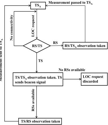
Full connectivity can not always be achieved in large networks due to limited communication range of resource constraint sensor nodes. Hence the assumption of full connectivity becomes unrealistic in large networks. In this section, we explore the issue of partial connectivity in cooperative hybrid networks. A TSA(TS that is to be localised) first broadcasts a location request message (LOC request), which is picked up by other TSs, RSs or in most cases both. In the second step is, if an RS receives the LOC request it measures the range and the angle of the impinging signal and send the measurements back to TSA. On the other hand, if another TS receives the LOC request it has to check for the availability of RSs in its own range. If no RSs are available, the LOC request is discarded by the TS. In case of availability of one or more RSs, the measurements (RS-TSA and TS-TSA observations) are passed to TSA. If the LOC request is not picked by any sensor node, then TSAis out of communication range of the network and cannot be localised. The network topology for the localisation of TSA with a communication range of 30 meters is shown in Fig. 2. It should be noted that with this communication range, TSA can not establish a communication link directly with any RS. The scenario presented in Fig. 2 is taken from the network deployment used in the simulation section given in Fig. 4. In Fig. 2 three types of communication links are shown, dashed, bold and zigzag. Zigzag lines represents a direct communication link with the RSs. Bold lines represents a links between two TSs that are utilized in a cooperative manner for localisation as explained in section III. It should be noted that TSAis directly connected TSC,however the link between them is represented by a dashed line showing that the angle and range measurement between TSA and TSCcannot be utilized for localisation of TSA.This is because TSC is not in range of any RSs. These steps can be understood from Fig. 3. A pseudocode for the localisation of TSA is given in Algorithm 1.

VI. COMPLEXITYANALYSIS

In this section, we present the complexity analysis of the proposed algorithms. Following [24], the CPU cycle count is used to compare the computational complexities by considering the individual cycle counts for addition (ADD), multiplication

Algorithm 1 Pseudocode for localisation of TSA. PROGRAM : Partial connectivity

1) TSA broadcasts LOC 2) Pause(time)

3) IFTSA receive measurements from RSs or TSs. 4) identify transmitter

5) IFtransmitters are only RSs 6) Localise via (9) and (10) only. 7) ELSE IFtransmitters are TSs 8) Localise via (7) and (8) only.

9) ELSE IFtransmitters are RSs and TSs. 10) Localise via (7), (8), (9) and (10). 11) ENDIF

12) ELSE

13) TSA is outside the networks range. 14) END

TS_A

RS/TS

LO

C

r

e

q

u

e

st

RS/TSAobservation taken

RS

Measurement passed to TSA

N

o

c

on

n

e

c

ti

vi

ty

TS/TSAobservation taken. TS

sends beacon signal TS

LOC request discarded No RSs available

TS/RS observation taken

R

S

s a

v

a

il

a

b

le

M

e

a

su

r

e

m

e

n

t

se

n

t

to

TS

[image:9.612.229.414.269.483.2]

A

Figure 3. Flowchart for localisation of TSAin case of full and partial connectivity.

(MUL), and comparison (CMP) operations. Thus using cycle count 1, 3 and 1 for ADD, MUL and CMP respectively, the complexities of LLS-NoCoop, LLS-Coop and LLS-Opt-Coop are given in table II. For LLS-NoCoop the complexity shown in table II is for all N TSs localised individually without cooperation. The CMP operator is only used in LLS-Opt-Coop to compare the approximate variances given by (19), (20) and (21), (22) for AoA-ToA and AoA-RSS signal models respectively. The number of comparison required for each model is 2M N. Number of cycles counts for calculating approximate variance is given by App. Var in table II. For complexity analysis given in table II, we consider 4 RSs and 5 TSs. Table II shows that the CPU cycle count for LLS-NoCoop is the lowest, followed by LLS-Coop and then LLS-Opt-Coop.

VII. SIMULATIONRESULTS

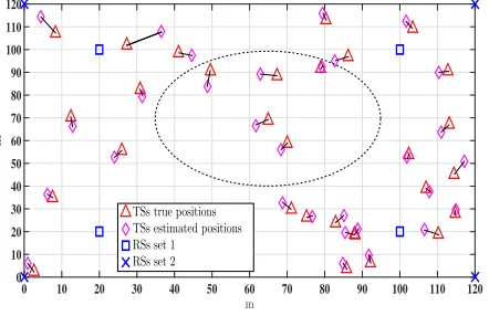
We consider a 120m×120m network with two sets of RSs; RSs set 1 and RSs set 2 with locations

(20,20),(20,100),(100,20)(100,100) and (0,0),(0,120),(120,0)(120,120), respectively. Also 30 TSs are deployed at random locations. All the simulations are run independently υ number of times. For simplicity, the same noise variance in distance and angle measurements is used for all RS-TS and TS-TS links i.e. σ2nij =σ

2

njk =σ

2

n andσm2ij =σ

2

mjk =σ

2

m. The

network deployment is shown in Fig. 4.

In Fig. 5 the proposed LLS-Coop, LLS-Coop-X and LLS-Opt-Coop are compared with the iterative NLLS algorithm presented by (1). The MatLab function fminsearch, which is based on Nelder-Mead simplex algorithm [25], is used for the minimisation of (1). For this simulation, it was noted that the cost function failed to converge when RSs set 1 was

m

0 10 20 30 40 50 60 70 80 90 100 110 120

m 0 10 20 30 40 50 60 70 80 90 100 110 120

[image:10.612.209.430.58.201.2]

TSs true positions TSs estimated positions RSs set 1 RSs set 2

Figure 4. Network deployment with true and estimated locations with LLS-Coop using AoA-RSS signal model. RSs set 1,σ2

wij =σ

2

wjk =σ

2 w= 4 dB,

σ2mij=σ 2

mjk=σ

2

m= 4

o

,υ= 1500, αi∀i= 2.5.

σ2n(m

2₎

1 1.5 2 2.5 3 3.5 4 4.5 5 5.5 6 2 3 4 5 6 7 8 9 10 11 12 13

Iterative hybrid AoA-ToA LLS-Coop-X LLS-Coop LLS-Opt-Coop

σ2

m(deg)

1 1.5 2 2.5 3 3.5 4

Av g. R M S E ( m ) 2 3 4 5 6 7 8 9 10 11 12 13

(a) Performance comparison for AoA-ToA signal model. RSs set 2,υ= 1000.

σ2w(dB)

1 1.5 2 2.5 3 3.5 4 4.5 5 5.5 6 2 4 6 8 10 12 14 16 18

Iterative hybrid AoA-RSS LLS-Coop-X LLS-Coop LLS-Opt-Coop

σm(deg)2

1 1.5 2 2.5 3 3.5 4 4.5 5 5.5 6

Av g. R M S E ( m ) 2 4 6 8 10 12 14 16 18

[image:10.612.99.524.279.421.2]

(b) Performance comparison for AoA-RSS signal model. RSs set 2,υ= 1000, αi∀i= 2.5.

Figure 5. Performance comparison of the proposed algorithms with NLLS iterative hybrid algorithm.

used. This is because a number of TSs lies in a region outside the convex hull defined by the RSs set 1. In order to guarantee convergence RSs set 2 was used for this simulation. As evident from Fig. 5a and Fig. 5b that our proposed cooperative algorithms are more reliable than the NLLS iterative hybrid algorithm [15].

In Fig. 6, the hybrid AoA-ToA algorithms are compared in terms of Avg. RMSE while the variance in distance and angle estimates is increased. It is seen that the performance of the LLS estimator with no cooperation (LLS-NoCoop) is worst of all. Considerable performance improvement is observed with cooperation between the TSs; with the LLS-Opt-Coop estimator showing the lowest RMSE. Next is the LLS-Coop when both TSs and RSs are hybrid. While performance degradation is observed for LLS-Coop-X i.e. when the TSs are not hybrid.

Fig. 7 presents the performance of AoA-RSS hybrid systems, the RMSE in location estimates is compared when the shadowing variance and the angle error variance is incremented in the links. Shadowing variance is kept the same for all links i.e. σ2

wij =σ

2

wjk =σ

2

w. Altogether the performance is worst than the AoA-ToA case, this is due to the fact that the RSS

distance estimates are more erroneous then the ToA distance estimates, especially at longer inter-node distance. The PLE value considered is 2.5, and is the same for all links. A similar trend as in Fig. 6 is observed in this case, with LLS-Opt-Coop performing the best followed by LLS-Coop and then LLS-Coop-X while the LLS-NoCoop performs the worst.

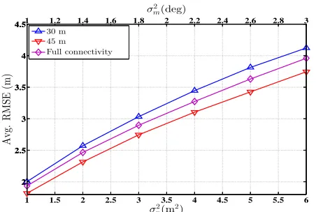
Fig. 8 shows the performance of LLS-Coop AoA-ToA model when the network is not fully connected. It is noted that the full connectivity does not give the best performance. This is because the angle noise variance is distance dependent, hence in case of full connectivity the noisy links with far away sensor nodes are also utilized which degrades the overall performance of the system.

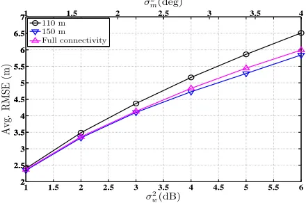
A similar trend is seen in Fig. 9 where the performance of LLS-Coop for AoA-RSS model is compared for different connectivity ranges. In this case both angle and range noise variance are distance dependent. A full connectivity does not show the best performance in this case either.

1 1.5 2 2.5 3 3.5 4 4.5 5 5.5 6 2

3 4 5 6 7 8 9 10 11 12 13

σ2n(m 2₎

0 0.5 1 1.5 2 2.5 3 3.5 4

2 3 4 5 6 7 8 9 10 11 12 13

σ2m(deg)

Av

g.

R

M

SE

(m

)

[image:11.612.193.416.86.231.2]

LLS-NoCoop LLS-Coop-X LLS-Coop LLS-Opt-Coop

Figure 6. Performance comparison between LLS-NoCoop, LLS-Coop, LLS-Coop-X, LLS-Opt-Coop hybrid AoA-ToA localisation. RSs set 1,υ= 1500.

1 1.5 2 2.5 3 3.5 4 4.5 5 5.5 6

2 4 6 8 10 12 14 16 18

σw2(dB)

1 1.5 2 2.5 3 3.5 4

2 4 6 8 10 12 14 16 18

σm2(deg)

Av

g.

R

M

SE

(m

)

LLS-NoCoop LLS-Coop-X LLS-Coop LLS-Opt-Coop

Figure 7. Performance comparison between LLS-NoCoop, LLS-Coop, LLS-Coop-X, LLS-Opt-Coop hybrid AoA-RSS localisation. RSs set 1,υ= 1500, αi∀i= 2.5.

1 1.5 2 2.5 3 3.5 4 4.5 5 5.5 6

2 2.5 3 3.5 4 4.5

σn2(m

2₎

1 1.2 1.4 1.6 1.8 2 2.2 2.4 2.6 2.8 3

2 2.5 3 3.5 4 4.5

σ2m(deg)

Av

g.

R

M

SE

(m

)

30 m 45 m Full connectivity

Figure 8. Performance comparison for LLS-Coop AoA-ToA model with partial connectivity,σ2

nij = σ

2

njk = σ

2

n ,σ

2

mij =σ

2

mjk = σ

2

m, RSs set 1,

υ= 1500.

[image:11.612.195.413.315.464.2] [image:11.612.189.415.549.701.2]

1 1.5 2 2.5 3 3.5 4 4.5 5 5.5 6 2

2.5 3 3.5 4 4.5 5 5.5 6 6.5 7

σw2(dB)

1 1.5 2 2.5 3 3.5 4

2 2.5 3 3.5 4 4.5 5 5.5 6 6.5 7

σm2(deg)

Av

g.

R

M

SE

(m

)

110 m 150 m Full connectivity

Figure 9. Performance comparison for LLS-Coop AoA-RSS model with partial connectivity. RSs set 1, σ2

wij =σ

2

wjk =σ

2

w ,σ

2

mij =σ

2

mjk =σ

2 m,

υ= 1500, αi∀i= 2.5.

VIII. CONCLUSION

In this paper two hybrid localisation models were analysed. These hybrid signal models were extended to their respective cooperative forms and TS-TS links were utilized. Hence a LLS cooperative location scheme for the hybrid AoA-ToA and AoA-RSS signals were proposed. A distributed version was also presented to estimate the location of a subset of the total number of TSs. A modified approach was proposed when the TSs are not hybrid and can only estimate distance from other sensors. Moreover an optimisation technique based on the selection of a pair of optimal RSs was proposed. Furthermore both models were studied for partial connectivity between sensor nodes. Finally complexity of the algorithms was analysed and it was proved via simulation that the cooperative technique performs considerably better than its non-cooperative counterpart, while its performance is further improved using the optimisation technique.

REFERENCES

[1] J. Ko, T. Gao, R. Rothman, and A. Terzis, “Wireless sensing systems in clinical environments: Improving the efficiency of the patient monitoring process,”IEEE Engineering in Medicine and Biology Magazine, vol. 29, no. 2, pp. 103–109, March 2010.

[2] P. Juang, H. Oki, Y. Wang, M. Martonosi, L. S. Peh, and D. Rubenstein, “Energy-efficient computing for wildlife tracking: Design tradeoffs and early experiences with zebranet,”SIGARCH Comput. Archit. News, vol. 30, no. 5, pp. 96–107, Oct. 2002.

[3] I. Guvenc and C.-C. Chong, “A survey on TOA based wireless localization and NLOS mitigation techniques,”IEEE Communications Surveys Tutorials, vol. 11, no. 3, pp. 107–124, 2009.

[4] N. Salman, M. Ghogho, and A. H. Kemp, “On the joint estimation of the RSS-based location and path-loss exponent,”IEEE Wireless Communications Letters, vol. 1, no. 1, pp. 34–37, 2012.

[5] P. Kulakowski, J. Vales-Alonso, E. Egea-López, W. Ludwin, and J. García-Haro, “Angle-of-arrival localization based on antenna arrays for wireless sensor networks,”Computers & Electrical Engineering, vol. 36, no. 6, pp. 1181 – 1186, 2010.

[6] H.-C. Chen, T.-H. Lin, H. Kung, C.-K. Lin, and Y. Gwon, “Determining RF angle of arrival using COTS antenna arrays: A field evaluation,” inMilitary Communications Conference, pp. 1–6, 2012.

[7] A. Nasipuri and K. Li, “A directionality based location discovery scheme for wireless sensor networks,” inProceedings of the 1st ACM International Workshop on Wireless Sensor Networks and Applications. ACM, pp. 105–111, 2002.

[8] N. Patwari, J. Ash, S. Kyperountas, A. Hero, R. Moses, and N. Correal, “Locating the nodes: cooperative localization in wireless sensor networks,”

IEEE Signal Processing Magazine, vol. 22, no. 4, pp. 54–69, 2005.

[9] J. A. Costa, N. Patwari, and A. O. Hero, III, “Distributed weighted-multidimensional scaling for node localization in sensor networks,”ACM Trans. Sen. Netw., vol. 2, no. 1, pp. 39–64, Feb. 2006.

[10] W. S. Torgerson, “Multidimensional scaling: I. theory and method,”Psychometrika, vol. 17, pp. 401–419, 1952.

[11] B. Xia, L. Zhang, Q. Liu, and Z. Liu, “An improved mds algorithm for wireless sensor network,” inBiomedical Engineering and Computer Science (ICBECS), 2010 International Conference on, April 2010, pp. 1–4.

[12] W. Shi and V. Wong, “MDS-based localization algorithm for RFID systems,” inIEEE International Conference on Communications (ICC), 2011, pp. 1–6.

[13] C.-H. Wu, W. Sheng, and Y. Zhang, “Mobile sensor networks self localization based on multi-dimensional scaling,” inRobotics and Automation, 2007 IEEE International Conference on, 2007, pp. 4038–4043.

[14] I. Borg and P. Groenen,Modern Multidimensional Scaling: Theory and Applications. Springer, 2005.

[15] G. Ding, Z. Tan, L. Zhang, Z. Zhang, and J. Zhang, “Hybrid TOA/AoA cooperative localization in non-line-of-sight environments,” in IEEE 75th Vehicular Technology Conference (VTC Spring), May 2012, pp. 1–5.

[16] L. Gazzah, L. Najjar, and H. Besbes, “Hybrid RSSD/AoA cooperative localization for 4g wireless networks with uncooperative emitters,” inIn Proc. International Wireless Communications and Mobile Computing Conference (IWCMC), Aug 2015, pp. 874–879.

[17] S. Frattasi and M. Monti, “On the use of cooperation to enhance the location estimation accuracy,” in 3rd International Symposium on Wireless Communication Systems, 2006, Sept 2006, pp. 545–549.

[18] M. Khan, N. Salman, and A. H. Kemp, “Cooperative positioning using angle of arrival and time of arrival,” inSensor Signal Processing for Defence (SSPD), pp. 1–5, Sept 2014.

[19] N. Salman, M. W. Khan, and A. H. Kemp, “Enhanced hybrid positioning in wireless networks II: AoA-RSS,” inIEEE International Conference on Telecommunications and Multimedia (TEMU), pp. 92–97, July 2014.

[20] M. Khan, N. Salman, and A. H. Kemp, “Enhanced hybrid positioning in wireless networks I: AoA-ToA,” in IEEE International Conference on Telecommunications and Multimedia (TEMU), pp. 86–91, July 2014.

[image:12.612.193.413.63.209.2]

[21] N. Salman, A. H. Kemp, and M. Ghogho, “Low complexity joint estimation of location and path-loss exponent,”IEEE Wireless Communications Letters,, vol. 1, no. 4, pp. 364–367, 2012.

[22] X. Li, “RSS-based location estimation with unknown pathloss model,”IEEE Transactions on Wireless Communications,, vol. 5, no. 12, pp. 3626–3633, 2006.

[23] N. Salman, M. Ghogho, and A. Kemp, “Optimized low complexity sensor node positioning in wireless sensor networks,”Sensors Journal, IEEE, vol. 14, no. 1, pp. 39–46, 2014.

[24] I. Guvenc, S. Gezici, and Z. Sahinoglu, “Fundamental limits and improved algorithms for linear least-squares wireless position estimation.”Wireless Communications and Mobile Computing, vol. 12, no. 12, pp. 1037–1052, 2012.

[25] J. C. Lagarias, J. A. Reeds, M. H. Wright, and P. E. Wright, “Convergence properties of the nelder-mead simplex method in low dimensions,”SIAM Journal of Optimization, vol. 9, pp. 112–147, 1998.