This is a repository copy of
Non parametric directionality analysis - extension for removal
of a single common predictor and application to time series
.
White Rose Research Online URL for this paper:
http://eprints.whiterose.ac.uk/99679/
Version: Accepted Version
Article:
Halliday, David M orcid.org/0000-0001-9957-0983, Senik, Mohd Harizal, Stevenson, Carl
W et al. (1 more author) (2016) Non parametric directionality analysis - extension for
removal of a single common predictor and application to time series. Journal of
Neuroscience Methods. pp. 87-97. ISSN 0165-0270
https://doi.org/10.1016/j.jneumeth.2016.05.008
[email protected] https://eprints.whiterose.ac.uk/
Reuse
Items deposited in White Rose Research Online are protected by copyright, with all rights reserved unless indicated otherwise. They may be downloaded and/or printed for private study, or other acts as permitted by national copyright laws. The publisher or other rights holders may allow further reproduction and re-use of the full text version. This is indicated by the licence information on the White Rose Research Online record for the item.
Takedown
If you consider content in White Rose Research Online to be in breach of UK law, please notify us by
Non parametric directionality analysis - extension for removal of a single common
predictor and application to time series.
David M. Hallidaya,∗, Mohd Harizal Senikb, Carl Stevensonc, Rob Masonb
a
Department of Electronics, University of York, YORK YO10 5DD, UK
bSchool of Life Sciences, University of Nottingham, Nottingham, NG7 2UH, UK c
School of Biosciences, University of Nottingham, Loughborough LE12 5RD, UK
Abstract
Background. The ability to infer network structure from multivariate neuronal signals is central to computational neuroscience. Directed network analyses typically use parametric approaches based on auto-regressive (AR) models, where networks are constructed from estimates of AR model parameters. However, the validity of using low order AR models for neurophysiological signals has been questioned. A recent article introduced a non parametric approach to estimate directionality in bivariate data, non parametric approaches are free from concerns over model validity.
New Method. We extend the non parametric framework to include measures of directed conditional independence, using scalar measures that decompose the overall partial correlation coefficient summatively by direction, and a set of functions that decompose the partial coherence summatively by direction. A time domain partial correlation function allows both time and frequency views of the data to be constructed. The conditional independence estimates are conditioned on a single predictor.
Results. The framework is applied to simulated cortical neuron networks and mixtures of Gaussian time series data with known interactions. It is applied to experimental data consisting of local field potential recordings from bilateral hippocampus in anaesthetised rats.
Comparison with Existing Method(s). The framework offers a non parametric approach to estimation of directed interactions in multivariate neuronal recordings, and increased flexibility in dealing with both spike train and time series data.
Conclusions. The framework offers a novel alternative non parametric approach to estimate directed interactions in multivariate neuronal recordings, and is applicable to spike train and time series data
Keywords: Directionality, Partial Coherence, Non parametric, Time series, Point process, Conditional independence, Granger causality
1. Introduction
Directed network analyses are widely used in neuro-science to infer network structure in multivariate neural recordings (Rubinov and Sporns, 2010). The majority of approaches are parametric, which rely on estimating the parameters of a model to describe the patten of interac-tions between the observed signals, typically using auto-regressive (AR) models (Granger, 1969; Geweke, 1982). Once the AR parameters have been estimated different metrics relating to directionality can be constructed di-rectly as a function of the model parameters (Baccala et al., 2001; Kaminski et al., 2001; Chen et al., 2006; Schel-ter et al., 2006; Chicharro, 2012). A number of concerns have been raised regarding the validity of AR models to accurately capture the complex structure present in multi-variate neural and other time series typically encountered
∗Corresponding author
Email address: [email protected](David M. Halliday)
in scientific problems (Gersch, 1972; Thomson and Chave, 1991; Lindsay and Rosenberg, 2011). A number of alter-native non parametric approaches have been considered to describe directed interactions in neurophysiological signals (Gersch, 1972; Eichler et al., 2003; Lindsay and Rosenberg, 2011). A recent article introduced a non parametric frame-work for directionality analysis of bivariate data (Halliday, 2015), with application to single unit spike train data.
can be derived. An alternative parametric approach using information theoretic measures (Geweke, 1982) has also been extended to include conditioning variables (Pierce, 1982; Geweke, 1984). Related approaches are considered in Chen et al. (2006); Guo et al. (2008).
This paper presents a novel extension to the non para-metric approach in Halliday (2015) for multivariate data by presenting a framework for analysis of three random processes. We also investigate applicability of the frame-work to both time series data and spike train data. One advantage of considering time series data is that measures derived from residual and conditional variance metrics can readily be calibrated against known (simulated) data. We undertake such a comparison to establish the accuracy and usefulness of our multivariate extension. The approach is further validated through application to experimental data consisting of local field potential recordings from bilateral hippocampus in anaesthetised rat. Our results demon-strate the flexibility of the non parametric approach in dealing with both spike train and time series data. Our novel approach should therefore have broad applicability across a wide range of electrophysiological data.
The paper is arranged as follows. Section 2 presents the methods including sub-sections on algorithms and signifi-cance testing. Section 3 describes results from application of the conditional non parametric framework to simulated cortical neuron networks, to artificial mixtures of Gaus-sian time-series used to verify quantitative aspects of the framework and to the experimental data. Conclusions and discussion are in section 4.
2. Methods
Our framework assumes that random processes have wide-sense (weak) stationarity (Brillinger, 1975; Priestley, 1981). The approach can be applied to time series data and point-process data. Point process data are represented using differential increments which count the number of spikes in a small interval, which we assume to be the sam-pling interval ∆t(Rosenberg et al., 1989; Conway Halliday and Rosenberg, 1993). Point processes are also assumed to be orderly, i.e. only one spike can occur in each sampling interval (Conway Halliday and Rosenberg, 1993). In the derivation below (x, y, z) refer to three random processes which can be either time series or point process differential increments, or mixtures of the two data types. We use the term multivariate in the manuscript, since we are consid-ering the analysis of three simultaneous random processes. However, only a single predictor is used, the possibility of extending the analysis to multiple predictors is considered in the discussion.
2.1. Theory
For bivariate random processes (x, y) a scalar measure of overall dependence is given by the squared correlation
coefficient (Pierce, 1979; Halliday, 2015). This is defined in terms of ordinary and residual variances as
R2yx= (σ2y−σ2y|x)/σy2 (1)
The conditioned variance,σ2
y|xcan be equated to the
vari-ance of the error process after a linear regression ofy on
x. Equation 1 can be interpreted as the fraction of the variance inythat can be accounted for by the regressorx. It is a symmetrical measure which does not provide any indication of directionality of interaction.
To account for any common effect that processz may have on bothxand y a partial correlation coefficient can be used
R2yx|z= (σ2y|z−σ2y|x,z)/σ2y|z (2)
In this case both processes x and y are conditioned on the third process z. Partial regression is widely used in situations where it is believed that the predictor, z, can account for some or all of the original association between
xandy. The objective is to distinguish a genuine correla-tion,R2
yx|z, from an apparent or induced correlation,Ryx2 .
Throughout this paper we use linear models and consider linear interactions.
The relationship between the scalarR2
yxand the
coher-ence function,|Ryx(λ)|2was used as the starting point for
the derivation of non parametric directionality measures in Halliday (2015). The frequency domain equivalent of the partial regression coefficient, equation 2, is the partial coherence function
|Ryx|z(λ)|2= |
fyx|z(λ)|2
fxx|z(λ)fyy|z(λ)
(3)
where fyx|z(λ) is the partial cross power spectral density
(or partial cross-spectrum) between processesxandywith predictorz. The two partial auto-spectra arefxx|z(λ) and
fyy|z(λ). Partial coherence estimates have proved useful
in identifying direct interactions from common inputs in functional connectivity studies of neural circuits (Rosen-berg et al., 1998; Eichler et al., 2003; Salvador et al., 2005; Medkour et al., 2009).
The link between the partial coherence function in equa-tion (3) and the partial correlaequa-tion coefficient in equaequa-tion (2) can be made by considering the residual variance in the partial regression model,σ2
y|x,z. In the frequency domain
this residual variance is the residual spectrum fyy|x,z(λ).
Using the same derivation as the bivariate framework (Hal-liday, 2015) we can derive the result
Ryx|z(λ) 2
= fyy|z(λ)−fyy|x,z(λ)
fyy|z(λ)
(4)
We have used the partial gain function (Halliday et al., 1995), fyx|z(λ)
fxx|z(λ), in this derivation. Thus, as in the
function decomposes theR2value by frequency, thusR2 yx|z
can be recovered by integrating the partial coherence
Ryx2 |z=
1 2π
Z +π
−π
Ryx|z(λ) 2
dλ (5)
where the partial coherence is defined over the normalised angluar frequency range [−π,+π].
Application of the minimum mean square error (MMSE) pre-whitening step (Eldar and Oppenheim, 2003) is next applied to reduce the partial coherence to the partial cross spectrum. Directionality measures can be derived using a similar sequence of steps as in the bivariate case (Halli-day, 2015). The aim of the pre-whitening step is to reduce the two partial auto spectra to have the value 1 at each frequency in equation (3), which requires the application of two pre-whitening filters that must reflect the proper-ties of the two processesxandy and their relationship to the predictor,z. This can be achieved using pre-whitened conditional discrete Fourier transforms as described below. Auto spectra are traditionally defined in terms of the expectation operator as (Brillinger, 1975)
fxx(λ) = lim T→∞
1 2πTE
n
dT
x(λ)dTx(λ) o
(6)
fyy(λ) = lim T→∞
1 2πTE
n
dTy(λ)dTy(λ) o
(7) where dT
x(λ) and dTy(λ) are the finite Fourier transforms
of length T from processes xand y respectively, and the overbar indicates a complex conjugate. A finite Fourier transform conditioned on a third process,z, can be defined (Tick, 1963; Brillinger, 1988) as
dT
x|z(λ) =dTx(λ)−
fxz(λ)
fzz(λ)
dT
z(λ) (8)
dTy|z(λ) =dTy(λ)−
fyz(λ)
fzz(λ)d T
z(λ) (9)
The quantitiesfxz(λ),fyz(λ) andfzz(λ) are the two cross
spectra between the conditioning process,z and the origi-nal processes and the auto spectra ofz, respectively. Defin-ing conditioned Fourier transforms in this manner allows the partial auto spectra to be defined as
fxx|z(λ) = lim T→∞
1 2πTE
n
dTx|z(λ)dTx|z(λ) o
(10)
fyy|z(λ) = lim T→∞
1 2πTE
n
dTy|z(λ)dTy|z(λ) o
(11) The pre-whitening step is applied using an approach simi-lar to the bivariate case presented in Halliday (2015). Ex-tending the concept of the MMSE pre-whitening filter in-troduced in Eldar and Oppenheim (2003), we define the MMSE pre-whitening filters for the two partial spectra as
wxx|z(λ) =fxx|z(λ)−1/2 (12)
wyy|z(λ) =fyy|z(λ)−1/2 (13)
Using these filters the pre-whitened transforms can be gen-erated as
dwTx|z(λ) =dTx|z(λ)wxx|z(λ) (14)
dwT
y|z(λ) =dTy|z(λ)wyy|z(λ) (15)
Equations (14) and (15) mimic the frequency domain im-plementation applying pre-whitening filters to the pro-cessesxandythat was used in the bivariate case. The dif-ference here is that the output of the filters are conditioned Fourier transforms which are optimally pre-whitened. Auto spectra estimated by replacing the expectation in equa-tions (10) and (11) with ensemble or segment averaging will have the value 1 at all frequencies:
fxxw|z(λ) = 1, fyyw|z(λ) = 1 (16)
Estimation of the partial cross spectrum from the pre-whitened conditioned Fourier transforms, equations (14) and (15), will be equivalent to the partial coherence
R
w yx|z(λ)
2 = f w yx|z(λ)
2
(17) Conditioned directionality measures can then be de-rived from the pre-whitened partial cross spectrum,fw
yx|z(λ),
in a manner similar to the bivariate case (Halliday, 2015). The overall scalar measure of dependence betweenxand
y conditioned (linearly) onz,R2 yx|z, is
R2 yx|z=
1 2π
Z +π
−π f
w yx|z(λ)
2
dλ (18)
To decompose R2
yx|z by direction we define a correlation
function, ρyx|z(τ) which is the inverse Fourier transform
of the pre-whitened partial cross spectrum
ρyx|z(τ) =
1 2π
Z +π
−π
fw
yx|z(λ)eiλτdλ (19)
The function defined in equation (19) could be referred to as a lagged conditional correlation function betweenx
and y. Following Brillinger (1975), second order spectra are assumed periodic inλwith period 2π(Brillinger, 1975, Th 2.5.1). Decomposition ofR2
yx|z by lag is achieved as
R2yx|z= Z +∞
−∞ |
ρyx|z(τ)|2dτ (20)
The proof of this central result follows closely that for the bivariate case (Halliday, 2015), using Parseval’s theorem (Priestley, 1981). Adopting the same approach as in the bivariate case allows the overall dependence to be decom-posed summatively by direction
R2yx|z= Z
τ <0|
ρyx|z(τ)|2dτ+|ρyx|z(0)|2+ Z
τ >0|
ρyx|z(τ)|2dτ
which we write, with an obvious extension to the notation, as
R2yx|z=Ryx2 |z;−+Ryx2 |z;0+R2yx|z;+ (22)
In the frequency domain the decomposition also follows closely the approach adopted in the bivariate case. Thef′
measures are defined as
fyx′ |z;−(λ) =
Z
τ <0
ρyx|z(τ)e−iλτdτ (23)
fyx′ |z;0(λ) =ρyx|z(0) (24)
f′
yx|z;+(λ) = Z
τ >0
ρyx|z(τ)e−iλτdτ (25)
with decomposition of the partial coherence, |Ryx|z(λ)|2,
summatively at each frequency given by
|Ryx|z(λ)|2=|R′yx|z;−(λ)|2+|R′yx|z;0(λ)|2+|R′yx|z;+(λ)|2
(26) where theR′functions are scaled according to the relative magnitude of thef′ functions at each frequency as
|R′yx|z;−(λ)|2=
|f′
yx|z;−(λ)|2
|f′
yx|z;−(λ)|2+|f ′
yx|z;0(λ)|2+|f
′
yx|z;+(λ)|2
|Ryx|z(λ)|2
(27)
|R′yx|z;0(λ)|2=
|f′
yx|z;0(λ)|2 |f′
y|zx;−(λ)|2+|fy′|zx;0(λ)|2+|fyx′ |z;+(λ)|2
|Ryx|z(λ)|2
(28)
|R′yx|z;+(λ)|2 = |f′
yx|z;+(λ)|2 |f′
yx|z;−(λ)|2+|f ′
yx|z;0(λ)|2+|f
′
yx|z;+(λ)|2
|Ryx|z(λ)|2
(29) The validity of this decomposition in the bivariate case is discussed in Halliday (2015).
2.2. Algorithms
The directionality measures can be constructed as a straightforward extension to a typical multivariate spec-tral analysis. The conditional directionality measures, in this case, assume that three random processes,x,yandz, are available for analysis. The directionality measures are constructed using a two stage process. In the first stage the discrete Fourier transforms are calculated in the usual way, and estimates of second order spectra are calculated -these are the estimated auto spectra, ˆfxx(λj), ˆfyy(λj) and
ˆ
fzz(λj), along with the estimated cross spectra, ˆfyx(λj),
ˆ
fxz(λj) and ˆfyz(λj). Estimates are indicated through the
use of the hat symbol, ˆ, the λj are the Fourier
frequen-cies, and the terminology for cross spectra, ˆfyx(λj), treats
x as the reference (or input) process. A number of well documented approaches exist for construction of second
order spectral estimates. Here we use the average peri-odogram approach, described in detail in Halliday et al. (1995), which involves sectioning a record intoL sections each containingT data points, thus analysing a record of duration R = LT samples. Alternatively, the direction-ality measures could be derived from alternative spectral estimation procedures, for example using multi-taper esti-mates (Percival and Walden, 1993).
The second stage constructs the conditional direction-ality estimates starting from the discrete Fourier transform for each segment,l (l = 1, . . . , L), from processesxand y
which are referred to asdT
x(λj, l) anddTy(λj, l). The
condi-tioned Fourier transforms for each segment are constructed as
dTx|z(λj, l) =dTx(λj, l)−
ˆ
fxz(λj)
ˆ
fzz(λj)
dTz(λj, l) (l= 1, . . . , L)
(30)
dT
y|z(λj, l) =dTy(λj, l)−
ˆ
fyz(λj)
ˆ
fzz(λj)
dT
z(λj, l) (l= 1, . . . , L)
(31) This gives a conditioned Fourier transform for each seg-ment, l, that is conditioned on the (common) process z. The conditioning factors (or gains) fˆxz(λj)
ˆ
fzz(λj) and ˆ fyz(λj)
ˆ
fzz(λj) are
the same for each segment and use the spectral estimates constructed in the first stage analysis. The first order par-tial spectra are then estimated from the conditioned dis-crete Fourier transforms. Here an average is taken across segments, for processxthis is
ˆ
fxx|z(λj) = 1
2πLT
L X
l=1 d
T x|z(λj, l)
2
(32)
The 1
2πT factor follows the convention in the bivariate case.
A similar expression is used to estimate ˆfyy|z(λj). The
pre-whitening filters are constructed as ˆ
wxx|z(λj) = ˆfxx|z(λj)−1/2 (33)
ˆ
wyy|z(λj) = ˆfyy|z(λj)−1/2 (34)
The hat indicates that these are estimates constructed from a single realisation of the three processes. A different realisation will result in a different pair of pre-whitening filters, this will achieve the objective of pre-whitening the conditioned auto-spectral estimates to 1 at each frequency. The pre-whitened discrete Fourier transforms for each seg-ment,l are
dwxT|z(λj, l) =dTx|z(λj, l) ˆwxx|z(λj) (l= 1, . . . L) (35)
dwTy|z(λj, l) =dTy|z(λj, l) ˆwyy|z(λj) (l= 1, . . . L) (36)
Whitened partial auto and cross spectra are estimated us-ing expressions similar to equation (32). To ensure that the whitened conditional auto spectral estimates, ˆfw
and ˆfw
yy|z(λ), have the value 1 at all frequencies, the same
averaging (or weighted averaging) should be applied to the same data segments when calculating the whitened spec-tra. The partial coherence can then be obtained directly from the whitened partial cross spectrum as
|Rˆw
yx|z(λj)|2=|fˆyxw|z(λj)|2 (37)
From this the partial correlation function,ρyx|z(τ), is
esti-mated using a standard inverse Fourier transform of length
T (Halliday et al., 1995).
The estimation of the directional metrics, the overall measureR2
yx|zand directional componentsRyx2 |z;−,R2yx|z;0
andR2
yx|z;+are estimated from ˆρyx|z(τk) using the same
al-gorithms as in the bivariate case, by substituting ˆρyx|z(τk)
for ˆρyx(τk) (Halliday, 2015). The same substitution
al-lows the estimated f′ functions, ˆf′
yx|z;−(λj), ˆfyx′ |z;0(λj)
and ˆf′
yx|z;+(λj), to be obtained from ˆρyx|z(τk) and from
these the estimated conditioned directional coherence func-tions, |Rˆ′
yx|z;−(λj)|
2, |Rˆ′
yx|z;0(λj)| 2 and
|Rˆ′
yx|z;+(λj)| 2 by
direct substitution of the appropriate estimates into equa-tions (27) - (29). Algorithmic level descripequa-tions of the conditional, three variable, analysis and the unconditional, two variable (Halliday, 2015) analysis are given in the Ap-pendix.
2.3. Significance testing
The approach here follows that adopted in the bivariate case (Halliday, 2015). The scalar measure of overall con-ditional correlation, R2
yx|z is estimated by integration of
partial coherence estimates. Confidence limits on partial coherence estimates are used as an indicator of a statisti-cally significant interaction. The setting of significance levels for partial coherence estimates constructed using average periodograms over L segments can be found in Brillinger (1975); Rosenberg et al. (1989); Halliday et al. (1995). In particular an upper 95% confidence limit based on a null hypothesis of no correlation after removal of com-mon linear effects from a single predictor can be estimated as (Rosenberg et al., 1989)
1−0.051/(L−2) (38)
This confidence limit can be used to assess the significance of ˆR2
yx|z. We assume that significant values of ˆRyx2 |z will
result when the corresponding partial coherence estimate has significant values (at frequencies of interest).
The variance of the bivariate correlation function,ρyx(τ),
was considered in Halliday (2015). The expression in-volved integration over the product of the prewhitened spectra, which have the value 1 at all frequencies. We use the same approach for the multivariate correlation func-tion, except that the integration is over the product of the two pre-whitened partial spectrafw
xx|z(λ) andfyyw|z(λ).
Since these are similarly equal to 1 at all frequencies we
obtain the same result var
ρyx|z(τ) = 1/R.
Approxi-mate upper and lower 95% confidence limits can be set as
0±1√.96
R (39)
whereR=LT, the total number of points analysed. The interpretation in the multivariate case is similar to that for the bivariate case. Significant values of ˆρyx|z(τ) at lags
τ <0 indicates a significantR2
yx|z;−, and significant values
of ˆρyx|z(τ) at lagsτ >0 indicates a significantR2yx|z;+. A
significant value of ˆρyx|z(0) indicates a significantR2yx|z;0.
The validity of equation (39) was checked using Monte-Carlo simulations using three examples of time series data (rows 1, 3, 5 from Table 1) and three examples of spike train data (configurations a and b from Figure 1 and 1 set of Poisson spike trains). In each example 100 repeat runs were undertaken with parameters L = 97 and T = 1024 and the percentage of points in estimates of ˆρyx|z(τ) above
and below the confidence limits calculated using equation (39) calculated. The percentage of values outside the up-per and lower 95% confidence limits ranged from 5.03% to 5.19%, suggesting good agreement with equation (39). In addition Q-Q plots of the simulated data against an as-sumedN(0,1) distribution (not shown) further suggest the assumptions behind equation (39) are reasonable. Inter-estingly these Monte-Carlo simulations highlighted a small bias in the point-process case where the distribution of val-ues outside the [lower, upper] confidence limits is around [2,3]% instead of the expected [2.5,2.5]%. The reason for this bias may be related to applying the same assumptions to time series and point process data as it only affects anal-ysis of spike trains. It is of the order of 0.5%, large scale studies should take this additional bias into account, how-ever, it should have limited impact on interpretation of individual records.
3. Results
The conditional directionality measures are applied to simulated and experimental data. The first set of simu-lations uses the same three cortical neuron networks that were used to validate the bivariate measures. Application to simulated time series data uses three correlated random processes (mixtures of Gaussian noise with and without additional delays), these simple times series models have the advantage of known, theoretical correlation values and are used as a validation of theR2
yx|zconditional
direction-ality measures and estimates of the conditional directional coherence, |R′
yx|z;·(λ)|2 functions. Application to
exper-imental data is illustrated through analysis of a data set consisting of simultaneous bilateral recordings of local field potentials from CA1 and CA3 in the rat.
3.1. Simulated 3 neuron networks
large scale background synaptic activation parameters and dynamics of the connections from 1 → 2 and 1 →3 are the same as and described in detail in Halliday (2015). In brief, the model neurons have a time constant of 20 ms, and all receive independent excitatory and inhibitory in-puts, 4000 excitatory inputs/sec, 300µV EPSPs and 1000 inhibitory inputs /sec, shunting inhibition, simulating the balanced large scale background synaptic activation seen in vivo (Destexhe et al., 2003). The common excitatory inputs from 1 → 2 and 1 → 3 have 2000µV EPSPs and in configurations b), c) and d) an additional synaptic con-duction delay of 5 ms is included from 1→2 in addition to the existing synaptic conduction process. Synaptic de-lays are an important component of neural circuits, they are included here to test the ability of the non parametric directionality framework to correctly infer direction in the presence of delays. Configurations a) and b) have no direct connections between neurons 2 and 3, thus the correlation which is induced by the common inputs from neuron 1 should be removed in the conditional directionality analy-sis when using the spikes from neuron 1 as the predictor. Configurations c) and d) have direct connections between neurons 2 and 3, the results below investigate whether the conditional directionality estimates accurately capture the features of these direct connections after removing the common influence of the spikes from neuron 1.
1
3 2
+
+
a)
1
3 2 b)
+
+ 5ms delay
1
3 2 d)
+
+ 5ms delay
1
3 2 c)
+
+ 5ms delay
+ +
-Figure 1: Network configuration for cortical network simulations. Excitatory connections are indicated: “+”, inhibitory connections are indicated: “-”. In configurations b) – d) the connection from 1→2 has an additional synaptic delay of 5 ms.
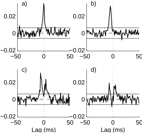
Figure 2 illustrates the bivariate time domain analysis between the firing sequences of neurons 2 and 3. These figures were generated from a single sample record of du-ration 100 seconds. The firing rate of all neurons varied from 10.5 - 18 spikes/sec, and the coefficient of variation varied from 0.69 - 0.78, over the four examples illustrated. The four estimates in figure 2 show the estimated bivariate correlation, ˆρ32(τ), between neurons 2 and 3, with neuron
2 the reference. Configuration a) has no connection be-tween neurons 2 and 3, however, the common input does
induce an apparent correlation between the two neurons. This is seen as a significant peak centred around time zero. Configurations b) - d) have the same pattern of common inputs as configuration a), except with an additional delay of 5 ms from 1→2 which induces an apparent direction-ality from 2 ← 3. This is observed as the peak in the unconditional estimate ˆρ32(τ) at negative values of lag τ
in figures 2b-2d. Configurations c) and d) also have excita-tory connections from 2→3 this appears as an additional peak in ˆρ32(τ) at positive values ofτ in figures 2c and 2d.
Configuration d) has an additional inhibitory connection from 2 ←3, we would expect to see a depression at neg-ative lags in figure 2d, however there is little evidence of this as it is masked by the apparent excitatory association induced by the common input from neuron 1. Thus the unconditional directionality analysis does not provide an accurate indication of the interactions between neurons 2 and 3.
−50 0 50
−0.02 0 0.02
a)
−50 0 50
−0.02 0 0.02
b)
−50 0 50
−0.02 0 0.02
c)
Lag (ms)
−50 0 50
−0.02 0 0.02
d)
[image:7.595.314.545.312.530.2]Lag (ms)
Figure 2: Bivariate directionality analysis for interactions between neurons 2 and 3. Configurations as shown in figure 1. Plots show the estimated correlation function, ˆρ32(τ), along with null value (dashed horizontal line at zero) and upper and lower 95% confidence limits (solid horizontal lines) based on the assumption of uncorrelated pro-cesses. The lag ranges are the same for all panels, a dotted vertical line atτ= 0 is included for reference.
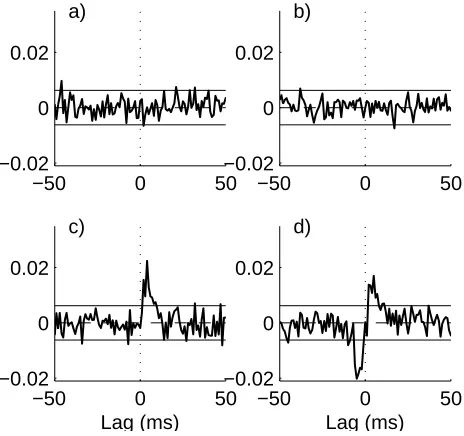
Figure 3 shows the estimated conditional correlation function, ˆρ32|1(τ), here the interaction between neurons 2
[image:7.595.70.258.404.567.2]fig 3c has a significant peak at positive lags in ˆρ32|1(τ), in
agreement with fig 1c. Configuration d) has an excitatory connection from 2→3 and an inhibitory connection from 2 ← 3. Both these are connections are accurately cap-tured by the estimate in fig 3d, in particular removal of the common input to neurons 2 and 3 has unmasked the inhibitory connection (compare fig 3d with fig 2d), there is now a clear, significant depression at negative time lags in ˆρ32|1(τ) in figure 3d.
−50 0 50
−0.02 0 0.02
a)
−50 0 50
−0.02 0 0.02
b)
−50 0 50
−0.02 0 0.02
c)
Lag (ms)
−50 0 50
−0.02 0 0.02
d)
[image:8.595.314.547.79.160.2]Lag (ms)
Figure 3: Conditional directionality analysis for interactions between neurons 2 and 3, conditioned on neuron 1. Configurations as shown in figure 1. Plots show the estimated conditional correlation func-tion, ˆρ32|1(τ), along with null value (dashed horizontal line at zero)
and upper and lower 95% confidence limits (solid horizontal lines) based on the assumption of uncorrelated processes. The lag ranges are the same for all panels, the vertical axes are the same as the corresponding plot in figure 2. A dotted vertical line at τ = 0 is included for reference.
3.2. Application to time series with known correlation struc-ture
This section considers application of the conditional di-rectionality metrics and functions to simulated time series data. The data are generated using combinations of white noise, from iid N(0,1), with known weights and delays. The first set consists of three random processes, where the bivariate correlation betweenxandyis entirely due to the common effects of processz, used as predictor in the condi-tional direccondi-tionality analysis. The results are summarised in Table 1 which gives the theoretical (target) values for
R2
yx, the mean and range (mean±2 SD) of the estimates
ˆ
R2
yx and ˆR2yx|z. Values were estimated from 100
indepen-dent trials, where each trial used 100 segments of length 210 samples.
The second set consists of a similar analysis, except in this case the theoretical (or target) conditional correlation,
R2
yx Rˆyx2 Rˆ2yx range Rˆ2yx|z Rˆyx2 |z range
0.1 0.108 0.105, 0.111 0.01 0.0091, 0.0110 0.3 0.305 0.301, 0.309 0.01 0.0092, 0.0110 0.5 0.502 0.500, 0.505 0.01 0.0092, 0.0110 0.7 0.700 0.698, 0.702 0.01 0.0092, 0.0107 0.9 0.899 0.899, 0.900 0.01 0.0092, 0.0110
Table 1: Theoretical values ofR2
yxand mean and range (mean±2SD) of ˆR2
yx and ˆR
2
yx|z for simulated time series where the correlation betweenxandyis due entirely to the common influence of process
z used as predictor in the conditional directionality analysis. The target value ofR2
yx|zis zero in all cases. Metrics calculated from 100 trials, each trial used 100 segments with 210
samples per segment.
R2
yx|z, differs from zero. The second set consists of a
simi-lar analysis, except in this case the theoretical (or target) conditional correlation, R2
yx|z, differs from zero. Here x
and y were generated from a mixture of Gaussian model as in Table 1, except two processes were common to bothx
andy, only one is the predictorz, thus the residual corre-lationR2
yx|zis non zero. The results are summarised in
Ta-ble 2 which also includes the target and estimated residual correlation, all configurations have non zero target values ofR2
yx and R2yx|z. The results in tables 1, 2 suggest that
estimates of the conditional directionality metric, R2 yx|z
can usefully distinguish direct interactions from common effects in multivariate time series.
R2
yx Rˆ2yx Rˆ2yx range R2yx|z Rˆyx2 |z Rˆ2yx|z range
0.4 0.403 0.399, 0.407 0.30 0.303 0.299, 0.308 0.4 0.403 0.399, 0.407 0.21 0.220 0.216, 0.224 0.5 0.502 0.498, 0.506 0.39 0.398 0.394, 0.402 0.5 0.502 0.498, 0.506 0.11 0.114 0.112, 0.117 0.6 0.601 0.598, 0.604 0.40 0.403 0.400, 0.406 0.6 0.601 0.598, 0.604 0.17 0.173 0.169, 0.176 0.8 0.800 0.798, 0.802 0.65 0.655 0.653, 0.658 0.8 0.800 0.798, 0.801 0.40 0.399 0.396, 0.402
Table 2: Theoretical values ofR2
yx(column 1) andR
2
yx|z(column 4) and mean and range (mean±2SD) of ˆR2
yx and ˆR
2
yx|z for simulated time series where the correlation betweenxandyis partly accounted for by the common influence of processzused as predictor in the con-ditional directionality analysis. Metrics calculated from 100 trials, each trial used 100 segments with 210
samples per segment.
The results presented in Table 2 use an instantaneous mixing of signals to generate the dependencies, thus co-herence, directional coherence and conditional directional coherence estimates are constant at all frequencies. In-troduction of delays into the generation of the processes
x and y will modulate the bivariate relationship across frequency, which should be removed in the conditional es-timates. The next example considers this scenario using two random processes generated according to the model:
x(t) = a1z1(t−1) +a2z2(t) + p
1−(a2
[image:8.595.46.278.208.426.2]0 0.5 0
0.5 1 a)
|Rˆyx(λ)|2
0 0.5
0 0.5 1
Frequency c)|Rˆ′yx;
−(λ)|
2
|Rˆ′yx;+(λ)|2
0 0.5
0 0.5
1 b)
|Rˆ′yx|z 1;+(λ)|
2
0 0.5
0 0.5 1
Frequency d)
|Rˆ′yx|z 2;−(
[image:9.595.52.270.84.303.2]λ)|2
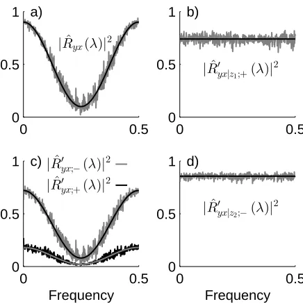
Figure 4: Conditional and unconditional directionality analyses of the relationship between four simulated processes, z1, z2 (predic-tors) and x,y. a) Estimated ordinary coherence between x andy
(grey) compared with theoretical model (black). b) Estimated for-ward component of conditional coherence estimate withz1 as
pre-dictor (grey) compared with theoretical model (black). c) Estimated forward (black) and reverse (grey) components of coherence estimate in panel a). The theoretical values are shown in grey and black for forward and reverse estimates, respectively. d) Estimated reverse component of conditional coherence estimate with z2 as predictor (grey) compared with theoretical model (black). Plots are shown against fractional frequency where 0.5 corresponds to the Nyquist frequency. See text for parameters and further details.
y(t) =a1z1(t) +a2z2(t−1) + p
1−(a2
1+a22)ε2(t), where
the four random processesz1,z2,ε1andε2are iidN(0,1),
and (a2
1+a22)<1. The coherence is|Ryx(λ)|2 =a41+a42+
2a2
1a22cos(2λ), hereλis radian frequency. The directional
components are|R′
yx;−(λ)|2=a41 a41+a42 −1
|Ryx(λ)|2and |R′
yx;+(λ)|2 = a42 a41+a42 −1
|Ryx(λ)|2, these can be
de-rived from (Halliday, 2015, eq (2.18), (2.20)). The two partial coherence estimates are|Ryx|z1(λ)|
2=a4
2(1−a21)−2
and|Ryx|z2(λ)|
2=a4
1(1−a22)−2, respectively. This
exam-ple should demonstrate an unmasking effect in the partial coherence estimates, which are constant over frequency, compared with the ordinary coherence which is modu-lated over frequency. Figure 4 illustrates analysis of a single trial, using 100 segments of length 210 points
gen-erated using this model forxandy with parametersa1= q
2/3√0.9 anda2= q
1/3√0.9.
For these parameters the coherence at zero frequency is |Ryx(0)|2 = 0.9. The two partial coherence functions
are |Ryx|z1(λ)|
2 = 0.74 and
|Ryx|z2(λ)|
2 = 0.855,
inde-pendent of frequency. The differential delays used in the generation of x(t) andy(t) will induce directionality into the pattern of dependencies. Common inputz1 influences
y before xthus induces directionality x←y, in contrast
common input z2 induces directional interaction x → y.
Thus the ordinary coherence should have components in the forward and reverse direction and we would expect to see non zero |Rˆ′
yx;+(λ)|2 and |Rˆ′yx;−(λ)|2. In the
condi-tional case the residual correlation after removal ofz1will
be in the forward direction , x → y, thus |Rˆ′
yx|z1;+(λ)|
2
should agree with |Ryx|z1(λ)|
2. The residual correlation
after removal ofz2will be in the reverse direction ,x←y,
thus|Rˆ′
yx|z2;−(λ)|2 should agree with |Ryx|z1(λ)|2.
The results in figure 4 are in good agreement with these expectations. Fig 4a shows the ordinary coherence esti-mate (grey) against the theoretical curve (black). There is good agreement. The other three panels explore how the non parametric directionality measures capture the uncon-ditional and conuncon-ditional relationship betweenxandy. Fig 4c shows the two bivariate directionality estimates, for-ward |Rˆ′
yx;+(λ)|2 (black), and reverse |Rˆ′yx;−(λ)|2 (grey).
These two estimates sum to give the coherence estimate in fig 4a. Both estimates agree with the theoretical di-rectional components shown superimposed on each trace. The induced interaction is stronger in the reverse direc-tion, since a1 > a2 in the above time series model.
Fig-ure 4b shows the constant theoretical |Ryx|z1(λ)|2, 0.74
(black) and the estimated conditional forward coherence estimate |Rˆ′
yx|z1;+(λ)|2 (grey). There is good agreement
between these two, the other estimated directional compo-nents,|Rˆ′
yx|z1;−(λ)|2 and|Rˆyx′ |z1;0(λ)|2 are negligible (not
shown). Similarly in fig 4d there is good agreement be-tween the theoretical|Ryx|z2(λ)|2= 0.855 (black) and the
estimated|Rˆ′
yx|z2;−(λ)|2 (grey), where the conditional
di-rectional analysis correctly identifies the interaction in the reverse direction. The other estimated directional compo-nents|Rˆ′
yx|z2;+(λ)|
2 and |Rˆ′
yx|z2;0(λ)|
2 are negligible (not
shown). Thus, the unconditional and conditional direc-tionality analysis is able to correctly infer the strength and direction between the four simulated processesz1,z2,
xand y.
3.3. Application to bilateral Hippocampal in vivo record-ings - Bivariate directionality analysis
approval and were carried out in accordance with the An-imals (Scientific Procedures) Act 1986, UK.
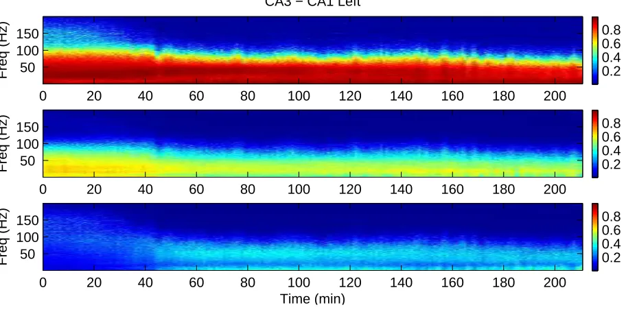
The approach is applied to a single record of dura-tion 211 minutes. Here we consider bivariate direcdura-tion- direction-ality analysis between simultaneous LFP records in CA1 and CA3 hippocampal regions in each hemisphere. Fig-ure 5 shows the estimated coherence (|Rˆyx(λ)|2, top) and
the forward (|Rˆ′
yx;+(λ)|2, middle) and reverse (|Rˆ′yx;−(λ)|2,
lower) components for CA3-CA1 in left hemisphere. Fig-ure 6 shows the estimates for CA3-CA1 in the right hemi-sphere, in both cases CA3 region is the reference. The complete record was split into blocks for analysis, these blocks consisted of 58 segments of length 1024 points. Each block was analysed separately and bivariate direc-tionality parameters calculated as described in Halliday (2015). Adjacent blocks were non-overlapping. Each block is approximately 1 minute in duration, 59.39 sec, with sam-pling rate 1ms.
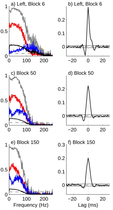
Both sets demonstrate strong coherence between CA3 and CA1 LFP signals, and exhibit a modulation of the co-herence and the directional components after application of KA. Both the strength of coherence and range of fre-quencies change after KA is applied. This can be seen more clearly in the sections illustrated in figures 7 and 8. These illustrate the frequency (left) and time domain (right) bi-variate directionality analysis for fixed blocks 6 (top; pre KA injection), 50 (middle; soon after KA injection) and 150 (lower; well after KA injection), respectively, corre-sponding to ∼1 minute blocks centred at 5.4, 49 and 148 minutes into the data set. These figures represent vertical sections through the time-frequency plots in figs 5 and 6, at fixed times.
For the left (ipsilateral) side the overall strength of teraction between CA3 and CA1 decreases after local in-jection of KA. The range of frequencies that exhibit signif-icant coherence decreases from 200 Hz (block 6) to 125 Hz and 115Hz (blocks 50 and 150, respectively). The inter-action tends to become more balanced, the percentage of
ˆ
R2
yx;200, the overall strength of correlation at frequencies
up to 200 Hz, in the forward direction remains constant at 54%, the percentage in the reverse direction increases from 22% in block 6 to 32% in block 50 and 36% in block 150, accompanied by a decrease in the percentage at zero lag. For this data, the frequencies where the directional com-ponents are strongest are not those where the original co-herence is strongest. For the left side, the forward compo-nent (red) peaks at lower frequencies, whereas the reverse component (blue) peaks at higher frequencies than the or-dinary coherence. In block 6 the oror-dinary coherence peaks around 30 Hz, the forward component peaks around 20 Hz and the reverse component peaks at frequencies>100Hz. In block 150 the coherence and forward component have peaks at similar frequencies to block 6, whereas the reverse component has a peak around 50 Hz.
Injection of local KA into the left hemisphere also mod-ulates the interaction between the CA3 and CA1 LFP
sig-nals in the right hemisphere as shown by the sections in figure 8. The range of frequencies that exhibit significant coherence decreases from 110 Hz (block 6) to 85 Hz and 75Hz (blocks 50 and 150, respectively). The interaction tends to become more one directional, the percentage of
ˆ
R2
yx;200, in the forward direction increases from 67% in
block 6 to 86% in block 50 and 90% in block 150. For the right side in block 6 the coherence and forward com-ponents both have peaks around 30 Hz, in contrast the reverse component has a peak around 50 Hz. In later sec-tions the magnitude of the reverse component is greatly reduced thus the forward component is very similar to the ordinary coherence, in block 150 the maximum is around 20 Hz.
The time domain estimates (right column) gives further insight into the characteristics of the interaction between CA3 and CA1. The positive peak in ˆρyx(τ) indicates a
latency of around 3-4 ms from CA3→CA1. In the basal section (block 6) an interaction can be seen in the oppo-site direction, CA3←CA1, this has a similar latency of around 3 ms. Interestingly this feature has negative mag-nitude (fig 8b, negative lag) suggestive of an inhibitory effect. The application of KA abolished this CA3←CA1 interaction in the contralateral HPC (fig 8d, f). The re-sults demonstrate that unilateral local KA injection has a marked effect on the strength and directionality of inter-action between CA3 and CA1 in both left and right HPC. The KA appears to have different effects on each hemi-sphere, the strength of CA3←CA1 interaction increases in the ipsilateral (left) hemisphere (Figure 7, blue lines), whereas it reduces in the contralateral (right) hemisphere (Figure 8, blue lines). These effects persist for the duration of the available record, 3 hours post injection.
4. Discussion
This article presents two important developments to the non parametric directionality framework in Halliday (2015). The first is the development of conditional di-rectionality measures, the second considers applicability to time series data. Conditional measures are derived by decomposing the MMSE pre-whitened (Eldar and Oppen-heim, 2003) partial coherence in the same manner as the unconditional measures decompose the ordinary coherence (Halliday, 2015). The MMSE pre-whitening step ensures equality between the partial cross spectrum and partial co-herence, equation 17, allowing the conditional scalar mea-sure of dependence, R2
yx|z, to be determined by
integra-tion of the pre-whitened partial cross spectrum fw yx|z(λ),
equation 18. Estimates of this, and the decomposition into three directional components,R2
yx|z;−,R2yx|z;0andR2yx|z;+,
provide scalar measures of linear association, on a scale from 0 to 1, of the interaction between processes (x, y) af-ter taking into account any common linear influence from process z. An additional set of functions, |R′
yx|z;−(λ)|2,
|R′
co-0.2 0.4 0.6 0.8
Freq (Hz)
CA3 − CA1 Left
0 20 40 60 80 100 120 140 160 180 200
150 100 50
0.2 0.4 0.6 0.8
Freq (Hz)
0 20 40 60 80 100 120 140 160 180 200
150 100 50
0.2 0.4 0.6 0.8
Time (min)
Freq (Hz)
0 20 40 60 80 100 120 140 160 180 200
[image:11.595.73.529.108.337.2]150 100 50
Figure 5: Bivariate directionality analysis of LFP recordings from CA3 and CA1 in left hippocampus in an anaesthetised rat. Kainic acid was injected locally into the left hippocampus at 30 minutes. The plots show the estimated coherence (top) and forward (CA3→CA1, middle) and reverse (CA3←CA1, bottom) components, with CA3 as the reference. Analysis was undertaken by splitting the complete record in to non-overlapping blocks of duration approximately 1 minute. Scale bars on the right indicate the strength of coherence (top) and directional (middle, bottom) components, all to the same scale. The 95% significance level for the coherence estimate (top) is 0.0512, based on the assumption of uncorrelated signals.
0.2 0.4 0.6 0.8
Freq (Hz)
CA3 − CA1 Right
0 20 40 60 80 100 120 140 160 180 200
150 100 50
0.2 0.4 0.6 0.8
Freq (Hz)
0 20 40 60 80 100 120 140 160 180 200
150 100 50
0.2 0.4 0.6 0.8
Time (min)
Freq (Hz)
0 20 40 60 80 100 120 140 160 180 200
150 100 50
[image:11.595.71.528.461.690.2]0 100 200 0
0.5
1 a) Left, Block 6
0 100 200
0 0.5
1 c) Block 50
0 100 200
0 0.5 1
Frequency (Hz) e) Block 150
−20 0 20
0 0.1 0.2
b) Left, Block 6
−20 0 20
0 0.1 0.2
d) Block 50
−20 0 20
0 0.1 0.2 0.3
Lag (ms) f) Block 150
Figure 7: Directionality analysis for 1 minute blocks centred at 5.4 (block 6, top), 49 (block 50 centre) and 148 minutes (block 150 lower). Analysis is for CA3-CA1 interaction in left hemisphere (CA3-CA1 L), ipsilateral to local KA injection. Left column shows fre-quency domain analysis, with coherence (grey), forward component (red) reverse component (blue) and zero lag component (black). The dashed horizontal line is the estimated upper 95% confidence limit for the coherence based on the assumption of uncorrelated signals. Right column illustrates time domain analysis showing estimated correlation function, along with null value (dashed horizontal line) and upper and lower 95% confidence limits based on the assumption of uncorrelated signals. Further discussion in text.
herence summatively into reverse, zero lag, and forward components, equation 26, in an analogous manner to that for the ordinary coherence in Halliday (2015). A comple-mentary time domain partial correlation function,ρyx|z(τ)
provides a time domain view of the conditional dependence betweenxandy with predictorz.
The concept of partial coherence is not new (Tick, 1963), it has been used as a technique to infer neuronal connectivity that can distinguish common inputs from
di-0 100 200
0 0.5
1 a) Right, Block 6
0 100 200
0 0.5
1 c) Block 50
0 100 200
0 0.5 1
Frequency (Hz) e) Block 150
−20 0 20
−0.05 0 0.05 0.1
b) Right, Block 6
−20 0 20
−0.05 0 0.05 0.1
d) Block 50
−20 0 20
−0.05 0 0.05 0.1
Lag (ms) f) Block 150
Figure 8: Directionality analysis for 1 minute blocks centred at 5.4 (block 6, top), 49 (block 50 centre) and 148 minutes (block 150 lower). Analysis is for hippocampal CA3-CA1 interaction in the right hemisphere (CA3-CA1 R), contralateral to local KA injection. Layout, format and confidence limits same as in figure 7. Further discussion in text.
[image:12.595.53.275.85.498.2] [image:12.595.311.527.106.516.2]Brillinger (1974); Halliday et al. (1995). The relationship between our non-parametric approach and parametric and other non-parametric approaches is discussed in Halliday (2015), these comments also apply to the conditional case considered here. The results using simulated data in ta-bles 1 and 2 demonstrate that the unconditional and con-ditional non parametric directionality measures correctly infer the relationship between simulated time series signals generated from mixtures of Gaussians. Partial coherence analysis of spike train data using up to 7 predictors, and of human EEG using up to 8 predictors is presented in Halliday (2005) and Medkour et al. (2009), respectively. Partial coherence analysis of neural spike trains can distin-guish between direct and indirect connections, increasing numbers of predictors can give a more accurate representa-tion of synaptic interacrepresenta-tions (Eichler et al., 2003). Future work will consider how the MMSE pre-whitening step can be extended to allow partial coherence estimates of order greater than 1 to be decomposed by direction.
The framework is applied to experimental times se-ries data using LFP records from bilateral hippocampus in anaesthetised rat. Figures 5 and 6 show how the direc-tionality changes over the 211 minute record in response to local injection of kainic acid to induce epileptiform ac-tivity after 30 minutes. Figures 7 and 8 illustrate a bi-variate directionality analysis at fixed points before and after application of kainic acid and demonstrate system-atic changes in the pattern and direction of interaction between CA1 and CA3 LFP signals in each hemisphere in response to drug injection. Changes in overall correlation and directionality can be quantified if necessary using the scalar metrics defined in equation 22. A more detailed analysis of this data will be presented elsewhere including non parametric conditional analysis of the intra and inter hemispheric interactions.
In this paper we have introduced a non parametric ap-proach to estimate conditional directionality. The analysis decomposes the partial coherence by direction of interac-tion, providing a set of scalar measures which decompose the conditional correlation,R2
yx|z, summatively into three
components: R2
yx|z;−,R2yx|z;0andRyx2 |z;+representing the
components in the reverse, zero lag and forward directions, respectively. The estimated partial coherence, |Rˆyx|z(λ)|2
is decomposed summatively into three directional compo-nents: |Rˆ′
yx|z;−(λ)|2, |Rˆ′yx|z;0(λ)|2 and|Rˆyx′ |z;+(λ)|2. The
framework includes complementary time and frequency domain measures. The time domain function, ρyx|z(τ),
which is free from within variable effects, provides a direct indication of the directionality between processes (x, y) af-ter removal of the common effects of processz.
Our framework has applicability to both time series and spike train data. As advances in multielectrode array recordings generate ever larger multivariate data sets with LFP and single unit recordings there is a need for appro-priate signal processing tools to infer network dynamics. The novel non parametric method presented here has the
flexibility to combine spike train and time series data in a single framework, and is free from any concerns regarding the use of low order auto regressive models to represent electrophysiological signals. The framework should have broad application to a wide range of data including human electroencephalography (EEG) and magnetoencephalogra-phy (MEG).
5. Acknowledgements
MHS is funded by The Ministry of Higher Education, Malaysia.
6. Software
A software toolbox in MATLAB to undertake the anal-ysis in this paper is available for free download. The soft-ware includes a user guide and example scripts. It is avail-able from: http://www.neurospec.org/
Appendix A. Algorithmic descriptions for two and three variable cases.
This appendix includes algorithmic level descriptions of the two variable (Halliday, 2015),R2yx, and three
vari-able, R2
yx|z, analyses and their related quantities:
direc-tional metrics, frequency domain functions and time do-main functions. The data vectors are assumed to have lengthR, where R=LT, the analysis uses only complete segments. The first step in both cases is the calculation of the discrete Fourier transform of the disjoint sections of lengthT over allLsegments. This is indicated in line 3 of Algorithm 1 and line 3 of Algorithm 2 with the statement - Calculate: dT
x(λ, l),. . .. Summations are indicated using
the notation sum{·}, where necessary the range of the in-dex is indicated after this, for example, allτ in line 16, or
τ <0 in line 17 of Algorithm 1. Forward and inverse dis-crete Fourier transforms calculated with an fft algorithm are indicated using the notation fft{·} and ifft{·}, respec-tively. Any reduced range in the independent variable is indicated using the same notation as the summation, for example,τ <0 in line 20 of Algorithm 1 indicates an FFT calculated using only negative values of τ, but using the same Fourier frequencies, all discrete Fourier transforms have lengthT, using zero padding where necessary. These algorithm descriptions follow the convention in MATLAB with respect to scaling factors in forward and reverse fft algorithms, namely a factor ofT−1 is associated with the
reverse transform, no scaling factor is included in the for-ward transform.
References
Algorithm 1Unconditional directionality: R2 yx
Input: x, y,T
Output: Metrics: ˆRyx2 , ˆR2yx;−, ˆR2yx;0, ˆR2yx;+
Output: Frequency domain: |Rˆyx(λ)|2, |Rˆ′yx;−(λ)|2,
|Rˆ′
yx;0(λ)|2,|Rˆyx′ ;+(λ)|2
Output: Time domain: ˆρyx(τ)
1: L←R/T
2: forl= 1toLdo 3: Calculate dFT:dT
x(λ, l),dTy(λ, l)
4: end for
5: fˆxx(λ)←(2πLT)−1×sum|dTx(λ, l)|2 ,l= 1. . . L
6: fˆyy(λ)←(2πLT)−1×sum|dTy(λ, l)|2 ,l= 1. . . L
7: wˆxx(λ)←fˆxx(λ)−1/2
8: wˆyy(λ)←fˆyy(λ)−1/2
9: forl= 1toLdo 10: dwT
x(λ, l)←dTx(λ, l)×wˆxx(λ)
11: dwT
y(λ, l)←dTy(λ, l)×wˆyy(λ)
12: end for 13: fˆw
yx(λ) ← (2πLT)
−1
× sumndwT
y(λ, l)×dwxT(λ, l) o
,
l= 1. . . L
14: |Rˆyx(λ)|2← |fˆyxw(λ)|2
15: ρˆyx(τ)←ifft n
ˆ
fw yx(λ)
o
16: Rˆ2
yx←sum
ˆ
ρyx(τ)2 , allτ
17: Rˆ2yx;−←sumρˆyx(τ)2 ,τ <0
18: Rˆ2 yx;0←
ˆ
ρyx(0)2
19: Rˆ2yx;+←sum
ˆ
ρyx(τ)2 ,τ >0
20: fˆ′
yx;−(λ)←fft{ρˆyx(τ)},τ <0
21: fˆyx′ ;0(λ)←ρˆyx(0)
22: fˆ′
yx;+(λ)←fft{ρˆyx(τ)},τ >0
23: Syx(λ)← |fˆyx′ ;−(λ)|2+|fˆyx′ ;0(λ)|2+|fˆyx′ ;+(λ)|2
24: |Rˆ′
yx;−(λ)|2←
|fˆ′
yx;−(λ)|2/Syx(λ)
× |Rˆyx(λ)|2
25: |Rˆ′
yx;0(λ)|2←
|fˆ′
yx;0(λ)|2/Syx(λ)
× |Rˆyx(λ)|2
26: |Rˆ′
yx;+(λ)|2←
|fˆ′
yx;+(λ)|2/Syx(λ)
× |Rˆyx(λ)|2
Brillinger DR (1974) Fourier analysis of stationary processes. Pro-ceedings of the IEEE. 62: 1628-1643.
Brillinger DR (1975) Time Series - Data Analysis and Theory. Holt Rinehart & Winston Inc. New York.
Brillinger DR (1988) Some statistical methods for random process data from seismology and neurophysiology. Annals of statistics, 16: 1-54.
Chen Y, Bressler SL, Ding M (2006) Frequency decomposition of con-ditional Granger causality and application to multivariate neural field potential data. Journal of neuroscience methods, 150: 228-237.
Chicharro D (2012) On the spectral formulation of Granger causality. Biological cybernetics, 105: 331-347.
Conway BA, Halliday DM, Rosenberg JR (1993). Detection of weak synaptic interactions between single Ia-afferents and motor-unit spike trains in the decerebrate cat. Journal of Physiology, 471, 379-409
Coomber B, O’Donoghue MF, Mason R (2008) Inhibition of endo-cannabinoid metabolism attenuates enhanced hippocampal neu-ronal activity induced by kainic acid. Synapse, 62: 746-755.
Algorithm 2Conditional directionality: R2 yx|z
Input: x, y, z,T Output: Metrics: ˆR2
yx|z, ˆR 2
yx|z;−, ˆR
2 yx|z;0, ˆR
2 yx|z;+
Output: Frequency domain: |Rˆyx|z(λ)|2, |Rˆ′yx|z;−(λ)|2, |Rˆ′
yx|z;0(λ)| 2,
|Rˆ′
yx|z;+(λ)| 2
Output: Time domain: ˆρyx|z(τ)
1: L←R/T
2: forl= 1to Ldo
3: Calculate: dTx(λ, l),dyT(λ, l),dTz(λ, l) 4: end for
5: fˆzz(λ)←(2πLT)−1×sum|dTz(λ, l)|2 ,l= 1. . . L
6: fˆxz(λ) ← (2πLT)−1× sum n
dT
x(λ, l)×dTz(λ, l) o
, l = 1. . . L
7: fˆyz(λ) ← (2πLT)−1× sum n
dT
y(λ, l)×dTz(λ, l) o
, l = 1. . . L
8: forl= 1to Ldo 9: dT
x|z(λ, l)←dTx(λ, l)−
ˆ
fxz(λ)/fˆzz(λ)
×dT z(λ, l)
10: dT
y|z(λ, l)←dTy(λ, l)−
ˆ
fyz(λ)/fˆzz(λ)
×dT z(λ, l)
11: end for
12: fˆxx|z(λ)←(2πLT)−1×sum n
|dT
x|z(λ, l)|2 o
,l= 1. . . L 13: fˆyy|z(λ)←(2πLT)−1×sum
n |dT
y|z(λ, l)|2 o
,l= 1. . . L 14: wˆxx|z(λ)←fˆxx|z(λ)−1/2
15: wˆyy|z(λ)←fˆyy|z(λ)−1/2
16: forl= 1to Ldo 17: dwT
x|z(λ, l)←dTx|z(λ, l)×wˆxx|z(λ)
18: dwT
y|z(λ, l)←dTy|z(λ, l)×wˆyy|z(λ)
19: end for 20: fˆw
yx|z(λ) ← (2πLT)
−1 ×
sumndwT
y|z(λ, l)×dwxT|z(λ, l) o
,l= 1. . . L 21: |Rˆyx|z(λ)|2← |fˆyxw|z(λ)|2
22: ρˆyx|z(τ)←ifft n
ˆ
fw yx|z(λ)
o
23: Rˆ2
yx|z←sum
ˆ
ρyx|z(τ)2 , allτ
24: Rˆ2
yx|z;−←sum
ˆ
ρyx|z(τ)2 ,τ <0
25: Rˆ2yx|z;0←ρˆyx|z(0)2
26: Rˆ2yx|z;+←sumρˆyx|z(τ)2 ,τ >0
27: fˆ′
yx|z;−(λ)←fft
ˆ
ρyx|z(τ) ,τ <0
28: fˆ′
yx|z;0(λ)←ρˆyx|z(0)
29: fˆ′
yx|z;+(λ)←fft
ˆ
ρyx|z(τ) , τ >0
30: Syx|z(λ)← |fˆyx′ |z;−(λ)|2+|fˆyx′ |z;0(λ)|2+|fˆyx′ |z;+(λ)|2
31: |Rˆ′yx|z;−(λ)|2 ←
|fˆ′
yx|z;−(λ)|
2/S yx|z(λ)
× |Rˆyx|z(λ)|2
32: |Rˆ′
yx|z;0(λ)|2←
|fˆ′
yx|z;0(λ)|2/Syx|z(λ)
× |Rˆyx|z(λ)|2
33: |Rˆ′
yx|z;+(λ)|2←
|fˆ′
yx|z;+(λ)|2/Syx|z(λ)
× |Rˆyx|z(λ)|2
Dhamala M, Rangarajan G, Ding M (2008a) Analyzing information flow in brain networks with nonparametric Granger causality. Neu-roImage, 41: 354-362.
Dhamala M, Rangarajan G, Ding M (2008b) Estimating Granger Causality from Fourier and Wavelet Transforms of Time Series Data. Physical Review Letters, 100: 18701.
Eichler M, Dahlhaus R, Sandkuhler J (2003) Partial correlation anal-ysis for the identification of synaptic connections. Biological cy-bernetics, 89: 289-302.
Eldar YC, Oppenheim AV (2003) MMSE whitening and subspace whitening. IEEE Transactions on Information Theory, 49: 1846-1851.
Ezekiel M, Fox KA (1958) Methods of correlation and regression analysis, 3rd ed. John Wiley, New York.
Gersch W (1972) Causality or driving in electrophysiological signal analysis. Mathematical Biosciences, 14: 177-196.
Geweke JF (1982) Measurement of Linear Dependence and Feedback Between Multiple Time Series. Journal of the American Statistical Association, 77: 304-324
Geweke JF (1984) Measures of conditional linear dependence and feedback between time series. Journal of the American Statistical Association, 79: 907-915.
Granger CWJ (1969) Investigating Causal Relations by Econometric Models and Cross-spectral Methods. Econometrica, 37: 424-438. Guo S, Seth AK, Kendrick KM, Zhou C, Feng J (2008). Partial
Granger causality–eliminating exogenous inputs and latent vari-ables. Journal of Neuroscience Methods, 172(1), 7993.
Halliday DM, Rosenberg JR, Amjad AM, Breeze P, Conway BA, Farmer SF (1995) A framework for the analysis of mixed time se-ries/point process data - Theory and application to the study of physiological tremor, single motor unit discharges and electromyo-grams. Progress in Biophysics and molecular Biology, 64: 237-278. Halliday DM (2005) Spike-train analysis for neural systems. In: Reeke GN, Poznanski RR, Lindsay KA, Rosenberg JR, Sporns O, editors. Modeling in the neurosciences. 2nd ed. Taylor & Francis pp 555-579.
Halliday DM (2015) Non parametric directionality measures for point process and time series data. Journal of Integrative Neuroscience, 14(2) 253-277.
Kaiser M (2011), A tutorial in connectome analysis: Topological and spatial features of brain networks, NeuroImage, 57: 892-907. Kaminski M, Ding M, Truccolo WA, Bressler SL (2001)
Evaluat-ing causal relations in neural systems: Granger causality, directed transfer function and statistical assessment of significance. Biolog-ical Cybernetics, 85: 145-157.
Lindsay KA, Rosenberg JR (2011) Identification of directed interac-tions in networks. Biological cybernetics, 104: 385-396.
Medkour T, Walden AT, Burgess A (2009) Graphical modelling for brain connectivity via partial coherence. Journal of neuroscience methods, 180: 374-383.
Newman M (2010) Networks: An Introduction (p. 720). Oxford Uni-versity Press, UK.
Percival DB, Walden AT (1993) Spectral Analysis for Physical Ap-plications. Cambridge Univ. Press, UK.
Pierce DA (1979) R2 Measures for Time Series. Journal of the Amer-ican Statistical Association, 74: 901-910.
Pierce DA (1982) Comment on Geweke paper. Journal of the Amer-ican Statistical Association, 77: 315-316.
Priestley MB (1981) Spectral analysis and time series. Academic Press, London.
Rosenberg JR, Amjad A, Breeze P, Brillinger DR, Halliday DM (1989). The Fourier approach to the identification of functional coupling between neuronal spike trains. Progress in Biophysics and Molecular Biology, 53: 1-31.
Rosenberg JR, Halliday DM, Breeze P, Conway BA (1998). Identi-fication of patterns of neuronal connectivitypartial spectra, par-tial coherence, and neuronal interactions. Journal of Neuroscience Methods, 83: 57-72.
Rubinov M, Sporns O (2010) Complex network measures of brain connectivity: Uses and interpretations. NeuroImage, 52: 1059-1069.
Salvador R, Suckling J, Schwarzbauer C, Bullmore E (2005) Undi-rected graphs of frequency-dependent functional connectivity in whole brain networks. Philosophical transactions of the Royal So-ciety of London. Series B, Biological sciences, 360: 937-946. Schelter B, Winterhalder M, Eichler M, Peifer M, Hellwig B,
Guschlbauer B, Lucking CH, Dahlhaus R, Timmer J (2006) Test-ing for directed influences among neural signals usTest-ing partial di-rected coherence. Journal of neuroscience methods, 152: 210-219. Senik MH, O’Donoghue MF, Mason R (2013) Intra- and inter-hippocampal connectivity in a KA-induced mTLE rat model. Pro-gram No 143.05. 2013 Neuroscience Meeting Planner. San Diego, California: Society for Neuroscience, 2013. Online.
Thomson DJ, Chave A (1991) Jackknifed error estimates for spectra, coherences, and transfer functions. In S. Haykin (Ed.), Advances in spectrum analysis and array processing, 1. pp 58-113. Tick LJ (1963) Conditional spectra, linear systems and coherency.
In: Time series analysis, Ed Rosenblatt M, Wiley, New-York, 197-203.