slab
.
White Rose Research Online URL for this paper:
http://eprints.whiterose.ac.uk/114291/
Version: Accepted Version
Article:
Ballai, I., Pinter, B., Oliver, R. et al. (1 more author) (2017) Dissipative instability in a
partially ionised prominence plasma slab. Astronomy & Astrophysics. ISSN 0004-6361
https://doi.org/10.1051/0004-6361/201629215
Reproduced with permission from Astronomy & Astrophysics, © ESO.
[email protected] https://eprints.whiterose.ac.uk/ Reuse
Unless indicated otherwise, fulltext items are protected by copyright with all rights reserved. The copyright exception in section 29 of the Copyright, Designs and Patents Act 1988 allows the making of a single copy solely for the purpose of non-commercial research or private study within the limits of fair dealing. The publisher or other rights-holder may allow further reproduction and re-use of this version - refer to the White Rose Research Online record for this item. Where records identify the publisher as the copyright holder, users can verify any specific terms of use on the publisher’s website.
Takedown
If you consider content in White Rose Research Online to be in breach of UK law, please notify us by
Astronomy & Astrophysics manuscript no. maibro16˙final˙version˙2c c ESO 2017 March 23, 2017
Dissipative instability in a partially ionised prominence plasma slab
I. Ballai
1,2, B. Pint´er
3, R Oliver
4and M. Alexandrou
1,
1
Solar Physics and Space Plasma Research Centre (SP2
RC), Department of Applied Mathematics, The University of Sheffield, Sheffield, UK, S3 7RH, email:[email protected]
2
Konkoly Observatory, MTA Research Centre for Astronomy and Earth Sciences, Konkoly-Thege Mikl´os ´ut 15-17, 1121, Budapest, Hungary
3
Solar System Physics Research Group, Institute of Mathematics, Physics and Computer Sciences, Aberystwyth University, Penglais Campus, UK, email:[email protected]
4
Departament de F´ısica, Universitat de les Illes Balears, 07122 Palma de Mallorca, Spain, email:[email protected]
Received dd mmm yyyy / Accepted dd mmm yyyy
ABSTRACT
Aims.We aim to investigate the nature of dissipative instability appearing in a prominence planar thread filled with partially ionised plasma in the incompressible limit. The importance of partial ionisation is investigated in terms of the ionisation factor and the wavelength of sausage and kink waves propagating in the slab.
Methods.In order to highlight the role of partial ionisation, we have constructed models describing various situations we can meet in solar prominence fine structure. Matching the solutions for the transversal component of the velocity and total pressure at the interfaces between the prominence slab and surrounding plasmas, we derived a dispersion relation whose imaginary part describes the evolution of the instability. Results were obtained in the limit of weak dissipation. We have investigated the appearance of instabilities in prominence dark plumes using single and two-fluid approximations .
Results.Using simple analytical methods, we show that dissipative instabilities appear for flow speeds that are less than
the Kelvin-Helmholtz instability threshold. The onset of instability is determined by the equilibrium flow strength, the ionisation factor of the plasma, the wavelength of waves and the ion-neutral collisional rate. For a given wavelength and for ionisation degrees closer to a neutral gas, the propagating waves become unstable for a narrow band of flow speeds, meaning that neutrals have a stabilising effect. Our results show that the partially ionised plasma describing prominence dark plumes becomes unstable only in a two-fluid (charged particles-neutrals) model, that is for periods that are smaller than the ion-neutral collision time.
Conclusions.The present study improves our understanding of the complexity of dynamical processes and stability of
solar prominences and the role partial ionisation in destabilising the plasma. We showed the necessity of two-fluid approximation when discussing the nature of instabilities: waves in a single fluid approximation show a great deal of stability. Our results clearly show that the problem of partial ionisation introduces new aspects of plasma stability with consequences on the evolution of partially ionised plasmas and solar prominences, in particular.
Key words.Magnetohydrodynamics (MHD)—Sun: filaments, prominences—Sun: magnetic fields—Sun: instability
1. Introduction
The lower part of the solar atmosphere is a perfect example of an environment where temperatures are not high enough for a complete ionisation of the fluid and charged parti-cles and neutrals can coexist due to the collision between them. In particular, solar prominences are regions of cool and dense plasmas where the plasma is not fully ionised and the hydrogen ionisation degree could probably vary in dif-ferent prominences or even in difdif-ferent regions within the same prominence (Hirayama 1986, Patsourakos and Vial 2002). In this state, the role of neutrals becomes impor-tant as the source of momentum transfer between species. Since the neutrals are not controlled by the magnetic field, they flow inside the prominence, preventing the formation of any equilibrium that was not dynamic. Gilbert et al. (2007) found evidence for cross-field diffusion of neutrals that could explain the mass loss in quiescent prominences. The mathematical description of partially ionised gases is different from the standard magnetohydrodynamic (MHD) approach, as the equations needed to fully describe
the state and dynamics of the plasma have to contain corre-sponding equations for each species. Considerable advance-ment can be achieved if we suppose that the prominence plasma is made up from hydrogen only. In addition, we as-sume that the plasma is in ionisation equilibrium, that is the number of ionsation and recombination processes are balanced and the time required for an ion to recombine with an electron (or a neutral atom to ionise through colli-sion) is much shorter than any dynamical time scale under discussion (e.g. periods, damping times, etc.).
Although the partial ionisation of the prominence plasma would mean that each constituent species is treated separately, in the case of ionisation equilibrium and strong correlation of temperature between species, the plasma can still be treated as a single fluid and various quantities in the equations (e.g. density, pressure, etc.) are just the sum of partial components for each species. For periods that are shorter than the ion-neutral collisional frequency, the plasma dynamics has to be described within the framework of two-fluid MHD.
A necessary ingredient in our discussion is the equilib-rium flow that has a very strong observational evidence in prominences and nowadays they are observed in various spectral lines, such as Hα, UV/EUV (Labrosse et al. 2010).
Flow speeds range between 5-20 km s−1 in quiescent
fila-ments (Lin et al. 2003) to 15-46 km s−1 in active region
prominences, seen by Hinode/SOT (Okamoto et al. 2007). At the same time, complex dynamics containing vertical up-flows and downup-flows were observed by Berger et al. (2008) in limb prominences. Vorticities inside the prominence of sizes approximately of the order of 105×105 km2were
ob-served by Liggett and Zirin (1984) with rotation rates of 30 km s−1.
In our study we assume that the plasmas we are deal-ing with are non-ideal. Accorddeal-ing to the standard picture, dynamical processes taking place in these media will be af-fected by non-ideal mechanisms by lowering or amplifying their amplitude; as a result the energy stored in waves and oscillations are dissipated or accumulated. The plasmas un-der consiun-deration are dissipative with anisotropic viscosity in the solar corona, while the dynamics in the prominence plasma is affected by dissipative processes that are charac-teristic for its ionisation state.
It is well known that the collisions between ions and neutrals introduce an effective anisotropic resistivity into the single fluid equations (Cowling 1957; Braginskii 1965), called Cowling resistivity, which acts only on perpendicu-lar currents. Khodachenko et al. (2004) estimated that in the photosphere and chromosphere the magnitude of this resistivity is a few orders of magnitude larger than the clas-sical parallel Spitzer resistivity, for chromospheric parame-ters this difference is of the order of 104−105. The effect
of the Cowling resistivity was investigated in connection to wave damping (Goodman 2001, Leake et al. 2005, Forteza et al. 2008, Carbonell et al. 2010, Singh and Krishan 2010), flux emergence (Leake and Arber 2006, Arber et al. 2007), the formation of nonlinear force-free fields in the chromo-sphere from photospheric fields (Arber et al. 2009), or even reconnection (Ni et al. 2007).
The problem of the stability of plasmas, and promi-nences in particular, is a very important aspect of solar at-mospheric physics as instabilities can disrupt the magnetic configuration on large scales or can generate turbulent con-vection cells, which significantly enhance the transport of energy across magnetic surfaces. In general, these instabili-ties can be categorised in many ways. In the present study, however, we can classify them as ideal instabilities and non-ideal instabilities. In the first class, the source of instability (the reservoir for energy and momentum gain and growth) comes from currents or pressure gradients that are present in ideal plasmas. Particular examples of ideal instabilities are the Kelvin-Helmholtz (KH) and Rayleigh-Taylor (RT) instabilities, that have been studied in detail in hydrody-namics and MHD (e.g. Soler et al. 2012, Murawski et al. 2016, Oliver et al. 2016, etc. studied the triggering and evo-lution of the KH instabilities in prominence plasmas, while Diaz et al. 2012, Shadmehri et al. 2013, Diaz et al. 2014, Khomenko et al. 2014b, Ruderman 2015, etc. discussed the problem of RT instability in solar prominences).
On the other hand, non-ideal instabilities assume that the plasma contains some sort of transport mechanism that helps in the triggering of instability (e.g. dissipative insta-bility, thermal instainsta-bility, tearing mode instainsta-bility, etc.). In these instabilities the presence of a non-ideal effect is a
necessity. For instance, Hillier et al. (2010) studied the ef-fect of Cowling resistivity on the Kippenhahn and Schluter prominence model. They found that due to the inclusion of the Cowling resistivity, the tearing mode instability time scale is reduced by more than one order of magnitude, meaning that the structure of the whole prominence can be significantly altered by the Cowling resistivity. Recently Mart´ınez-G´omez et al. (2015) studied the onset of the KHI in a two fluid plasma where non-ideal effects due to colli-sion between species was considered. They found that due to the collision between ions and neutrals the KHI can ap-pear even for sub- Alfv´enic flow speeds and these collisions are able to reduce the growth rate of unstable perturba-tions but they cannot stop the instability completely. In an earlier paper, Ballai et al. (2015) studied the appearance of dissipative instability at the interface of prominence and corona plasmas assuming that the prominence is partially ionised (they assumed the Cowling resistivity to be impor-tant) and the coronal plasma is viscous.
The present study is a normal extension of their previ-ous work. Here we assume that the magnetic field permeat-ing the plasma is structured, an assumption that brpermeat-ings the description of the instability phenomenon closer to a real situation. The onset of dissipative instability is discussed for two configurations. In order to emphasise the impor-tance of a two-fluid MHD, we discuss the same problem in two different descriptions corresponding to two differ-ent regimes compared to the ion-neutral collisional time. The paper is structured as follows. In Section 2, we intro-duce the equilibrium configuration and the mathematical formalism that will be used to determine the dispersion relation of waves and ultimately the threshold at which in-stabilities occur. Section 3 is dedicated to the derivation of the dispersion relations of waves propagating in the mag-netic structure. This is obtained by matching the solutions at the interfaces. In section 4, we discuss the generation of the dissipative instability for all the models used in the study, differentiating between the results obtained in a sin-gle and two-fluid approximation. Finally, we conclude and summarise our results in Section 5.
2. The equilibrium configuration
The magnetic field in the solar atmosphere tends to ac-cumulate into entities (flux tubes, coronal loops) of fi-nite size (radius) and very often this size is determined by the balance of various forces acting upon these struc-tures. Once waves will propagate in finite size waveguides, their phase speed becomes dependent on the wavelength at which they propagate, that is they become dispersive (in optics this phenomenon is also called waveguide disper-sion). Depending on the particular dependence of the phase velocity on the wavelength, we can differentiate between positive and negative dispersion. In the first case, waves will propagate faster with increasing wavelength, while in the case of waves with negative dispersion, an increasing wavelength would mean a decreasing phase speed.
In the present study, the structuring of the magnetic field is modelled by a three-layer model, where a magnetic slab along thex-axis of thicknessz0 is sandwiched between
two semi-infinite planes situated at z= 0 andz=z0. The
magnetic field in the three regions is taken to be parallel to thexaxis, that isB0=B0xˆ, where ˆxis the unit vector in
different regions in the equilibrium configuration, we can study the appearance of dissipative instability in two dif-ferent models. In the first model, the equilibrium setup de-scribes the case of a partially ionised prominence slab fibril in steady state, which is immersed into the fully ionised and viscous solar corona. The second model consists of a par-tially ionised prominence fibril sandwiched by an interfibril partially ionised prominence plasma. In both models we assume that inside the slab the plasma flows with a piece-wise constant flow in the direction of the magnetic field. In all models studied here, the quantities describing the state of the plasma in the external medium (i.e. outside the slab) are labelled by an index ’2’, while, inside the slab, the plasma is described through quantities with an index ’1’. For simplicity, we assume that the fluids in the two regions (and all models) are incompressible, a generalisation of this restriction would be a rather straightforward task.
A discussion on the nature of transport processes that can act under these conditions is presented in an earlier paper by Ballai et al. (2015). Here we are going to employ the same considerations and assume that the viscosity is the dominant transport mechanism in the solar corona and it is described by the first term in Braginskii’s viscosity tensor, while the transport mechanisms in the prominence appear in the induction equation (single fluid description), or due to the friction of different species of particles evidenced in the momentum equation (two fluid description). The two frameworks describe the same physics, however, applicable for different regimes, depending on how the wave periods compare to the ion-neutral collisional time.
The relative densities of neutrals and ions are defined as (Forteza et al. 2007)
ξi= ρi
ρ ≈ ni ni+nn
, ξn= ρn
ρ ≈ nn ni+nn
, (1)
whereρi andρn are the mass density of ions and neutrals, ρis the total density, andniandnnare the number density
of ions and neutrals, respectively. The degree of ionisation can be characterised by the ionisation fraction defined as
µ= 1
1 +ξi
. (2)
According to this definition, a fully ionised gas corresponds to µ= 0.5, while a neutral gas is described by µ= 1. The last two relations allow us to express the relative densities in terms of the ionisation degree as
ξi=
1
µ −1, ξn= 2− 1
µ. (3)
The equations of ideal fully ionised plasma can be obtained by takingξn= 0 andξi= 1.
Let us assume that the two-dimensional dynamics in the partially ionised plasma slab is described first within the framework of a single-fluid MHD. Here perturbations in velocity and magnetic field are v = (vx,0, vz) and b = (bx,0, bz). The dynamics in the prominence (inside
the slab) is described by the system of non-ideal linearised MHD equations
∇ ·v1= 0, ∇ ·b1= 0, (4)
ρ01∂ v1
∂t +ρ01v0 ∂v1
∂x =−∇P1+ B0
µ0
∂b1
∂x , (5)
∂b1 ∂t +v0
∂b1 ∂x =B0
∂v1
∂x +R, (6)
where µ0 is the permeability of free space and R is the
resistive term, given by
R=η∇2b1−Ξ∇ ×(∇p1×B0)+
+(ηC−η)
|B0|2 ∇ × {
[(∇ ×b2)×B0]×B0}. (7)
In the above equationηandηCdenote the standard Spitzer
and Cowling resistivities, respectively and the connection between them is given by
ηC=η+ ξ2
nB20
µ0αn
= 1 µ0
m e nee2
1 νie + 1 νen +ξ 2 nB02
αn
,
whereνeiandνinare the electron-ion and electron-neutral
collisional frequencies andαnis the friction coefficient given
by
αn= 2ξn(1−ξn)ρ 2 0
mn r
kBT0
πmi
Σin,
and Σin≈5×10⁻¹⁹m2is the ion-neutral collisional cross
section. In the generalised induction equation (6) we ne-glected other effects, such as the Biermann’s battery term (under solar atmospheric conditions this is too small) and the Hall effect. In addition, in Eq. (5),P1=p1+B0bx1/µ0is
the total (kinetic and magnetic) pressure, and the quantity Ξ in Eq. (7) is given by
Ξ = ξ
2 nξi
(1 +ξi)αn .
It should be noted that the second term in Eq. (7), called diamagnetic current term, in the limit of weak dissipation will play no role in our further analysis.
Let us assume harmonic oscillations, meaning that per-turbations are chosen to be proportional to exp[i(kx−ωt)]. It was shown earlier by Ballai et al. (2015) that, inside the slab, the total pressure,P1, andzcomponent of the velocity
vector,vz, are connected by
(Ω +iηC1k2)P1= iρ01
k2 (DA1+iηC1Ωk 2)dvz
dz , (8)
where Ω =ω−kv0is the Doppler-shifted frequency,DA1=
Ω2−k2v2
A1 and ηC1 is the coefficient of the Cowling
resis-tivity in region 1. In the above calculations we assumed, for simplicity, that in the dissipative terms we can consider d2/dz2 ≪ k2. This simplification is fully justified as the
plasma movement takes place in the transversal direction following the oscillatory motion of the Alfv´enic wave (the plasma is incompressible).
In model 1 (prominence slab surrounded by fully ionised viscous corona), the governing equation for perturbations in the viscous and fully ionised solar corona (see Ballai et al. 2015) is
P2=iρ02(DA2+ 2iνk 2ω)
k2ω
dvz
dz , (9)
where ν = η0/ρ02 is the kinematic coefficient of viscosity
and η0 is the coefficient of the first term Braginskii’s
For the second model (partially ionised plasma slab sur-rounded by another partially ionised interfibril prominence plasma in a different state of ionisation), the governing equation is
(ω+iηC2k2)P2=
iρ02
k2 (DA2+iηC2ωk 2)dvz
dz , (10)
whereDA2=ω2−k2v2A2 andηC2is the Cowling resistivity
in region 2.
The solutions of these equations must be connected at the boundaries of the regions. We will be concerned with those disturbances that are laterally evanescent, that is vz(z)→0 as|z| → ∞, meaning that the energy of the
dis-turbance is essentially confined to the interior of the slab. As a result, the z-component of the velocity can be given as (for details see, e.g. Edwin and Roberts 1982, Ballai et al. 2015)
vz=
βee−k(z−z0) for z > z0,
α0cosh(kz) +β0sinh(kz) for 0< z < z0,
αeekz for z <0.
(11)
The coefficientsα0,β0,αe,βeare real constants that can be
determined after joining the solutions at the boundaries of the slab. According to the standard classification, the only modes that can appear in this structure are surface modes that could be sausage or kink, depending whethervz is an
odd or even function of z.
Given the particular orientation of the equilibrium mag-netic field the interfaces between the prominence slab and its environment can be considered as tangential disconti-nuities. Let us assume that the equation of the perturbed discontinuity isζ(x, t) = 0. The requirements that the nor-mal component of the velocity and nornor-mal component of the stress tensor are continuous imply that the linearised kinematic boundary condition reduces to
[[vz−v0· ∇ζ]] = 0,
while the continuity of the stress tensor in the case of ho-mogeneous background is [[P]] = 0 and [[g]] denotes the jump of quantity g across the discontinuity in the sense that the jump of a function g(z) is defined as [[g(z)]] = limǫ→0+[g(z+ǫ)−g(z−ǫ)]. The z-component of the ve-locity andζ can be related by
vz= ∂ζ
∂t +v0· ∇ζ.
Using the above property, the kinematic boundary condi-tion becomes
v
z ω−k·v0
= 0. (12)
In the case of model 2 (single fluid approximation), the continuity of the stress tensor simplifies to the requirement that the total pressures on the two sides of the discontinuity are equal, however, in the case of model 1 the viscosity of the corona is modifying this requirement, so that the continuity of the normal component of the stress tensor reduces to
P1=P2−2ρ02ν∂vz2
∂z , (13)
that has to be evaluated at the interfaces, situated atz= 0 andz=z0.
3. Dispersion relation of surface waves propagating
in the slab
Let us first deal with one fluid approximation. In our deriva-tion we assumed that all perturbaderiva-tions oscillate with the same frequencyω, which is a complex quantity that can be written as ω =ωr+iωi. Let us introduce the viscous and
resistive Reynolds numbers as
Rr= vA1 kηC
, Rv =vA2
kν . (14)
Under coronal and prominence conditions, both Reynolds numbers are very large and therefore waves will propagate with little damping over a period, meaning that, in our subsequent calculations, we will consider that |ωr| ≫ |ωi|.
The very large Reynolds numbers also allow us to consider dissipative terms much smaller than other terms belonging to ideal MHD, meaning that in our calculations all terms containingν2 orη2
C are neglected. The interaction of flows
and waves in a dissipative medium will generate the new physics our study deals with. Later we will see that, con-trary to our expectations, dissipation does not always act towards decreasing the wave amplitude; for specific values of flow speed or ionisation degree, the interplay between flows, dissipation, and waves could lead to an increase of the waves’ amplitude, or an unstable behaviour.
The dispersion relation of waves propagating in the magnetic slab can be obtained by imposing the boundary conditions on the total pressure and normal component of velocity. For the sinh term (see Eq. 11), the dispersion re-lation of sausage waves reads
d
DA1+
iηCk4v2A1
Ω
+(DA2+4iνk2ω) tanh(kz0) = 0,(15)
while the cosh term leads to the dispersion relation of kink waves
d
DA1+
iηCk4v2A1
Ω
+ (DA2+ 4iνk2ω) coth(kz0) = 0.(16)
We can rearrange these relations in the form
DA2
tanh(kz0)
coth(kz0)
+dDA1+
+ik2
4νω
tanh(kz0)
coth(kz0)
+ηCk
2v2 A1d
Ω
= 0. (17)
Following the same consideration and imposing the right boundary conditions at the two interfaces, the dispersion relation for the second model becomes
DA2
tanh(kz0)
coth(kz0)
+dDA1+ik4×
× η
C1v2A1d
Ω +
ηC2v2A2
ω
tanh(kz0)
coth(kz0)
= 0, (18)
where d=ρ01/ρ02 is the density contrast between the
4. Dissipative instability
Since the Reynolds numbers, defined by Eqs. (14), are very large, it is realistic to assume that the damping of waves propagating in the magnetic slab is weak. According to the chosen dependence of variables with time, a perturbation with ωi > 0 corresponds to an instability, that is when
the amplitude of waves grows exponentially with time ac-cording to exp(ωit). Here we restrict ourselves to the
lin-ear phase of instabilities. Linlin-ear growth rates provide us with characteristic time scales for the instability to oper-ate. Nonlinear studies are needed to assess the real impact of the instability on the evolution of the plasma parame-ters. This topic, however, would require numerical analysis, which would be outside the scope of the present study.
Following the method developed by Cairns (1979), the imaginary part of the frequency can be calculated as
ωi ≈ − D I ∂DR/∂ω
, (19)
where DR andDI are the real and imaginary parts of the
dispersion relations (see Eqs. 17–18) and this expression should be evaluated at the value of the frequency that cor-responds to the solution of the real part of the dispersion relation, that is a root of the equationDR= 0.
Let us first concentrate on the sausage modes, the solu-tion for kink modes being easily generated. The difference in the two models resides only in the choice of the trans-port mechanism, therefore it is obvious that the real part (corresponding to the ideal case) will be identical. In this case it is straightforward to show that the root of the real part of the dispersion relation becomes
ω± =
k d+ tanhkz0
dv0± q
dtanhkz0(vKH2 −v20)
=
dkv0
d+ tanhkz0±
kΓ d+ tanhkz0
, (20)
where we used Γ =p
dtanhkz0(v2KH−v20), andvKHis the
Kelvin-Helmholtz speed for propagation in the slab, defined here as
vKH2 =
(d+ tanhkz0)(vA21d+vA22tanhkz0)
dtanhkz0
. (21)
This speed plays a special role in the determination of the nature of instabilities that can appear in the magnetic slab. First of all, Eq. (20) shows that Kelvin-Helmholtz instabil-ities (KHI) appear only for those flows that are greater than vKH. When waves are restricted to propagate in the
slab, evenvKH is dispersive and it varies not only with the
density ratio (as in the case of wave propagation along a density interface) but also with the relative magnitude of the wavelength compared to the transversal size of the slab. Given the importance ofvKH, it is instructive to
esti-mate the magnitude and variation of this quantity for the two models. Observations show that the wavenumber of waves in prominences varies between 10−8 and 10−6 m−1
(Forteza et al. 2007). As a characteristic Alfv´en speed in the prominence, we choose vA1 = 28 km s−1 (see Joarder
and Roberts 1992). For model 1, we assume three values of the external Alfv´en speed (198 km s−1, 280 km s−1,
343 km s−1) that - under the assumption of identical field
[image:6.595.319.555.60.169.2]strength - would result in a density contrast of 50, 100 and
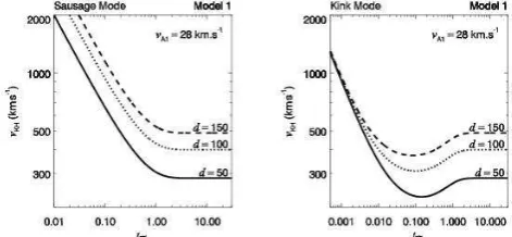
Fig. 1.Variation of the Kelvin-Helmholtz speed,vKH, with
the dimensionless quantity kz0 for model 1 on logarithmic
scale for three different values of the density contrast be-tween the solar prominence and surrounding solar corona.
150, respectively. For model 2, we assume that our setup describes the situation of a dark plume, where the internal Alfv´en speed is vA1 = 200 km s−1, that is surrounded by
the prominence with a density contrast ofd= 0.05, 0.1 and 0.5, respectively, resulting in Alfv´en speeds of 44, 63 and 141 km s−1, respectively.
A key parameter in our discussion is the productkz0,
where k is the wavenumber of the waves under study and z0 is the width of the slab. Since our analysis refers to two
possible scenarios (prominence slab surrounded by coro-nal plasma and prominence slab surrounded by prominence plasma), the value of this parameter (kz0) takes different
values. In the first case we are going to assume (hypotheti-cally) that the entire prominence can be considered as one single plasma slab, in which case we are going to consider that z0 is the width of the prominence. The typical width
of prominences varies between 4 and 30 Mm (Lin 2010), meaning that the productkz0 falls in the interval 0.01 and
30. For the second scenario, we are going to consider that z0 refers to the size of a thread only, that has a width of
100-600 km, meaning that the dimensionless parameterkz0
will be in the interval 0.001 and 0.6.
One key aspect to note is that regardless of the model employed, the KH speed is always super-Alfv´enic. Under prominence conditions, these speeds amounts to values that are of the order of a few hundred km s−1. This would also
mean that, in prominences, the plasma is always Kelvin-Helmholtz stable. The variation of the threshold speed at which waves propagating in the slab become KH unstable is shown, on logarithmic scale, in Fig. 1 for model 1 with the threshold increasing with the wavelengths for both sausage and kink modes. For both types of waves the range of speed obtained clearly show that the existence of flows larger than vKH are not possible to observe, meaning that the
promi-nence in this model is indeed KH stable. For large values of kz0(wide slab or long wavelength approximation) the value
of the Kelvin-Helmholtz speeds reaches the value obtained for a single interface (see, e.g. Ballai et al. 2015). It is also clear that the threshold were waves become KH unstable increases with the density contrast between the prominence and the solar corona.
In the case of model 2, the range of kz0 is
differ-ent and observations restrict us to the situation when the wavelength of waves is larger than the width of the slab (see Fig. 2). In the case of sausage waves, vKH shows a
at-Fig. 2.Same as Fig. 1, but for model 2
tained forkz0= tanh −1v
A1d/vA2and here the value of the
vKH =vA1+vA2. For kink waves the KH threshold shows a
1/kz0-type monotonic decrease. For small values of the
di-mensionless quantitykz0, the KH threshold for kink waves
is much larger than the corresponding value for sausage modes, while they tend to become equal for kz0≈1. This
result shows that, for long wavelengths, sausage waves can become much easily KH unstable than kink waves, how-ever, the range of speeds obtained here is inconsistent with the values observed for background flows.
Now using the definition ofωi together with the
disper-sion relations (17)–(18) we obtain that the imaginary part of the frequency in the first model is given by
ωi1=∓
k2
2Γ
4νtanhkz
0(dv0±Γ)
d+ tanhkz0 −
−ηCv 2
A1d(d+ tanhkz0)
v0tanhkz0∓Γ
, (22)
where the Cowling resistivity in the solar prominence is given by
ηC= 109Tp−3/2+
(2µ−1)v2 A1mp
2(1−µ)ρ1Σin πm
p kBTp
1/2
, (23)
whereTpis the temperature in the prominence. Here we
as-sumed that the plasma is made up of hydrogen and, there-fore, the mass of ions is equal to the mass of protons. We need to note here that a positive imaginary part of the fre-quency would mean that the amplitude of waves will grow despite the presence of dissipation, that is these waves are undergoing a dissipative instability.
For model 2, following the same technique, the imagi-nary part of the frequency becomes
ωi2≈ ∓
k2(d+ tanhkz 0)
2Γ
− ηC1v 2 A1d
v0tanhkz0∓Γ
+
+ηC2v
2
A2tanhkz0
dv0±Γ
. (24)
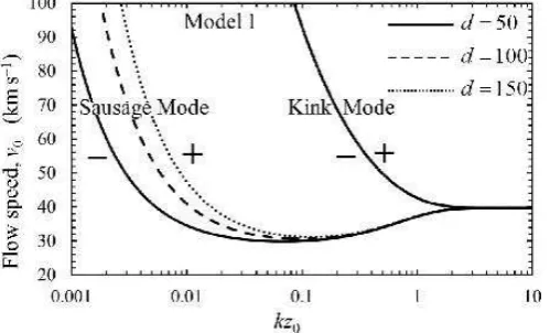
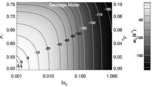
[image:7.595.55.293.58.177.2]Now let us investigate graphically the regions where the plasma becomes unstable, that is we search for the combi-nation of physical parameters that make the imaginary part of the frequency positive. As we specified earlier, the flows that are currently observed in solar prominences are of the order of a few tens of km s−1. In the case of model 1 we first plot the frequency contour plot of backward propagating waves (see Fig. 3) showing the regions where the imaginary
Fig. 3. Contour plot of the variation ofωi1 in the case of
sausage (left-hand side curves) and kink (right-hand side curves) modes in terms of background equilibrium flow and the value of the dimensionless parameter kz0 for model 1.
The ionisation rate isµ= 0.95.
part of the frequency is changing sign for a given value of the ionisation factor, µ= 0.95 (here and thereafter we are go-ing to concentrate mainly on backward propagatgo-ing waves as forward propagating waves will have a standard physical damping). The region above each curve corresponds to a combination of parameters that makes the imaginary part of the frequency positive, meaning that backward propa-gating waves are unstable. For values of equilibrium flows that are closer to observed values (the lower end of the flow interval considered here), it is possible to obtain two values ofkz0whereωi1is changing sign, that is the domain ofkz0
where waves are unstable is bounded by the two values. For example, for d= 50 and v0 = 35km s−1, ωi1 >0 for
0.009338< kz0<0.6246. The plots in Fig. 3 were obtained
for three different values of densities contrast and it is ob-vious that the threshold value for sausage modes depends on the value of density contrast only for larger values of flows. In the case of kink modes the three curves are in-distinguishable, so the instability threshold does not show any dependence on the density contrast. This behaviour could be explained in terms of the internal motion of the plasma in the two wave modes. In the case of kink waves, the slab oscillates without disturbing the internal structure of the slab, while, in the case of sausage modes, the inter-nal plasma structure is compressed and relaxed according to the oscillating pattern of the wave. While the instability of sausage modes sets in for smaller values of kz0 (in the
long wavelength limit), kink waves become unstable only when their wavelength is comparable with or shorter than the width of the slab.
Let us investigate how the instability threshold varies with the ionisation degree of the prominence slab. We choose a particular value of the equilibrium flow of 30 km s−1and letµvary between 0.5 and 1, corresponding to the
ionisation state of the plasma (see Fig. 4). We also fix three values of density contrast (d=50, 100, 150) between the prominence and solar corona. In the case of sausage modes, the threshold of instability depends on the ionisation degree for very limited interval ofkz0. For this particular value of
[image:7.595.311.561.60.211.2]sig-Fig. 4. Contour plot of the variation ofωi1 in the case of
sausage modes in terms of ionisation degree and the value of the dimensionless parameterkz0for model 1. Herev0= 30
km s−1. The region where instability occurs is shown by
theplussymbol.
nificant dependence on the ionisation degree occurs only near the end of the interval. Density differences between the two media also influence the instability threshold. Fig. 4 shows that, as the density contrast increases, the thresh-old moves towards the direction of increased ionisation. The corresponding plot for kink waves is not shown here, as the appearance of unstable modes involves very high values of the equilibrium flow, therefore the appearance of instability is unrealistic.
Let us now discuss the second model that we use to study the instability of waves propagating in prominence dark plumes. Observations by Berger et al. (2008, 2011) and Ryutova et al. (2010) revealed that dark plumes are turbu-lent upflows in prominences which usually develop Kelvin-Helmholtz vortex rolls. Ca II absorption lines in promi-nence plumes show these as dark features, in contrast to the prominence material, which suggests a hotter plasma in the plumes compared to their environment. Plumes are also less dense than their surrounding material. The width of plumes ranges between 0.5 Mm to 6 Mm and their max-imum heights are between 11 Mm and 17 Mm. The mean flow speed is about 15 km s−1, although velocities up to 30
km s−1 are also measured, while the typical plume lifetime
is between 400 s and 890 s (Berger et al. 2010).
In this model the plasma inside and outside the slab are partially ionised and the plasma inside the slab exhibits an equilibrium flow along the background magnetic field. These structures are hotter and less dense than their envi-ronment, therefore d < 1. We assume that the plasma in the plume is nearly completely ionised, therefore we choose µ1= 0.55. The ionisation degree of the prominence (region
2) is unknown. We letµ2vary in the interval 0.55-0.95. Let
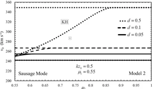
us first discuss the sausage modes appearing in these struc-tures. The parameter domains where the imaginary part of the frequency of backward propagating sausage modes changes sign are shown in Fig. 5. First to note is that the values of the equilibrium flow at which the backward mode is unstable for all three values of the density contrast are far too high. For flow spends that are observed modes are stable and they encounter a normal physical damping. Backward propagating waves become unstable for flow speeds that are comparable with the KH speeds. In Fig. 5, backward
propa-Fig. 5. Contour plot of the variation ofωi2 in the case of
sausage modes in terms of the equilibrium flow speed and the value of the dimensionless parameter kz0 for model 2.
The values of the density is shown in the legend of the figure. The region where instability occurs is shown by the
[image:8.595.313.561.57.208.2]plussymbol.
Fig. 6. Contour plot of the variation ofωi2 in the case of
sausage modes in terms of the equilibrium flow speed and the ionisation degree of the external region for model 2. The values of the dimensionless quantitykz0and the ionisation
degree of the plasma slab has been fixed and shown on the figure. The region where instability occurs is shown by the
plussymbol.
gating waves are unstable only in a narrow band shown by a
plussign. Above the upper boundary of the instability zone, the plasma becomes KH unstable. Similar findings can be obtained for other density contrasts. In Fig. 6, the appear-ance of the unstable regime of the same sausage mode is displayed for a fixed value ofkz0and we allow the variation
of the ionisation of the external medium to change between the extreme cases of a near complete ionisation and near neutral gas. Similar to the findings of Fig. 5, the values of flows at which the instability sets in is at around 250 km s−1, clearly for values higher than any measured flow
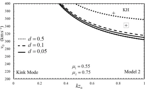
[image:8.595.43.291.58.211.2] [image:8.595.312.562.302.446.2]Fig. 7. Similar to Fig. 5, but here we plot the regions of instability for kink waves.
In the case of kink waves (see Fig. 7), the instability sets in, again, for very large values of the equilibrium flows and for very long wavelengths. The unstable region, again, is bounded, similarly to the domain shown in Fig. 4. Finally, for the same kind of waves, the instability threshold is prac-tically independent on the ionisation degree (for a fixed value ofkz0).
The very large values of equilibrium flows at which dissi-pative instabilities occur in filamentary structures lead us to the necessity of an alternative treatment of the partially ionised prominence plasma stability.
Two-fluid approximation
The above one fluid models are restricted to periods that are larger than the ion-neutral collisional time. For peri-ods that are less or comparable to the ion-neutral colli-sional time, the plasma dynamics is described in a two-fluid approximation, where the equations are written for the charged particles (ions and elections) and neutrals. The plasma behaviour of the mixture is ensured by collisional terms between ions and neutrals in the induction equa-tion and these collisional are dominant processes in mo-mentum transfer between species and the electron inertia is neglected. In reality, the two models are not identical, instead they are complementary.
Similarly to the equilibrium described earlier in this study (model 2), we are going to consider that the equilib-rium configuration is composed of a partially ionised slab filled with plasma in steady state (v0 is the equilibrium
flow and is parallel to the discontinuity), surrounded by two partially ionised half-space plasma regions. The plasma is permeated by a homogeneous magnetic field oriented in the x direction, and the interfaces are situated at z = 0 andz=z0. The equilibrium plasma parameters are
homo-geneous and constants in all regions. We denote the regions inside and outside the slab by the indices 1 and 2, respec-tively.
The set of coupled differential equations governing the dynamics of linear waves in incompressible two-fluid plas-mas is given by (see, e.g. Zaqarashvili et al. 2011, Khomenko et al. 2014a, Mart´ınez-G´omez et al. 2015 )
ρ0i
∂vi
∂t +v0· ∇vi
=−∇pie+ 1 µ0
(∇ ×b)×B0−
−αin(vi−vn), (25)
ρ0n
∂vn
∂t +v0· ∇vn
=−∇pn−αin(vn−vi), (26)
∂b
∂t =∇ ×(v0×b) +∇ ×(vi×B0) +R1, (27)
∇ ·vi=∇ ·vn=∇ ·b= 0, (28)
where vi= (vix,0, viz) andvn= (vnx,0, vnz) are the
com-ponents of the two-dimensional velocity perturbation of ions and neutrals,pieandpnare the pressure perturbations
of the ion-electron and neutral fluids, b= (bx,0, bz) is the
magnetic field perturbation,ρ0iandρ0nare the equilibrium
densities of ions and neutrals, while αin is the ion-neutral
friction coefficient. Frictions between charged and neutral (close-range interaction) particles is ensured via collision processes. In the absence of this process, neutrals will not be able to stay in the system and the momentum equa-tions would decouple. Equaequa-tions (25) and (26) are the lin-earized momentum equations of the ion-electron fluid and neutrals, respectively. The last terms on their RHSs ex-press the transfer of momentum between ions and neutrals through diffusion of one species into the other. As a result of collisions, particles can loose energy. The dynamics in the external region is described by a similar system of equa-tions, with the exception that the equilibrium outside the slab is static. As pointed out by Zaqarashvili et al. (2011), Cowling resistivity appears only in the one fluid approx-imation, that is why in Eq. (27) R1 = η∇2b, where the
coefficient of resistivity appears only due to the movement and interaction of electrons in the partially ionised plasma and is defined as
η= c
2(ν
ei+νen) ω2
pe ,
whereνeiandνenare the electron-ion and electron-neutrals
collisional frequencies and ωpe is the electron plasma
fre-quency. According to Braginskii (1965) and Zaqarashvili et al. (2011) the two collisional frequencies are defined as
νei=
√
12nee4ln Λ
12π3/2ǫ2 0m
1/2
e (kBT)3/2
, νen= Σennn 8k
BT πmn
1/2
,
whereneis the number density of electrons,eis the electron
charge, ln Λ is the plasma logarithm, ǫ0 is the permitivity
of free space and Σen = 10−19 m2 is the electron-neutral
collision cross-section. The electron plasma frequency is a quantity that depends only on the number density of elec-trons and is defined asωpe≈17.8πn1e/2 (s−1). Introducing
the values of physical constant and assuming ln Λ≈15 we arrive to the relation
η=
4.95(1
−µ)T1/2
2µ−1 +
15.81×10⁸
T3/2
(m2s−1),
where the temperature is measured in K. Equation (27) clearly shows that the magnetic field is able to interact only with the charged part of the plasma fluid.
Let us express the ion-neutral friction coefficient,αin,
as
whereγinis the ion-neutral collision rate coefficient per unit
mass. The friction coefficient vanishes in both the fully ion-ized (ρ0n = 0) and fully neutral (ρ0i = 0) cases. However,
instead of using γin, we are going to use the collision
fre-quency, which has a more practical physical meaning. Thus, we define the ion-neutral,νin, and neutral-ion,νni, collision
frequencies as
νin=ρ0iγin, νni=ρ0nγin, (30)
and the two collisional frequencies are connected through ρ0nνin =ρ0iνni. In consequence, in the remaining part of
the present paper, we are going to use νin only and use ν1 and ν2 to denote the collisional frequencies in the two
media.
We are going to employ the same normal mode analysis as in the case of single fluid description here, however, the continuity of the normal component of momentum across the discontinuity would require an equivalent relation writ-ten for ions and neutrals. Similarly, the continuity of the stresses at the interface would translate into the balance of the total pressure of charged particles and the kinetic pressure of neutrals.
After straightforward calculations we can obtain that the dispersion relation for waves propagating along the in-terface in the incompressible limit can be given as DR+ iDI = 0, where now the real and imaginary parts of the
dispersion relation are given by
DR= (DA1di+DA2tanhkz0)(Ω2dn+ω2tanhkz0),
DI = (DA1di+DA2tanhkz0)(Ων1dn+ων2tanhkz0)+
(Ω2dn+ω2tanhkz0) [Ωdiν1χ1+ων2χ2tanhkz0+
+k4 v2
A1η1di
Ω +
v2
A2η2tanhkz0
ω
. (31)
where DA1 = Ω2−k2vA21, DA2 = ω2 −k2vA22, χ1,2 =
ρ0n1,2/ρ0i1,2 and dn =ρ0n1/ρ0n2, di =ρ0i1/ρ0i2. The
dis-persion relation given by Eq. (31) describes the propaga-tion of two pairs of waves propagating in the opposite di-rection, in each direction having a wave that is connected to ions, while the other one to neutrals. The collisions be-tween species lead to the modification in the amplitude of waves. The presence of collisions between particles (and the associated momentum transfer) together with the resistiv-ity renders the equations to be dissipative. Due to the loss of energy and momentum of individual species waves will propagate with a complex frequency, where the imaginary part describes damping or amplification.
Despite lacking a firm physical basis from the partially ionised plasma point view, let us discuss the collisionless and ideal limit, that is when ν1 = ν2 = η1 = η2 = 0
(in the absence of collisions, neutrals cannot be kept in the system), as this will help us understand the results obtained in the collisional limit. In this case, the dispersion relation is decoupled and we can solve separate equations for ions and neutrals. Accordingly, the dispersion relation for ions becomes
DA1di+DA2tanhkz0= 0, (32)
which can be easily solved to lead to
ω=kv0di±
p
ditanhkz0(vKH2 −v02)
di+ tanhkz0
, (33)
where the Kelvin-Helmholtz speed is defined as
v2 KH=
(di+ tanhkz0)(vA21di+vA22tanhkz0)
ditanhkz0
.
As Eq. (33) shows, the ion wave becomes KH unstable for flow speeds larger than vKH. However, since vKH is
al-ways super-Alfv´enic in an incompressible plasma and the observed flows are always sub-Alfv´enic, waves due to ions will be always KH stable.
In the case of neutrals, the dispersion relation in the collisionless limit becomes
Ω2dn+ω2tanhkz0= 0, (34)
whose solution reads
ω=kv0dn±iv0
√
dntanhkz0
dn+ tanhkz0
. (35)
This dispersion relation describes the propagation of two waves in the same direction, however, one of them is damped, while the other is amplified in time. These modes owe their existence to the presence of the equilibrium flow, and the flow plays the role of reservoir/sink for gained/lost energy of the wave. The peculiar behaviour of neutrals un-der prominence conditions was discussed earlier (see, e.g. Soler et al. 2012) and the unstable behaviour corresponds to the standard hydrodynamic KH instability. Another impor-tant result of this limit is that a two-fluid approach allows the propagation of two pairs of waves, one due to charged particles, and the other one for neutrals. In contrast, a single-fluid approach allows the propagation of one single pair, and this mode is a surface Alfv´en wave. Similarly to the single-fluid approach, we are interested in the backward propagating waves that can develop dissipative instability. Let us first concentrate on the ion-related waves, for which the dispersion relation (in the uncoupled limit) of the backward propagating wave is given by Eq. (33), where we choose the lower sign. Using Cairn’s criteria, the imaginary part of the frequency is approximately given by Eq. (19) where the equation is evaluated at the roots of the ideal dispersion relation, that is the solutions obtained in the collisionless limit.
After straightforward calculations we obtain that the imaginary part of the frequency of the backward propagat-ing wave is given by
ωii≈ θ1+θ2
2˜Γ1(di+ tanhkz0)
, (36)
where
θ1=
k2(d
i+ tanhkz0)2
(v0di−˜Γ1)(˜Γ1+v0tanhkz0) h
˜
Γ1(vA21η1di+v2A2η2)+
+v0(vA22η2tanhkz0−vA21η1d2i)
θ2=−Γ˜1(diν1χ1+ν2χ2tanhkz0)−
v0tanhkz0di(ν1χ1−ν2χ2),
and ˜Γ1= p
ditanhkz0(v2KH−v02).
are ionised, therefore, dn < 1. The ion-neutral collisional
frequency depends on the temperature and densities of the plasma. Let us consider that ν1 = αν2. As a result, the
ratio of the collisional frequencies becomes
α= ν1 ν2
=ρ0n1 ρ0n2
r
T1
T2
=dn r
T1
T2
.
Although we restricted ourselves to the case dn < 1, the
fact that T1/T2 > 1 means that α can take any values.
As a representative collisional frequency between ions and neutrals in the prominence region we can estimate that the ion-neutral collisional time (for a hydrogen plasma) can be defined as
νin= 4nnΣin r
kBT πmi
. (37)
For typical prominence values (nn= 1016 m−3,T = 104 K
using the FAL3 model), we obtain a collisional frequency of the order of 208 s−1 (Fontenla et al. 1990, Oliver et al.
2016).
To bring theoretical results closer to observations, we express neutral densities in terms of ion densities, as current observations reveal number densities for ions, rather than neutrals. From Eqs. (1)-(3) we have
ρ0n1≈
ξn1ρ0i1
1−ξn1
,
and a similar relation is valid in region 2. It is easy to calculate the new expression ofdn as
dn=di
(2µ1−1)(1−µ2)
(1−µ1)(2µ2−1)
,
where µ1 and µ2 are the ionisation fractions inside and
outside the slab, respectively.
Let us now consider that medium 1 is a plume and re-gion 2 represents the surrounding prominence. Based on ob-servations by Berger et al. (2010), we assume that plumes, having a temperature of 105 K, are surrounded by
promi-nence plasma with temperature of 104 K. Since the exact
ionisation degree of the prominence plasma is not known, we assume for illustration that µ2 = 0.75 and let the
ion-isation degree of the plume vary between 0.5 and 0.75. Furthermore, we consider that the ion density in the promi-nence isρi02= 5×10⁻¹¹kg m−3and a density of the plume
is 10% of it, that is ρ0i1 = 0.1ρ0i2, di = 0.1. For all types
of waves, we adopted a flow speed of 10 km s−1. Since the
imaginary part of the frequency is negative for both waves (regardless the ionisation degree), the waves will undergo a physical damping (Figs. 8–9). Similar to the one fluid model, the instability will set in for much larger values of flow, values that are currently not observed, however the more ionised the plasma is, the easier is to have an unsta-ble sausage wave. From this perspective, kink modes are more stable than sausage modes.
[image:11.595.312.564.55.199.2]Now let us look at the waves associated to neutrals where both waves are forward propagating. Now, if unsta-ble behaviour appears, it could be attributed to a Kelvin-Helmholtz instability (similar to the findings by Mart´ınez-G´omez et al. 2015). Since the mode corresponding to the lower sign is always damped, we will concentrate on the wave that corresponds to the upper sign in Eq. (35). In the collisionless limit the amplitude of this wave grows in
Fig. 8. Variation of the imaginary part of the frequency for backward propagating sausage modes due to ions in the two-fluid approximation with the ionisation degree of the plasma and the wavelength of waves.
Fig. 9.The same as in Fig. 8, but here the dispersion curves denote the imaginary part of the frequency of kink modes.
time. We should mention here that the imaginary part of the frequency given by Eq. (35) does not refer to any physi-cal effect. This value is the solution of the collisionless limit and it will be used next to determine the real (physical) damping or growth rate of these waves. Following the same procedure as before, the imaginary part of the frequency is given by Eq. (A.1) and it is clear that it is not affected by resistivity.
However, the expression given by Eq. (A.1) is not the full answer to our problem, since this has to be consid-ered together with the value determined earlier in Eq. (35). Combining the two relations, we arrive at the imaginary part of the frequency that appears due to neutrals
ω+in=ω+in+
kv0√dntanhkz0
(dn+ tanhkz0)
. (38)
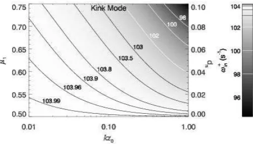
The variation of the imaginary part of the frequency (coun-terplots) is shown in Figs. (10)–(11), for sausage and kink modes, respectively. This result clearly shows what new physics is brought into these systems by neutrals. While kink waves are unstable for the whole range of parameters, the instability threshold for sausage modes depends on the ionisation degree of the plasma and the wavelength of waves (Fig. 10). In the long wavelength limit (kz0≪1) waves are
[image:11.595.314.563.261.403.2]Fig. 10. Variation of the imaginary part of the frequency for propagating sausage modes in the two-fluid approxima-tion.
Fig. 11. The same as in Fig. 10, but here the dispersion curves denote the imaginary part of the frequency of kink modes.
In addition, there will be a wavelength cut-off value (here corresponding to kz0 ≈ 0.03) after which modes will
be-come unstable, regardless the amount of neutrals in the system. In the case of sausage modes the growth rate of waves (for fixed wavelength) decreases with increasing the number of neutrals in the plume region. The same pattern is recovered for kink modes, however, the growth rate is weakly affected by the presence of more neutrals. Therefore, neutrals indeed have a stabilising effect on sausage modes due to the increased amount of the momentum transferred by neutrals in the process of collision. For a fixed ionisation degree, the frequency increases with decreasing wavelength, so that the longer the wavelength, the shorter is the growth time of sausage waves.
These results show that the consideration of a two fluid MHD for model 2 introduces a new physics that has not been possible to describe in the framework of a single fluid MHD. The two regimes are difficult to compare, as they are valid in different frequency regimes. It remains to be seen what the temporal evolution of these instabilities is (e.g. they can saturate, evolve into a macro instability, or develop turbulences), but this issue would require a robust numerical investigation. The mixture of two species plasma, therefore, shows a very complex pattern where the Kelvin-Helmholtz unstable behaviour of neutrals is stabilised by the damping due to collisions with ions. Since the species of the plasma are coupled through collisions, the instability
of one single species will drive the whole mixture into an unstable state.
Finally, we need to mention that our results are some-how quantitatively different from the results obtained ear-lier by Mart´ınez-G´omez et al. (2015), but this is due to the technique used here to find the imaginary part of the fre-quency. While the above authors used numerical methods to study the onset of the KHI in a two-fluid model, our analytical approach is valid only for weakly dissipative and low collisional frequency plasmas.
5. Conclusions
The present research focussed on the appearance of dissipa-tive instabilities for waves propagating in a partially ionised plasma slab surrounded by the corona or another partially ionised prominence environment. The geometrical restric-tions imposed on waves make them dispersive, and different characteristics were investigated for symmetric and asym-metric waves (sausage and kink waves).
The nature of the instabilities discussed here means that they appear for flow speeds lower than the KHI, the value of the KH speed playing a special role in our discussion. A simple analysis showed that the KHI is unlikely to occur in the plasmas we dealt with. The threshold values where the KH instability occurs varies with the density ratio of the slab plasma and its surrounding and with the wavelength of the waves. In all cases, the flow speed at which waves are KH unstable is of the order of a few thousand km s−1, that
is much above currently observed values.
We analysed the appearance of dissipative instability, that is the unstable growth of a backward propagating wave in the presence of flow, in two different equilibrium set-ups. First we assumed that the whole partially ionised promi-nence can be treated as a slab surrounded by the viscous and completely ionised corona. After imposing the neces-sary boundary conditions at the interfaces between the two media, we derived a dispersion relation describing the prop-agation of incompressible waves propagating inside the slab. The imaginary part of the frequency describes the damping or the growth of waves. The results on the role of viscosity and magnetic field are identical with the findings by Ballai et al. (2015). Here we focussed on the role of dispersion and the ionisation degree on the stability threshold of waves. Our results show that sausage modes are more sensitive to the variation of physical parameters, the value of ionisation degree is more pronounced for very large wavelengths.
The second model we used is a plasma slab in partially ionised state surrounded by another partially ionised, in-finitely extended environment, modelling the case of promi-nence dark plumes surrounded by another promipromi-nence ma-terial. Our results clearly show that the unstable behaviour of these structures require unrealistically high flows as long as the periods of waves are larger than the ion-collisional time and the plasma dynamics is described in a one-fluid MHD model. The situation is different when we consider very high frequency waves (or low periods) when the plasma behaviour requires a two-fluid approach.
[image:12.595.44.295.251.394.2]neutrals. The source of instability for this mode in a single-fluid MHD approach does not exist. Strictly speaking the instability described here is not dissipative in the sense of instabilities described earlier, as the modes that are unsta-ble are forward propagating.
Large values of flow necessary for an instability to oc-cur in a single fluid MHD model is not a surprise, given the simplicity of our model. We are aware that the simple model employed here misses several key effects for plume dynamics. For example, the sharp interface considered here does not allow the appearance of body waves, that could be important concerning the stability of plumes. Furthermore, the flow of particles oblique to the magnetic field might de-crease the instability threshold significantly, as it was shown by Prialnik et al. (1986) in the case of KH instability. It also remains to be seen how the effect of compressibility can change the stability criteria, bearing in mind that the general effect of compressibility is to stabilise the plasma.
Acknowledgements. The authors are grateful for the support by the Leverhulme Trust (IN-2014-016). R.O. acknowledges support from MINECO and FEDER funds through project AYA2014-54485-P. The authors would like to thank R. Soler, D. Mart´ınez-G´omez, and the anonymous referee for their suggestions
References
Arber, T.D., Botha, G.J.J., & Brady, C. S., 2009, ApJ, 705, 1183 Arber, T.D., Haynes, M., & Leake, J. E., 2007, ApJ, 666, 541 Ballai, I., Oliver, R., & Alexandrou, M. 2015, A&A, 577, 82 Berger, T.E., Shine, R.A., Slater, G.L. et al., 2008, ApJ, 676, 89 Berger, T.E., Slater, G.L., Hulburt, N. et al., 2010, ApJ, 716, 1288 Braginskii, S. I., 1965, Transport Processes in a Plasma, Reviews of
Plasma Physics, Vol. 1 (New York: Consultants Bureau) Carbonell, M., Forteza, P., Oliver, R., & Ballester, J.L. 2010, A&A,
515, 80
Cairns, M. 1979, J. Fluid Mech., 92, 1
Cowling, T.G., 1957, Magnetohydrodynamics, Monographs on Astronomical Subjects, Adam Hilger (Bristol)
Diaz, A.J., Khomenko, E., & Collados, M., 2014, A&A, 564, 97 Diaz, A.J., Soler, R. & Ballester, J.L., 2012, ApJ, 754, 41 Edwin, P.M., & Roberts, B. 1982, Sol. Phys., 76, 239
Fontenla, J.M., Avrett, E.H. ,& Loeser, R. 1990, ApJ, 335, 700 Forteza, P., Oliver, R., Ballester, J.L., & Khodachenko M.L., 2007,
A&A, 461, 731
Forteza, P., Oliver, R. & Ballester, J.L., 2008, A&A, 492, 223 Gilbert, H., Kilper, G., & Alexander, D., 2007, ApJ, 671, 978 Goodman, M.L. 2001, Space Sci. Rev., 95, 79
Hillier, A., Shibata, K., & Isobe, K., 2010,PASJ, 62, 1231
Hirayama, T., 1986 in Coronal and Prominence Plasmas, ed. Poland, A.I. (NASA Conf. Publ., Vol 2442, Whashington D.C.: NASA), 149
Joarder, P.S & Roberts, B., 1992, A&A, 256,625
Khodachenko, M. L., Arber, T.D, Rucker, H.O., & Hanslmeier, A., 2004, A&A, 422, 1073
Khomenko, E., Collados, M, Diaz, A., & Vitas, N., 2014a, Phys. Plasmas, 21, 092901
Khomenko, E., Diaz, A., de Vincente, A., Collados, M, & Luna, M., 2014b, A&A, 565, 45
Labrosse, N., Heinzel, P., Vial, J. et al., 2010, Space Sci. Rev., 151, 243
Leake, J.E., & Arber, T.D. 2006, A&A, 450, 805
Leake, J.E., Arber, T.D., & Khodachenko, M.L. 2005, A&A, 442, 1091 Liggett, M., & Zirin, H., 1984, Sol. Phys., 91, 259
Lin, Y., 2010, Space Sci. Rev., 158, 237
Lin, Y., Engvold, O., & Wiik, J.E., 2003, Sol. Phys., 216, 109 Mart´ınez-G´omez, D., Soler, R., & Terradas, J. 2015, A&A, 578, 104 Murawski, K., Chmielewski, P., Zaqarashvili, T.V., & Khomenko, E.,
2016, MNRAS, 459, 2566
Ni, L., Yang, Z., & Wag, H. 2007, Astrophys. Space Sci. 312, 139 Okamoto, T.J., Tsuneta, S., Berger, T.E. et al. 2007, Science, 318,
1577
Oliver, R., Soler, R., Terradas, J., & Zaqarashvili, T.V., 2016, ApJ, 818, 128
Patsourakos, S., & Vial, J.-C. 2002, Sol. Phys., 208, 253
Prialnik, D., Eviatar, A., & Ershkovich, A.I., 1986, J. Plasma Phys., 35, 209
Ruderman, M. S. 2015, A&A, 580, 37
Ryutova, M. P., Berger, T.E., Frank, Z., Tarbell, T., & Title, A. 2010, Sol. Phys., 267, 75
Shadmehri, M., Yaghoobi, A., & Khajavi, M. 2013, Astrophys. Space Sci., 347, 151
Singh, K.A.P. & Krishan, V., 2010, New Astron., 15, 119 Soler, R., Oliver, R., & Ballester, J.L., 2009, ApJ, 707, 662
Soler, R., Diaz, A. J., Ballester, J.L. ,& Goossens, M., 2012, ApJ, 749, 163
Zaqarashvili, T.V., Khodachenko, M.L., & Rucker, H.O., 2011, A&A, 529, 82
Appendix A: The imaginary part of the frequency
calculated for neutrals
The imaginary part of the frequency calculated with the help of Cairn’s formula (see Eq. (19) that corresponds to the positive (ampli-fied) solution of the collisionless dispersion relation attached to neu-trals is given by
ω+in=−
1 2(dn+ tanhkz0)
ν1dn−ν2tanhkz0+
Ψ+ 1
Ψ+2
, (A.1)
where
Ψ+1 = 2dntanh 2kz
0(ν1−ν2)
v2
0(di−dn)
(dn+ tanhkz0)2
,
Ψ+ 2 =
v2
0(di−dn) tanhkz0
(dn+ tanhkz0)2