Rotating quantum states

Contents lists available atScienceDirect

Physics Letters B

www.elsevier.com/locate/physletb

Rotating quantum states

Victor E. Ambru ¸s, Elizabeth Winstanley

∗

Consortium for Fundamental Physics, School of Mathematics and Statistics, University of Sheffield, Hicks Building, Hounsfield Road, Sheffield, S3 7RH, United Kingdom

a r t i c l e

i n f o

a b s t r a c t

Article history: Received 14 April 2014

Received in revised form 13 May 2014 Accepted 15 May 2014

Available online 20 May 2014 Editor: M. Cvetiˇc

We revisit the definition of rotating thermal states for scalar and fermion fields in unbounded Minkowski space–time. For scalar fields such states are ill-defined everywhere, but for fermion fields an appropri-ate definition of the vacuum gives thermal stappropri-ates regular inside the speed-of-light surface. For a massless fermion field, we derive analytic expressions for the thermal expectation values of the fermion current and stress–energy tensor. These expressions may provide qualitative insights into the behaviour of ther-mal rotating states on more complex space–time geometries.

©2014 The Authors. Published by Elsevier B.V. This is an open access article under the CC BY license (http://creativecommons.org/licenses/by/3.0/). Funded by SCOAP3_.

1. Introduction

In the canonical quantisation of a free field, an object of fun-damental importance is the vacuum state, from which states con-taining particles are constructed. For fields of all spins, the process starts by expanding the classical field in terms of an orthonor-mal basis of field modes, which are split into positive and neg-ative frequency modes. The expansion coefficients are promoted to operators, the expansion coefficients of the positive frequency modes being particle annihilation operators.1 _{The vacuum state is} defined as the state annihilated by all the particle annihilation op-erators. The definition of a vacuum state is therefore dependent on how the field modes are split into positive and negative frequency modes. This split is restricted for a quantum scalar field by the fact that positive frequency modes must have positive Klein–Gordon norm. For a quantum fermion field, both positive and negative fre-quency fermion modes have positive Dirac norm, so the split of the field modes into positive and negative frequency is less constrained compared with the scalar field case. There is therefore more free-dom in how the vacuum state is defined for a fermion field, lead-ing to more freedom in how states containlead-ing particles are defined. In this letter we explore this difference between scalar and fermion quantum fields by considering the definition of rotating

*

Corresponding author.

E-mail addresses:app10vea@sheffield.ac.uk(V.E. Ambru ¸s),

e.winstanley@sheffield.ac.uk(E. Winstanley).

1 _{The adjoints of the expansion coefficients of the negative frequency modes are} also particle annihilation operators. For a real scalar field, these annihilation opera-tors are the same as the expansion coefficients of the positive frequency modes; for a fermion field they are different.

vacuum and thermal states in Minkowski space. This toy model reveals that there are quantum states which can be defined for a fermion field but which have no analogue for scalar fields.

2. Rotating scalars

We consider Minkowski space in cylindrical coordinates

(

tMink

,

ρ

,

ϕ

Mink

,

z

)

.2 We wish to define quantum states which are rigidly rotating with angular velocity

. Choosing thezaxis of the coordi-nate system along the angular velocity vector

, the line element of the rotating space–time can be found by making the transfor-mation

ϕ

=

ϕ

Mink

−

Ω

tMink,t

=

tMinkin the usual Minkowski line element, giving:

ds2

= −

1

−

ρ

2

Ω

2

dt2

+

2

ρ

2

Ω

dt d

ϕ

+

d

ρ

2

+

ρ

2d

ϕ

2

+

dz2

.

(1)

The Killing vector

∂

t, which defines the co-rotating Hamiltonian

H

=

i

∂

t, becomes null on the speed-of-light surface (SOL), defined as the surface where

ρ

=

Ω

−1. The Klein–Gordon equation for a scalar field of mass

μ

on the space–time(1)is:

−

(

H

+

Ω

Lz

)

2

+

L2_z

ρ

2

+

P

2 z

−

∂

ρ2

−

∂

ρ

ρ

+

μ

2

Φ(

x

)

=

0, (2)

where Pz

= −

i

∂

z andLz

= −

i

∂

ϕ are thezcomponents of the

mo-mentum and angular momo-mentum operators, respectively. The mode solutions of(2)are:

2 _{Throughout this paper we use units in whichc= ¯h=k}

B=1.

http://dx.doi.org/10.1016/j.physletb.2014.05.031

f_ωkm

(

x

)

=

1

8

π

2

_|

_ω

_|

e

−iωt+imϕ+ikz_J

m

(

q

ρ

),

(3)

where Jm

(

qρ

)

is the Bessel function of the first kind of orderm,

m is the eigenvalue of Lz,k is the eigenvalue of Pz,q is the lon-gitudinal component of the momentum and

ω

= ±

μ

2

₊

_q2

₊

_k2 gives the Minkowski energy of the mode. The eigenvalue of the Hamiltonian,

ω

=

ω

−

Ω

m, represents the energy of the mode as seen by a co-rotating observer. It is convenient to introduce the shorthand j

=

(

ω

j

,

kj

,

mj

)

and

δ

j

,

j

=

δ

mjmj

δ(

kj

−

kj

)

δ(

ω

j

−

ω

j

)

|

ω

j

|

.

(4)

Using the Klein–Gordon inner product:

f

,

g

= −

i

d3x

√

−

g

f∗

∂

tg

−

g

∂

tf∗

,

(5)

the norm of the modes(3)can be calculated:

fj

,

fj

=

ω

j

|

ω

j

|

δ

j

,

j

.

(6)

As discussed by Letaw and Pfautsch [1], particles must be de-scribed by modes with positive norm (

ω

j

>

0), implying the fol-lowing expansion for the scalar field operator:

Φ(

x

)

=

∞

mj=−∞

∞

μ

ω

jd

ω

j

pj

−pj

dkj

fj

(

x

)

aj

+

f∗j

(

x

)

a †

j

,

(7)

where pj

=

q2

j

+

k2j is the Minkowski momentum. The one-particle annihilation and creation operators, aj and a†j, satisfy

the canonical commutation relations

[

aj

,

a†_j

] =

δ(

j

,

j

)

. The

in-duced vacuum state

|

0

, satisfying aj

|

0

=

0, coincides with the Minkowski vacuum[1].

At finite inverse temperature

β

=

T−1, Vilenkin [2] gives the following thermal expectation value (t.e.v.):

a†_jaj

β

=

δ(

j

,

j

)

eβωj

−

₁

.

(8)

The above expression cannot hold when

ω

j

<

0[2], since it would imply that the vacuum expectation value ofa†_jaj, obtained by tak-ing the limit

β

→ ∞

, is non-zero, contradicting the definition of the vacuum. Furthermore, the divergent behaviour of the thermal weight factor of modes with

ω

close to 0 renders t.e.v.s infinite, causing rotating thermal states for scalar fields to be ill-defined everywhere in the space–time[2,3]. As discussed by[2,3], a resolu-tion to these problems is to enclose the system inside a boundary located inside or on the SOL, restricting wavelengths such that

ω

stays positive for all values ofm.

3. Rotating fermions

In the Cartesian gauge[4], a natural frame for the metric(1)

can be chosen to be:

e_ˆt

=

∂

t

−

Ω∂

ϕ

,

eˆi

=

∂

i

.

(9)

In the following, hats shall be used to indicate tensor components with respect to the tetrad, i.e. Aμ

=

Aαˆeμ_αˆ. The Dirac equation for fermions of mass

μ

takes the form:

γ

ˆt

(

H

+

Ω

Mz

)

−

γ

·

P

−

μ

ψ (

x

)

=

0, (10)

where the gamma matrices are in the Dirac representation[5]and the covariant derivatives are given by:

i D_ˆt

=

H

+

Ω

Mz

,

−

i Dˆj

=

Pj

.

(11)

The momentum operatorsPjand angular momentum operatorMz are:

Pj

= −

i

∂

j

,

Mz

= −

i

∂

ϕ

+

1 2

σ

3 0

0

σ

3

.

(12)

The Dirac equation(10)admits the following solutions:

Uλ_Ekm

(

x

)

=

√

1 8

π

2e

−iEt+ikz

⎛

⎝

1

+

μ_E

φ

λ_Ekm

2λE

|E|

1

−

μ_E

φ

λ_Ekm

⎞

⎠

,

(13)

where the two-spinor

φ

λ

Ekmis defined as:

φ

λ_Ekm

(

ρ

,

ϕ

)

=

√

1 2

⎛

⎝

1

+

2λ_pkeimϕJm

(

q

ρ

)

2i

λ

1

−

2λ_pkei(m+1)ϕ_J

m+1

(

q

ρ

)

⎞

⎠

,

(14)

where

λ

is the helicity [4,5], p

=

q2

₊

_k2 _{is the magnitude of} the momentum and E

= ±

p2

₊

_μ

2 _{controls the sign of the} Minkowski energy of the mode. The eigenvalues of the Hamilto-nian are

E

=

E

−

Ω(

m

+

1₂

)

, representing, as in the scalar case, the energy seen by a co-rotating observer. The notations j

=

(

Ej

,

kj

,

mj

, λ

j

)

and

δ

j

,

j

=

δ

λjλj

δ

mjmj

δ(

kj

−

kj

)

δ(

Ej

−

Ej

)

|

Ej

|

(15)

are useful to refer to modes and their norms. The latter can be computed using the Dirac inner product:

ψ,

χ

=

d3x

√

−

g

ψ

†

(

x

)

χ

(

x

).

(16)

It can be shown that

Uj

,

Uj

=

δ(

j

,

j

)

for all possible labels j

,

j. After choosing a suitable definition for particle modes (i.e. a range for the labels in j), the anti-particle modes can be constructed us-ing charge conjugation[4,5]:Vj

=

iγ2ˆU∗_j. Hence,Vj automatically inherits the same normalisation asUj, namely:

Vj

,

Vj

=

δ(

j

,

j

)

. Therefore there is no restriction on how the split into particle and anti-particle modes is performed, as long as the charge conjuga-tion symmetry is preserved.

According to Vilenkin [2], the definition of particles for co-rotating observers should be the same as for inertial Minkowski observers, with the field operator written as:

ψ

V

(

x

)

=

λj=±12

∞

mj=−∞

∞

μ

EjdEj pj

−pj

dkj

×

Uj

(

x

)

bj;V

+

Vj

(

x

)

d†_j;V

.

(17)

Vilenkin’s quantisation is equivalent to the one suggested by Letaw and Pfautsch[1]for the scalar field, yielding a vacuum state equiv-alent to the Minkowski vacuum. In contrast, Iyer [6]argues that the modes which represent particles for a co-rotating observer have positive frequency with respect to the co-rotating Hamilto-nian, implying the following expression for the field operator:

ψ

I

(

x

)

=

λj=±12

∞

mj=−∞

∞

Ej>0,|Ej|>μ

EjdEj pj

−pj

dkj

×

Ujbj;I

+

Vj

(

x

)

d†j;I

,

(18)

quan-tisation methods lead to the canonical anti-commutation relations

{

bj

,

b†_j

} = {

dj

,

d†_j

} =

δ(

j

,

j

)

. The ensuing quantum field theory

dif-fers in the two pictures, as the vacuum state corresponding to Iyer’s quantisation differs from the Minkowski vacuum. This can be seen by looking at the connection between the Iyer and Vilenkin one-particle operators:

bj;I

=

bj;V Ejis positive,

i2m+1d†_j;V Ejis negative,

(19)

and similarly fordj;I, where

j

=

(

−

Ej

,

−

kj

,

−

mj

−

1

, λ

j

)

. Thus, the Vilenkin vacuum state (i.e. the non-rotating Minkowski vacuum) contains particles as defined according to Iyer’s quantisation. Sim-ilarly, the Iyer vacuum contains particles as defined according to Vilenkin’s quantisation (i.e. relative to the Minkowski vacuum).

Vilenkin [2]also considered rotating thermal states for fermi-ons. In analogy with(8), he gives the following t.e.v.s relative to the Minkowski vacuum[2]:

b†_jbj

β

=

d†_jdj

β

=

δ(

j

,

j

)

eβEj

+

₁

.

(20) As in the scalar case,(20)is not valid when

Ej

<

0 [2]. However, in contrast to the scalar case, the modes with negative

Ej can be eliminated from the set of particle modes by using Iyer’s quan-tisation, without enclosing the system within a boundary inside the SOL. Furthermore, unlike the thermal factor for scalars(8), the Fermi–Dirac density of states factor(20)is regular for all

Ej.

Eq. (20) can be used to construct the t.e.v.s of the neutrino charge current operator and of the SET:

Jαˆ

(

x

)

=

1 2

ψ,

γ

αˆ1

+

γ

ˆ

5

2

ψ

,

(21a)

T_αˆσˆ

(

x

)

= −

i 4

[

ψ ,

γ

(αˆDσˆ)

ψ

] − [

D(αˆ

ψ

γ

σˆ)

, ψ

]

.

(21b)

Using the Vilenkin quantisation, we find the following t.e.v.s rela-tive to the Minkowski vacuum:

:[

ψ ψ

]

V

:

β

= −

μ

S+000

,

(22a)

:

Jˆz_V

:

_β

= −

1₂S−₁₀₀

,

(22b)

:

T_V;ˆtˆt

:β

=

S+₂₀₀

,

(22c)

:

TV; ˆρρˆ

:β

=

S+020

−

ρ

− 1_S×

011

,

(22d)

:

TV; ˆϕϕˆ

:β

=

ρ

−1S×011

,

(22e)

:

T_V;ˆzzˆ

:β

=

S+₂₀₀

−

S+₀₂₀

−

μ

2S+₀₀₀

,

(22f)

:

T_V;ˆtϕˆ

:β

=

1₄

ρ

−1S−₁₀₀

−

1₂

ρ

−1S+₁₀₁

−

1₂S×₁₁₀

,

(22g)

where the fermion condensate

:[

ψψ

]

V

:

β vanishes when

μ

=

0. The functions S±_abc andS×_abcintroduced above are defined as:

S∗_abc

=

1

π

2 ∞ m=−∞ ∞

μ dE

1

+

eβE p

0

dk Eaqb

m

+

1₂

c

J_m∗

(

q

ρ

),

(23)

where

∗ ∈ {+

,

−

,

×}

and the functions J_m∗ are given by:

J±_m

(

z

)

≡

J2_m

(

z

)

±

J_m2₊₁

(

z

),

J×_m

(

z

)

=

2Jm

(

z

)

Jm+1

(

z

).

(24)

Except when

μ

=

0, numerical integration must be used to cal-culate S∗_abc for arbitrary values of the mass. For massless fermions, the method outlined inAppendix A can be followed to obtain the following exact results (

ε

=

1

−

ρ

2

_Ω

2_):

1

μ

:[

ψ ψ

]

V

:

β

= −

1 6β2

_ε

−

Ω

2 8

π

2

_ε

2

2 3

+

ε

3

,

(25a)

:

J_Vz

:

β

= −

Ω

12β2

_ε

2

−

Ω

3

48

π

2

_ε

3

(4

−

3

ε

).

(25b)

To evaluate the massless limit of the t.e.v. of the fermion con-densate

:[

ψψ

]

V

:

β, the latter was divided by the mass factor in

Eq.(22a). In the above, the hat has been dropped from the index

of Jz _{to indicate that the result is with respect to the coordinate} basis. For the z component, this coincides with the tetrad compo-nent. The t.e.v. of the SET with respect to the coordinate basis has the following components:

:

TV;tt

:β

=

7

π

2

60β4

_ε

+

Ω

2 8β2

_ε

2

4 3

−

1 3

ε

+

Ω

4 64

π

2

_ε

3

8 9

+

56 45

ε

−

17 15

ε

2

,

(25c)

:

TV;ρρ

:β

=

7

π

2

180β4

_ε

2

+

Ω

2 24β2

_ε

3

4 3

−

1 3

ε

+

Ω

4 192

π

2

_ε

4

8

−

88 15

ε

−

17 15

ε

2

,

(25d) 1

ρ

:

TV;ϕt

:β

= −

ρ

Ω

7

π

2

60β4

_ε

2

+

13Ω2 72β2

_ε

3

16 13

−

3 13

ε

+

119Ω4 960

π

2

_ε

4

200 119

−

64 119

ε

−

1 7

ε

2

,

(25e) 1

ρ

2

:

TV;ϕϕ

:β

=

7

π

2

180β4

_ε

3

(4

−

3

ε

)

+

Ω

2 24β2

_ε

4

8

−

8

ε

+

ε

2

+

Ω

4

192

π

2

_ε

5

64

−

456 5

ε

+

124 5

ε

2

₊

17

5

ε

3

,

(25f)

and

:

TV;zz

:

β

= :

TV;ρρ

:

β for any value of the mass

μ

. The con-nection between the tetrad and coordinate basis components is made through:

Ttt

=

Tˆtˆt

+

2

ρ

Ω

Ttˆϕˆ

+

ρ

2

Ω

2Tϕˆϕˆ

,

(26a)

Ttϕ

=

ρ

Tˆtϕˆ

+

ρ

2

Ω

Tϕˆϕˆ

,

(26b)

Tϕϕ

=

ρ

2Tϕˆϕˆ

.

(26c)

The analytic results for

:[

ψψ

]

V

:

β,

:

JVzˆ

:

β and

:

TV;tt

:

βgiven by Eqs. (25) reveal a number of physical features. Firstly, they all contain contributions which are independent of the tempera-ture (equivalently, independent of

β

). These terms are unphysical as the t.e.v.s should vanish when the temperature is set to zero (

β

→ ∞

). These temperature-independent terms are generated by modes with

E

<

0 and arise because the Vilenkin quantisation

[2] has been used. If the Iyer quantisation [6] is employed, ana-lytic expressions for the corresponding t.e.v.s for massless fermions

:[

ψψ

]

I

:

β,

:

JIz

:

β and

:

TI;ασ

:

β are found from(25)by subtract-ing the temperature-independent parts, for example,

:

Jz_I

:

_β

= −

Ω

12β2

_ε

2

.

(27)

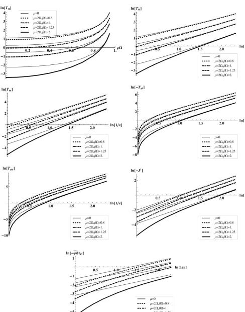
[image:4.612.60.548.77.697.2]

Fig. 1.Plots of the t.e.v.s in Eqs.(22)using Iyer’s quantisation for fermions with massμ=0 (thin lines) andμ=2Ω, at inverse temperatures (from top to bottom) 0.8, 1.0, 1.25 and 2.0, in units ofΩ−1_{. (a):T}

temperature-independent contributions to Eqs. (25) are absent from the t.e.v.s calculated using the Iyer quantisation.

If

Ω

=

0, there is no rotation and the t.e.v.s(25)reduce to the usual Minkowski t.e.v.s. If

Ω

=

0, on the axis of rotation we have

ε

=

1 and the expressions in round brackets in(25) evaluate to unity. In this case the t.e.v.s take the form of the Minkowski val-ues plus an

Ω

-dependent correction. A similar effect is found for rotating thermal states for a scalar field inside a reflecting cylin-der[3].

The t.e.v.s (25) are finite as long as

ε

>

0 but diverge as

ε

→

0 and the SOL is approached. Using the Iyer quantisation (when the

β

-independent terms are absent), the fermion conden-sate

:[

ψψ

]

I

:

βdiverges as

ε

−1, the current

:

JzI

:

βdiverges as

ε

−2 and the SET components

:

TIασ

:

β diverge as

ε

−4.

For the case of arbitrary mass, numerical methods can be em-ployed. In Fig. 1 we show the t.e.v.s in Eqs. (22) using the Iyer quantisation for massive fermions. As expected, increasing the mass damps the t.e.v.s. The damping becomes more pronounced as the temperature is decreased (

β

is increased). It can be seen from the log–log plots that as the SOL is approached, the t.e.v.s in the massive case diverge at exactly the same rate as for massless fermions. The mass contributes corrections which diverge at sub-leading orders, so that, close to the SOL, the quanta behave as if they were massless.

4. Conclusions

We have studied the construction of rotating states for scalar and fermion fields in four-dimensional Minkowski space. Our anal-ysis has demonstrated that the definition of fermion quantum states is less constrained than for scalar fields. This is due to more freedom in how the split into particle and anti-particle modes is performed for fermion fields, since all fermion modes have positive norm (the Dirac norm is positive definite but the Klein– Gordon norm is not). We have considered two possible quanti-sation schemes [2,6] for rotating fermion states, which yield two inequivalent vacuum states. We have computed thermal expecta-tion values (t.e.v.s) for rotating states relative to these two vacua. In the Vilenkin scheme[2], the vacuum state is equivalent to the (non-rotating) Minkowski vacuum, and t.e.v.s for rotating states relative to this vacuum include temperature-independent terms which arise from low energy modes having positive frequency as seen by a non-rotating observer but negative frequency as seen by a rotating observer. As discussed by Vilenkin[2], these low en-ergy modes (and hence the temperature-independent terms in the t.e.v.s) can be removed by enclosing the system within a boundary inside the speed-of-light surface.3 Using the Iyer scheme [6], the temperature-independent terms in the t.e.v.s are absent, without enclosing the system in a boundary or otherwise modifying the particle spectrum. As discussed in[6], we emphasize that the Iyer vacuum state cannot be defined for a quantum scalar field (which is restricted to the Minkowski vacuum). In addition, while rotating thermal states for scalar fields are ill-defined everywhere on the unbounded space–time[3], we have constructed fermion rotating thermal states which are regular inside the speed-of-light surface.

In this paper we have considered the toy model of rotating states in Minkowski space–time. However, the main physical fea-tures extend to curved space–times. For example, recent work on the construction of quantum states for fermion fields on a rotating Kerr black hole[8]has also demonstrated the existence of fermion states which have no analogue for scalar fields. Furthermore, the

3 _{Enclosing relativistic fermions within a boundary presents some difficulties[2].} We will return to this issue in a future publication[7].

simplicity of our toy model has enabled us to derive analytic ex-pressions for the thermal expectation values for massless fermions, which could provide qualitative insights into the behaviour of ther-mal rotating states on more complex space–time geometries, for example, the nature of the divergence as the speed-of-light sur-face is approached.

Acknowledgements

This work is supported by the Lancaster-Manchester-Shef-field Consortium for Fundamental Physics under STFC grant ST/ J000418/1, the School of Mathematics and Statistics at the Uni-versity of Sheffield and the European Cooperation in Science and Technology (COST) action MP0905 “Black Holes in a Violent Uni-verse”.

Appendix A. Fermi–Dirac integrals for massless rotating states

To compute the functions S∗_abc, defined in Eq. (23), the Fermi– Dirac density of states factor can be expanded about

Ω

=

0:

1

1

+

eβ[E−Ω(m+12)]

=

∞

n=0

(

−

Ω)

n

n

!

m

+

1₂

n

d

n

dEn

1 1

+

eβE

,

(A.1)

leading to:

S_abc∗

=

1

π

2

∞

n=0

(

−

Ω)

n

n

!

∞

μ

dE Ea d

n

dEn

1

eβE

₊

₁

×

p

0

dk qb

∞

m=−∞

m

+

1₂

n

+c

J∗_m

(

q

ρ

).

(A.2)

Sum over m

The sum overm in Eq.(A.2)vanishes unlessn

+

c is even for

∗ = +

and odd for

∗ ∈ {−

,

×}

. To perform the sum, the following formula can be used to rewrite the product of two Bessel functions as an infinite sum:

Jν

(

z

)

Jμ

(

z

)

=

∞

k=0

(

−

1)k

k

!

Γ (

ν

+

k

+

1)Γ (

μ

+

k

+

1)

×

Γ (

ν

+

μ

+

2k

+

1)

Γ (

ν

+

μ

+

k

+

1)

z

2

2k

+ν+μ

.

(A.3)

After the sum over m is performed, the above series terminates after a finite number of terms, as follows:

∞

m=−∞

m

+

1₂

2n

J_m+

(

z

)

=

n

j=0

2Γ (j

+

1₂

)

j

!

√

π

s +

n,jz

2j

_,

_(A.4a)

∞

m=−∞

m

+

1₂

2n

+1J_m−

(

z

)

=

n

j=0

2Γ (j

+

1₂

)

j

!

√

π

s −

n,jz

2j

_,

_(A.4b)

∞

m=−∞

m

+

1₂

2n

+1J_m×

(

z

)

=

n

j=0

2Γ (j

+

1₂

)

j

!

√

π

s ×

n,jz

2j+1

_,

_(A.4c)

wheres+_n,j can be shown to equal:

s+_n,j

=

1

(2

j

+

1)

!

αlim→0

d2n+1 d

α

2n+1

2 sinhα₂

2j

+1

.

(A.5)

d dz

z J_m+

(

z

)

=

(2

m

+

1)J−_m

(

z

),

d dz

z J_m×

(

z

)

=

2z J_m−

(

z

),

(A.6)

it can be shown thats−_n,jands_n×_,jare related tos+_n,j through:

s_n−_,j

=

j

+

1₂

s_n+_,j

,

s×_n,j

=

j

+

1 2

j

+

1s

+

n,j

.

(A.7)

Hence,s∗_n,j

=

0 for j

>

n. The following values ofs+_n,jare important for the calculation of the t.e.v.s in Eqs.(22):

s+_j,j

=

1, (A.8)

s+_j+1,j

=

1

24

(2

j

+

1)(2j

+

2)(2j

+

3), (A.9)

s+_j+2,j

=

1

5760

(2

j

+

1)(2j

+

2)(2j

+

3)(2j

+

4)

×

(2

j

+

5)(10j

+

3). (A.10)

The integral with respect to k

Following the steps in the previous paragraph, the sum overm involving the Bessel functions in J∗_m is replaced by a sum over j involving powers ofq. The integral overkcan be computed using:

p

0

dk qν

=

Γ (

ν

2

+

1)

√

π

2Γ (ν+₂1

+

1)p

ν+1

_.

_(A.11)

Analytic expressions in the massless case

Although the calculation of each individual function S∗_abc in Eqs.(22)has its own peculiarities, the method is very much the same. To illustrate the method, the simplest case a

=

b

=

c

=

0 shall be considered for the remainder of this section.

After performing the above steps, S+₀₀₀ can be brought to the following form:

S+₀₀₀

=

1

π

2

∞

j=0

(

ρ

Ω)

2j

j

+

1₂

∞

n=0

Ω

2ns+_n+j,j

(2

n

+

2j

)

!

×

∞

μ

dE p2j+1 d

2n+2j

dE2n+2j

1 1

+

eβE

.

(A.12)

In the above, the sums over j and n have been swapped, after which the sum over n was shifted down, i.e.

∞_n=0

n_j=0fn,j

→

_∞

j=0

_∞

n=0fn+j,j. While we do not have a method to compute the integral overE in Eq.(A.12)for arbitrary values of the mass

μ

, in the massless case, p

=

E and the integration can be done by parts:

∞

0

dE E2j+1 d

2n+2j

dE2n+2j

1 1

+

eβE

=

(2

j

+

1)

!

⎧

⎪

⎨

⎪

⎩

π2

12β2 n

=

0, 1

2 n

=

1,

0 n

>

1.

(A.13)

Then S+₀₀₀takes the form:

S+₀₀₀

=

∞

j=0

(

ρ

Ω)

2j

1 6β2

+

Ω

2

24

π

2

(2

j

+

3)

.

(A.14)

The sum over jcan be evaluated as a geometric series, giving:

S+₀₀₀

=

1

6β2

_ε

+

Ω

2 8

π

2

_ε

2

2 3

+

ε

3

,

(A.15)

where

ε

=

1

−

ρ

2

_Ω

2_.

The above algorithm can be applied to all other terms required for Eqs. (22). For brevity, the individual results shall not be in-cluded here, since the terms S∗_abc can be inferred from the final results(25), together with the relation

S×₁₁₀

=

1

ρ

S

+

101

−

1 2

ρ

d d

ρ

ρ

S−₁₀₀

.

(A.16)

References

[1]J.R. Letaw, J.D. Pfautsch, Phys. Rev. D 22 (1980) 1345.

[2]A. Vilenkin, Phys. Rev. D 21 (1980) 2260.

[3]G. Duffy, A.C. Ottewill, Phys. Rev. D 67 (2003) 044002.

[4]I.I. Cotaescu, J. Phys. A 33 (2000) 9177.

[5]C. Itzykson, J.B. Zuber, Quantum Field Theory, Dover Publications, 1980.

[6]B.R. Iyer, Phys. Rev. D 26 (1982) 1900.

[7] V.E. Ambru ¸s, E. Winstanley, in preparation.