Train unit scheduling with bi-level capacity requirements

This is a repository copy of

Train unit scheduling with bi-level capacity requirements

.

White Rose Research Online URL for this paper:

http://eprints.whiterose.ac.uk/102481/

Version: Accepted Version

Proceedings Paper:

Lin, Z, Barrena, E and Kwan, RSK (2015) Train unit scheduling with bi-level capacity

requirements. In: Proceedings. Conference on Advanced Systems in Public Transport

(CASPT 2015), 19-23 Jul 2015, Rotterdam, Netherlands. CASPT .

[email protected] https://eprints.whiterose.ac.uk/

Reuse

Unless indicated otherwise, fulltext items are protected by copyright with all rights reserved. The copyright exception in section 29 of the Copyright, Designs and Patents Act 1988 allows the making of a single copy solely for the purpose of non-commercial research or private study within the limits of fair dealing. The publisher or other rights-holder may allow further reproduction and re-use of this version - refer to the White Rose Research Online record for this item. Where records identify the publisher as the copyright holder, users can verify any specific terms of use on the publisher’s website.

Takedown

If you consider content in White Rose Research Online to be in breach of UK law, please notify us by

CASPT 2015

Train unit scheduling with bi-level capacity requirements

Zhiyuan Lin _· Eva Barrena _· Raymond S. K. Kwan

Abstract Train unit scheduling concerns the assignment of train unit vehi-cles to cover all the journeys in a fixed timetable allowing the possibility of coupling and decoupling to achieve optimal utilization while satisfying pas-senger demands. While the scheduling methods usually assume unique and well-defined train capacity requirements, in practice most UK train opera-tors consider different levels of capacity provisions. Those capacity provisions are normally influenced by information such as passenger count surveys, his-toric provisions and absolute minimums required by the authorities. In this paper, we study the problem of train unit scheduling with bi-level capacity requirements and propose a new integer multicommodity flow model based on previous researches. Computational experiments on real-world data show the effectiveness of our proposed methodology.

Keywords Train unit scheduling·Required train capacities· Multicommod-ity network flow

1 Introduction

A train unit is a self-propelled fixed set of rolling stock carriages (or cars)

that can move in either track directions on its own, in contrast to a tradi-tional combination of locomotive(s) and cars with the locomotive as the only power source. It is the most commonly used passenger rolling stock in the UK and many other European countries. A timetable is a set of train services

(conventionally called trains in the UK) during the operational period (one

working day) being planned, each of which has attributes mainly consisting of departure and arrival stations and times, seat demand, coupling and de-coupling possibilities, allowed types of train unit. Given a fixed timetable on

Z. Lin, E. Barrena, R. S. K. Kwan

School of Computing, University of Leeds, Leeds, LS2 9JT, United Kingdom Tel.: +44 (0)113 343 5430, Fax: +44 (0)113 343 5468

one operational day and a fleet of train units of multiple types, the train unit scheduling problem (TUSP) (Lin and Kwan (2013, 2014)) aims at deriving an optimized plan such that all the trains are covered with the required seat capacity provisions. From the perspective of a train unit, the problem assigns a sequence of trains to it as its daily workload. A notable feature of the TUSP is the activity of unit coupling/decoupling in response to different passenger demands. Generally, a train with a high demand requires more coupled units. In addition, coupling can also be used as a way of redistributing unit resources across the rail network regardless of the demand en route. Similar or relevant problems with respect to the TUSP include train unit circulation (Schrijver (1993); Alfieri et al (2006); Fioole et al (2006); Peeters and Kroon (2008)) and train unit assignment (Cacchiani et al (2010, 2013b, 2012b)).

Common objectives in the TUSP include minimizing the number of units used, carriage-mileage, number of empty-running trains. There are various constraints that have to be satisfied. For example, while coupled units may be needed to provide a sufficient seat capacity, the number of coupled cars must be below an upper bound that can be specific with respect to trains and/or unit types. Other constraints include aspects such as unit coupling compatibility relations among traction types, locations banned for coupling/decoupling, and unit blockage resolution.

Most of the relevant researches in passenger rolling stock scheduling in the literature consider a single level of capacity provision requirements. When col-laborating with UK rail companies, we observe that those requirements may not only depend on a single aspect such as passenger demands, but are also influenced by other factors such as historic capacity provisions and robustness. It is therefore insufficient to only include a single level of capacity requirements to be considered by the scheduling model. Solely relying on passenger count surveys may not be appropriate since, for example, fluctuations on passenger demand may lead to low robustness in the resulting schedules. On the other hand, it may not be correct to infer capacity requirements solely from historic schedule because excessive or insufficient provisions might have resulted from scheduling logistics in the past that are no longer relevant. When an “opti-mized” schedule has some train units with very little work assigned, it may be appropriate to utilize such train units to provide extra capacity on some targeted trains.

The remainder of this paper is organized as follows. In Section 2 we sur-vey the relevant research in train unit resource planning in the literature. In Section 3 we describe the specific problem under consideration, as well as the reason why there is a need for a bi-level capacity model. Section 4 describes the model formulation and resolution algorithm. Finally, in Section 5, we present some computational experiments based on real datasets from First ScotRail in order to provide a number of efficient solutions, which may help practitioners in their decision-making process.

2 Literature review

The TUSP, particularly for the problem scenarios in the UK, has been stud-ied in Lin and Kwan (2013, 2014). A branch-and-price ILP solver has been designed to solve the problem exactly for up to 500 train instances. Many real-world objectives and constraints that were ignored in previous studies are considered in these works, such as unit type coupling compatibility, lo-cations banned for coupling / decoupling, time consumption due to coupling / decoupling for turnround time allowances, and elimination of excessive / unnecessary coupling / decoupling. Moreover, in Lin and Kwan (2014), a two-phase approach is proposed where the first two-phase as an integer fixed-charge multicommodity flow model assigns and sequences train trips to the fleet tem-porarily ignoring some station infrastructure details, and the second phase performs post-processing tasks that focuses on satisfying the remaining de-tailed station requirements at each station. It should be noted that the second phase can also realize certain tasks of the first phase, such as eliminating ex-cessive coupling/decoupling and ensuring connection time allowances involving coupling/decoupling. Although in Lin and Kwan (2014) the post-processing is modeled as a multidimensional matching problem, currently in practice it is sufficient to use TRACS-RS (Tracsis PLC (2013)), a software package that aims at facilitating human schedulers’ manual process by visualizing and re-solving blockage and shunting plans at station levels, to realize similar tasks of the second phase.

Another kind of train unit resource planning problem, namely the train unit assignment problem (TUAP), has also been studied in the literature. The TUAP shares very similar definitions and settings with the TUSP, particularly in the sense that no trains/trips are pre-sequenced in advance. Cacchiani et al (2010) present an integer multicommodity flow model for the TUAP which is based on a directed acyclic graph similar as the one to be used in Section 4 and a path formulation ILP based on the graph is used. Noting that tested instances have a feature that no more than two units can be coupled, relevant knapsack constraints are strengthened by describing their dominants explicitly. An LP-based diving heuristics is designed for finding the integer solutions. This heuristic can solve problem instances of up to 600 trains. Also see Cacchiani (2007, 2009); Cacchiani et al (2012a,b, 2013a,b) for the works in the TUAP.

Other relevant research on train unit planning/scheduling include

Fuchs-berger and L¨uthi (2007), Kroon et al (2008), Jiang et al (2014).

All the above research considers a single level of capacity requirements. In fact, to the best of our knowledge, none of the existing works in the literature deal with two-level capacity requirements, which is the main focus of this project.

3 Problem description

3.1 Train capacity requirement information

Each train in a timetable should be covered by a unit or coupled units whose total capacity satisfies a passenger demand expected for the train, which is usually measured in number of seats. For the TUSP, train capacity require-ments are very important, due to its significant impact on objectives such as fleet size and unit resource distribution pattern over the rail network. On the other hand, in the UK rail industry capacity requirement information is usu-ally patchy and lacking documentation, making it not easy to be determined precisely.

At First ScotRail, the major train operator in Scotland, passenger capacity requirement information for a new timetable can be mainly inferred from three sources, which will be referred to as “raw data” in this paper. For a timetabled

train servicej, they are defined as the following.

(i) Mandatory minimum capacityρM

j : The mandatory minimum capacity is

required by the authorities or franchise agreements. In principle, it must be satisfied as a bare minimum level of capacity provision.

(ii) Historic capacity provisionsρH

j : Capacity provisions given by operator’s

schedules operated in the past are available for reference. Since a large proportion of trains will remain unchanged in a half-yearly new timetable release, their historic capacity provisions would still be largely relevant.

(iii) Passenger count surveys (PAX)ρP

j: Every year, a subset of trains will

For each train, its PAX can be compared with historic capacity. A train is over-provided (OP) if its historic capacity exceeds its PAX in terms of

unit numbers (i.e. xunit(s) would be sufficient for its PAX but the historic

schedule uses at least x+ 1 units). OP trains may be caused by the reason

that there is no place available for decoupling. Another reason is that excessive capacity provision may be used to relocate unit resources to satisfy trains later elsewhere. Finally OP trains may be merely a result of an under-optimized

unit schedule. On the other hand, a train isunder-provided (UP) if its historic

provision fails in satisfying its PAX. Such under-provision is more likely to occur during peak hours when demands are much higher in many locations across the network while the fleet size and the maximum numbers of coupled units are both limited.

The raw data from the above three sources may not be complete or ac-curately reflecting the “ideal” capacity provision level a rail network requires. First, the mandatory minimum level is generally too low for practical sched-ules and thus can only be used as a basic lower bound not to be violated. The issues with the other two sources will be discussed in the following.

3.1.1 Historic capacity provisions

Historic capacity provisions often contain useful information on the basic pat-tern of unit resource distribution over a network, as well as the knowledge on implicit agreements or expectation with transport authorities. Nevertheless, simply applying them to a new timetable will not be reliable and sufficient, even assuming most trains remain unchanged.

In historic capacity records, many of the strengthened capacities achieved by coupling are in fact used to redistribute unit resources over the network rather than satisfying real demands on the trains concerned. Thus they may be unnecessary in an updated timetable and train unit schedule. Moreover, even excluding the unit redistribution factor, historic records still may not be flawless in reflecting true capacity requirements. The manual process in train unit scheduling is basically modifying previous schedules subject to changed parts in a new timetable in a station-by-station manner, leaving the backbone of a new schedule heavily similar to previous ones. Therefore, if there were unreasonable patterns in previous schedules, they are likely to be passed down to a new schedule year after year without being challenged or reconsidered.

3.1.2 PAX surveys

Although PAX surveys will reflect the real passenger numbers, directly using them as capacity requirements may not be realistic not only because merely a subset of trains is surveyed but also due to issues like robustness and limited fleet size that cannot satisfy all UP trains.

Historic capacity

PAX

...

Targeted capacity Desirable

capacity

Model Scheduled

capacity

Raw data Input data Output data

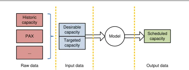
Fig. 1 Flow-chart of capacity requirements treatment in our model

robustness of services. Moreover, resulting schedules may include underused units, e.g. units only serving one or two trains as their daily workload because of the minimization of carriage-mileage. By appropriately keeping the capacity requirements for some OP trains at their (higher) historic schedule level, the underused train unit resources may be assigned to cover more trains, which makes the overall schedule more balanced. Therefore it is reasonable to adjust the capacity requirements to have some of the OP trains to set their capacity requirements as historic and the other as PAX. However which subset of trains should be so adjusted is a tricky issue for manual decision making.

On the other hand, for some instances the PAX levels for peak hour trains are too high such that the appearance of many UP trains is inevitable given a

limited fleet size. Nevertheless, a subsetSU P of the UP trains can be identified

to increase their capacity requirements from historic to PAX without violating the fleet size bound. However, it is also tricky to decide which subset of the UP trains to strengthen solely by a manual process.

Finally, it is possible that both OP and UP trains are present in manual schedules, making the problem more complicated.

4 Model and formulation

This paper proposes a novel TUSP integer multicommodity flow model that can achieve appropriate capacity provisions taking two levels of capacity re-quirements derived from raw capacity information such as capacity provisions in past operated schedules and PAX.

Let N be the set of trains in a given timetable. The first level of

capac-ity requirements is a target capaccapac-ity rj,∀j ∈ N that must be satisfied by

the model. The second level of capacity requirements is a desirable capacity

r′_j,∀j∈N that will be satisfied as much as possible but not mandatory. How

to convert raw data to the two levels of capacity requirements will be

problem-specific. A basic rule would be to always ensure that ρj ≤ ρ′j. For example,

rj= min(ρHj , ρPj) andrj′ = max(ρHj , ρPj). In this paper, all train capacities are

Figure 1 illustrates how different capacities are processed within the model. The raw data such as historic capacity provision and PAX will be converted into two levels of capacity requirements—a lower target capacity and a higher desirable capacity.

The proposed bi-level capacity requirement model is derived from the mod-els in Lin and Kwan (2013, 2014). It is based on a directed acyclic graph (DAG)

G= (N,A), where the node set N ={s, t} ∪N and the arc setA=A0∪A.

sand tare the source and sink nodes while N is the set of train nodes, each

representing a train servicej∈N in the timetable.A0is the set of sign-on/-off

arcs, that is, A0 = {(s, j) : j ∈ N } ∪ {(j, t) : j ∈ N }. Generally every train

node has a sign-on arc and a sign-off arc.Adenotes the set of connection-arcs

where a connection-arc a = (i, j) ∈ A links two train nodes i and j if it is

possible for i and j to be served consecutively by the same train unit. P is

used to denote the set of all s-t paths in G such that each p∈P represents

a sequence of trains as a workload plan for a unit. Moreover, Pj is used to

denote the set of paths passing through nodej.

As for the fleet, let K be the set of unit types, corresponding to the

com-modities in a multicommodity flow model. Type-graphs Gk _{= (N}k_,Ak_{) as}

sub-graphs of G are constructed with respect to each type k ∈ K generally

based on the principle that a type-graphGk _{will only contain train nodesN}k

(apart froms, tas mandatory) that are compatible with units of typek(and

arcs Ak _{to be constructed accordingly). The components of G}k _{will also be}

denoted in a similar way, e.g.Pk _{represents the set of paths inG}k_.

There are two kinds of decision variables:

– xp∈Z+,∀p∈Pk,∀k∈K represent the number of type-kunits used for a

workload plan given by pathpinGk_.

– yj∈R+,∀j∈N represent the capacity provision at trainj.

To satisfy target capacity requirements rj and coupling upper bound

con-straints as mentioned in Section 1 strictly, an enumeration on all possible unit

combinations is made for each train service (Lin and Kwan (2014)). LetKj be

the set of available types for trainj, and letwj= (wj1, w

j

2,· · ·, w

j

|Kj|)

T _∈ZKj

+

be a unit combination atj wherewj_k stands for the number of units of typek

used forj. A unit combination set is defined for eachj as

Wj := n

wj∈ZKj

+

∀w

j_{: a feasible unit combination for trainj}o_,∀j∈N,

(1) where the feasibility of unit combination is given by:

(i) P

k∈Kj

P p∈Pk

j qkxp≥rj, i.e. the target capacity requirementrjis strictly

satisfied for trainj, whereqk is the unit capacity of typekin number of

seats.

(ii) A unit combination assigned toj is within its coupling upper bound.

Then for each train j ∈ N, its corresponding train convex hull is computed based on its combination set as

conv(Wj) =

n

wj ∈RKj

+

H

j_wj_≤hjo_{,∀j∈N, (2)}

which is described by nonzero facets f ∈ Fj such that Hj ∈ RFj×Kj and

hj∈RFj. Via variable conversionwkj =

P p∈Pk

j xp, the passenger demand and

coupling upper bound requirements at trainjcan be satisfied by the following

train convex hull constraints

X

k∈Kj

X

p∈Pk j

H_f,kj xp≤hjf,∀f ∈Fj,∀j∈N. (3)

Having the above train convex hull constraints per train, we have problem

(P), the integer linear programming (ILP) formulation on the integer

multi-commodity flow model for the TUSP with two levels of capacity requirements as

(P) min C1

X

k∈K X

p∈Pk

cpxp+C2

X

j∈N yj−r

′

j

(4)

s.t. (3) and X

p∈Pk

xp≤bk0, ∀k∈K; (5)

X

k∈Kj

X

p∈Pk j

qkxp=yj, ∀j∈N; (6)

xp∈Z+, ∀p∈Pk,∀k∈K.

(7)

The first term in the objective function (4) is the sum of all the used

paths’ costs where cp is the weighted cost for path p with sub-weights on

different components. An overall weight C1 is set for it. Typically, cp

in-cludes sub-terms with respect to fleet size, carriage-mileage, empty-running

movements, and preferences. Specifically in our experiments for (P), cp =

CF ScF S_p +CCMP a∈Apc

CM

a +CER P

a∈Epc

ER

a is set. cF Sp is the fleet size

cost for using one unit and CF S _{is the sub-weight on fleet size. c}CM

a is the

carriage-mileage cost implied by arca formulated with preferences regarding

type-route, maintenance gap and so on,Apis the set of arcs in pathpandCCM

is the sub-weight on carriage-mileage. In our experiments, we use a simplified

setting as cCM

a = 1 for all arcs’ carriage-mileage costs. Therefore, regarding

carriage-mileage, we will simply report the number of used arcs in the

ex-periment section. cER

a is the cost of an empty-running movement when arca

implies such a movement, Ep is the set of empty-running arcs in path pand

CER is the empty-running sub-weight. The second term in (4) is the sum of

deviations between the desirable capacity and the solver’s real provision with

a weightC2. We will call the first term the “path cost term” and the second

Besides Constraints (3) as aforementioned, Constraints (5) ensure that

the deployed unit number per type k will not exceed its fleet size limit bk

0.

Constraints (6) define the solver’s capacity provision for each train j as yj.

Finally, Constraints (7) give the variable domains.

To overcome the non-linearity caused by the absolute value in the objective

function and to convert (P) into an LP, a conventional remedy is used. We

create a pair of variablesy+

j, y

−

j ,∀j∈N and take the replacement|yj−r′j|=

y_j++y−_j andyj−rj′ =y

+

j −y

−

j , ∀j ∈N in the original model. Therefore, in

the actual formulation, the OP deviation term in the objective function (4)

becomesC2P_j∈N(y

+

j+y

−

j ) and Constraints (6) become

P k∈Kj

P p∈Pk

j qkxp=

y_j+−y_j−+r′_j,∀j∈N.

Compared with the models in Lin and Kwan (2013, 2014), (P) has removed

the “fixed-charge” components, making it a standard integer multicommodity flow problem. This significantly improves the efficiency of the solution pro-cess. Furthermore, the remaining tasks to be achieved by the fixed-charge components in eliminating excessive coupling/decoupling and ensuring con-nection time allowance involving coupling/decoupling can be handled by post-processing as mentioned in Section 2 after solving the main ILP model. As the focus of this paper is on the bi-level capacity requirements, we choose

to not include the fixed-charge terms in (P). Similar strategies in achieving

the bi-level requirements can be applied to the full version with fixed-charge components by analogy.

To solve (P) exactly, a similar branch-and-price method as in Lin and Kwan

(2013, 2014) is used. The paths are dynamically generated by shortest path subproblems per traction type. Two customized branching methods named banned location branching and train-family branching are embedded into the relevant branch-and-bound (BB) tree. Banned location branching will identify LP-relaxation solutions at BB tree nodes with coupling/decoupling operations at locations banned for these activities and form branches to gradually remove them. Train-family branching will identify LP-relaxation solutions at BB tree nodes with incompatible unit types covering the same train and form branches to allow only compatible types at each child node. Appropriate post-processing on a station-by-station basis is used to eliminate excessive coupling/decoupling and remove unit blockage, yielding a finalized operable solution for train op-erating companies.

5 Computational experiments

Gourock Wemyss Bay

Kilwinning Largs

Ary

Troon Mount Florida

Neilston Balloch

Hyndland Patrick Milngavie

Queen’s Street

Larkhall Springburn Drumgelloch Cumbernauld Larbert Inverkeithing

Glasgow Central _Bathgate

North Berwick Whifflet Stranraer Shotts To Carlisle Newton

Motherwell _NewcastleTo Dalmuir To Dumfries, Carlisle Edinburgh Waverley Croy

Paisley Gilmour St

Lanark Carstairs Dunbar East Kilbride Ardrossan Harbour Kilmarnock Paisley Canal Helensburgh Central Newcraighall

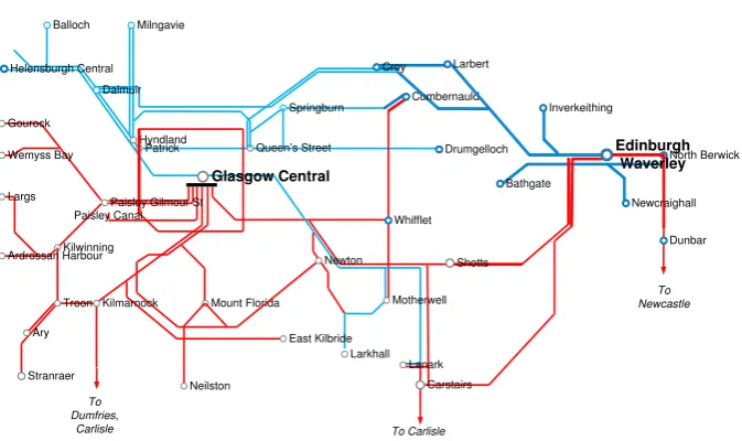
Fig. 2 Central Scotland railway network

5.1 Rail network and historic schedule

We performed experiments based on the datasets of the Central Scotland rail-way network (see Figure 2). We focus on the capacity provision and need a fast execution solver for experiments. For this reason and for the sake of simplicity, we have considered just one type of train unit in the following experiments. Table 1 gives a summary of the problem instance extracted for this train unit type. Since a single type of unit is concerned, train-family branching is no longer needed for experiments performed on this dataset and only banned location branching and the conventional fractional-to-integral branching are needed in the BB tree.

Table 1 Summary of problem instance

Number of origin/destination stations (among which coupling/decoupling is banned)

11 (6)

Operational period one working day

Fleet size 33

Number of train services 156

Train unit type Class 334 (183 seat capacity each)

In the December 2011 operated schedule provided by First ScotRail, all the demand of each of the 156 train services was satisfied by means of 33 train units, which results in 64 over-provided train services. From now on, we

will callOP the set of over-provided train services by comparing the historic

The experiments were conducted using a 64 bit Xpress-MP 7.7 package on a workstation with Intel Core i7-4790 CPU.

5.2 Experiments

Observe that the terms in the objective function (4) are competing. Minimiz-ing the OP deviation term implies augmentMinimiz-ing the fleet size and/or the current carriage-mileage (simplified to the number of used arcs in the experiments), which are part of the path cost term. The weights of the terms in the objec-tive function will then have a great impact on the resulting schedules and its calibration becomes an important issue.

First, we show the results by varying the weights of the objective function terms and observe that the same fleet size may over-provide different number

of trains. Second, in order to obtain the maximum number ofOP trains that

can be achieved within a certain fleet size, we fix parametrically an upper

bound for the fleet size and aim to minimize the deviation w.r.t.OP trains in

the existing schedule.

5.2.1 Varying weights in the objective function

We performed different iterations of model (P) by varying the C1 and C2

weights in (4), where C1+C2 = 1, and observe the impact of them in the

resulting train unit schedules. For that purpose, we gradually increase C2

and thereforeC1 will decrease accordingly, thus yielding a higher number of

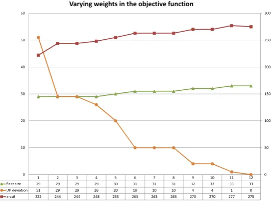
OP trains at each iteration. Results are presented in Table 2 and graphically

depicted in Figure 3. It can be observed that, as expected, the fleet size tends

to increase in order to reduce the OP deviation (measured in numbers of

trains in the table). On the other hand, the same fleet size may yield different

number ofOP, e.g. rows 1–4 in Table 2, the same fleet size of 29 train units

leads to different OP deviation in the interval from 26 to 51. In the fourth

column it can be seen that the number of arcs also increases when one aims to over-provide more trains within the same fleet size. This is affected by the fact that the same fleet size incur higher mileage in order to over-provide more trains.

The most important issue for the train operator is to minimize the fleet size while meeting all passenger demands and having as little deviation as possible from historic capacity provisions. According to these interests and the model results, the train operator is likely to select the option with the

minimum fleet size achieving the maximum possible number of OP trains,

that is, 29 train units and 38 OP trains corresponding to 26 OP deviation

Table 2 Varying weights in the objective function

C_{2 LP gap fleet size arcs# OP deviation ECS# time (sec) BBNode#}

0 0.03 29 222 51 1 62 98

0.02 0.3 29 244 29 1 49 54

0.05 0.8 29 244 29 1 37 69

0.1 0.63 29 248 26 1 1977 1562

0.13 1.55 30 255 20 1 51 71

0.14 0.56 31 263 10 1 392 613

0.15 0.39 31 263 10 1 124 167

0.16 0.22 31 263 10 1 60 63

0.17 0 32 270 4 1 60 38

0.18 0 32 270 4 1 53 31

0.5 1.48 33 277 1 2 38 28

1 0 33 276 0 2 37 27

1 2 3 4 5 6 7 8 9 10 11 12

fleet size 29 29 29 29 30 31 31 31 32 32 33 33

OP deviation 51 29 29 26 20 10 10 10 4 4 1 0

arcs# 222 244 244 248 255 263 263 263 270 270 277 275

0 50 100 150 200 250 300

0 10 20 30 40 50 60

Varying weights in the objective function

Fig. 3 Varying weights in the objective function (4)

w.r.t. the historic schedule and more than half of the trains in OP can still

remain over-provided.

5.2.2 Fixed fleet size

In order to obtain direct results on the maximum number ofOP trains that can

be achieved with a certain fleet size, we also performed experiments in which

the deviation with respect to the OP trains is minimized while establishing

that one can over-provide the complete OP set with 33 train units. From the previous results, it is known that 29 train units are sufficient to meet all passenger demands. We conducted experiments within these fleet size bounds respectively.

Results are presented on Table 3. As expected, when an upper bound is imposed on the fleet size, the fleet size achieved is equal to this upper bound.

For each value of the fleet size fixed, we obtain the best possibleOP from the

previous experiment.

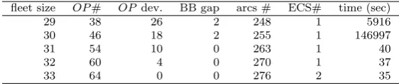
Table 3 Fixing scheduled fleet size from 29 to 33 train units. Resulting number of elements inOP

fleet size OP_# OP _{dev. BB gap arcs # ECS# time (sec)}

29 38 26 2 248 1 5916

30 46 18 2 255 1 146997

31 54 10 0 263 1 40

32 60 4 0 270 1 37

33 64 0 0 276 2 35

Observe that the computational complexity tends to increase as the fleet size decreases. The reason is that the smaller the number of train units, the higher the difficulty of over-providing train services. For most of the fleet size values (from 31–33), the stopping criterion was that the gap is less than one OP train, thus yielding a strict optimal solution. However, when the fleet size is equal to 29 or 30, no optimal solution could be obtained by this stopping criterion. We have created other stopping criteria for these cases, by setting a maximum number of BB nodes of 2000 for the fleet size of 29, and 12000 for the fleet size of 30. In both cases, the resulting BB gap (the difference between the imcubent integer solution’s objective value and the best BB tree lower bound) is equal to 2 OP trains.

6 Conclusions

We have introduced the train unit scheduling problem with bi-level, target and desired, capacity requirements. The first level concerns real passenger de-mands, which should be strictly satisfied, and the second level concerns historic capacity provisions that will be satisfied as much as possible. In the railway context it is often required to maintain the historic pattern of unit resource distribution wherever possible since this often contains implicit knowledge on agreements or expectations of transport authorities. Moreover this helps re-inforce the robustness of the schedule with respect to changes in passenger demands.

schedule. With the proposed method, all demands can be met with a 12% less fleet size and maintaining nearly the 60% most loaded train services within the over-provided ones in the historic capacity provisions.

A byproduct considering different levels of capacity requirements is that future expected demand growth may also be considered. This is especially rel-evant in the context of franchise bidding, where future growth in passenger demands should be taken into consideration. In this context, multi-level capac-ity requirements would be useful for scheduling considerations. Further work is to develop a multi-level capacity requirements model taking all the relevant aspects of franchise bidding into account.

Acknowledgements This research is supported by an EPSRC project EP/M007243/1. This support is gratefully acknowledged. We would like to also thank First ScotRail for their kind and helpful collaboration and for providing us data to support this study.

Data StatementWe acknowledge that First ScotRail has provided their operational data for the research, part of which is commercially sensitive. Where possible, the data that can be made publicly available is deposited inhttp://doi.org/10.5518/5.

References

Alfieri A, Groot R, Kroon LG, Schrijver A (2006) Efficient circulation of rail-way rolling stock. Transportation Science 40(3):378–391

Cacchiani V (2007) Models and algorithms for combinatorial optimization problems arising in railway applications. PhD thesis, University of Bologna, Italy

Cacchiani V (2009) Models and algorithms for combinatorial optimization problems arising in railway applications. 4OR, A Quarterly Journal of Op-erations Research 7(1):109–112

Cacchiani V, Caprara A, Toth P (2010) Solving a real-world train-unit assign-ment problem. Mathematical Programming B 124(1-2):207–231

Cacchiani V, Caprara A, Toth P (2012a) A Fast Heuristic Algorithm for the Train Unit Assignment Problem. In: Delling D, Liberti L (eds) 12th Workshop on Algorithmic Approaches for Transportation Modelling,

Opti-mization, and Systems, Schloss Dagstuhl–Leibniz-Zentrum f¨ur Informatik,

Dagstuhl, Germany, Open Access Series in Informatics (OASIcs), vol 25, pp 1–9

Cacchiani V, Caprara A, Toth P (2012b) Models and algorithms for the train unit assignment problem. In: Combinatorial Optimization, Lecture Notes in Computer Science, vol 7422, Springer Berlin Heidelberg, pp 24–35

Cacchiani V, Caprara A, Mar´oti G, Toth P (2013a) On integer polytopes with few nonzero vertices. Operations Research Letters 41(1):74–77

Fuchsberger M, L¨uthi PDHJ (2007) Solving the train scheduling problem in a main station area via a resource constrained space-time integer multi-commodity flow. Institute for Operations Research ETH Zurich

Jiang Z, Tan Y, Yalcinkaya O (2014) Scheduling additional train unit services on rail transit lines. Mathematical Problems in Engineering

Kroon LG, Lentink RM, Schrijver A (2008) Shunting of passenger train units: an integrated approach. Transportation Science 42(4):436–449

Lin Z, Kwan RSK (2013) An integer fixed-charge multicommodity flow (FCMF) model for train unit scheduling. Electronic Notes in Discrete Math-ematics 41:165–172

Lin Z, Kwan RSK (2014) A two-phase approach for real-world train unit scheduling. Public Transport 6(1):35–65

Mar´oti G (2006) Operations research models for railway rolling stock planning. PhD thesis, Eindhoven University of Technology, the Netherlands

Peeters M, Kroon LG (2008) Circulation of railway rolling stock: a branch-and-price approach. Computers & OR 35(2):538–556

Schrijver A (1993) Minimum circulation of railway stock. CWI Quarterly 6:205–217

Tracsis PLC (2013) TRACS-RS—rolling stock planning software. URL