Exact holomorphic differentials on a quotient of the Ree curve

This is a repository copy of Exact holomorphic differentials on a quotient of the Ree curve

.

White Rose Research Online URL for this paper:

http://eprints.whiterose.ac.uk/110213/

Version: Accepted Version

Article:

Dummigan, N. and Farwa, S. (2014) Exact holomorphic differentials on a quotient of the

Ree curve. Journal of Algebra, 400. pp. 249-272. ISSN 0021-8693

https://doi.org/10.1016/j.jalgebra.2013.11.016

Article available under the terms of the CC-BY-NC-ND licence

(https://creativecommons.org/licenses/by-nc-nd/4.0/)

[email protected] https://eprints.whiterose.ac.uk/

Reuse

This article is distributed under the terms of the Creative Commons Attribution-NonCommercial-NoDerivs (CC BY-NC-ND) licence. This licence only allows you to download this work and share it with others as long as you credit the authors, but you can’t change the article in any way or use it commercially. More

information and the full terms of the licence here: https://creativecommons.org/licenses/

Takedown

If you consider content in White Rose Research Online to be in breach of UK law, please notify us by

Exact holomorphic differentials on a quotient of the Ree

curve.

Neil Dummigan, Shabieh Farwa∗

September 9, 2013

Abstract

We produce several families of exact holomorphic differentials on a quotientX

of the the Ree curve in characteristic 3, defined byX : yq_−y=xq0_(xq_−x)/F q,

(whereq0= 3s, s>1 andq= 3q 2

0). We conjecture that they span the whole space

of exact holomorphic differentials, and prove this in the casess= 1 and s= 2, by calculating the kernel of the Cartier operator.

§1 Introduction

For a nonsingular projective curve C over a field K,H0_(C,Ω1_{) is the K-vector space}

of holomorphic (i.e. everywhere regular) differentials on C (defined over K). Such a differential is said to beexactif it is of the formdf for some functionf ∈K(C). Iff is constant thendf = 0. Iff is non-constant thenf necessarily has at least one pole, and ifK has characteristic 0 thendf will have a pole in the same place. So in characteristic 0, there are no non-zero exact holomorphic differentials. But in characteristic p > 0, wherepth_{powers differentiate to 0, a pole whose order is a multiple ofpmight disappear}

upon differentiation, and there can be non-zero exact holomorphic differentials. Inside H0(C,Ω1), the subspace of exact holomorphic differentials is the kernel of the Cartier operatorC_{. It seems like a natural problem, given a curveC/K with char(K) =p > 0,} to calculate this subspace. There are at least two further ways to motivate this problem.

First, dimKH0(C,Ω1)C=0 = dimKHom(αp, JC[p]), the so-called a-number of the Jaco-bian JC of C [LO, Equation 5.2.8]. Here JC[p] is the sub-group-scheme of p-torsion,

∗

N. Dummigan, School of Mathematics and Statistics, University of Sheffield, Hounsfield Road, Sheffield, S3 7RH, U.K. ([email protected]).

andαp≃Spec(K[x]/xp) is the group-scheme ofpth-roots of 0. Note that each element b∈K gives an endomorphism of αp, via x7→ bx, so Hom(αp, JC[p]) is naturally a K-vector space. Thisa-number is an important invariant ofJC[p]. For instance,a+f ≤g, wheref = dimFp(JC[p](K)) is the “p-rank” ofJC. For more, see [FGMPW], [LO].

Second, suppose that K is finite, that E/K is an elliptic curve, and consider E as a “constant” elliptic curve over the global field K(C). Then morphisms from C to E, defined overK, are identified withK(C)-rational points ofE. It may happen that αp is isomorphic to a subgroup-scheme ofE[p], necessarily kerF :E →E(p), the kernel of thepth_{-power Frobenius morphism. In fact, this is always true whenEis supersingular}

(in which case the kernel of the Verschiebung V : E(p) → E is also isomorphic to αp). Then the Selmer group for the isogeny F is identified with the flat cohomology H1_{(C, α}

p), which in turn is identified with H0(C,Ω1)C=0, [U, Proposition 3.3(b)]. For a supersingularE/K, an invariant differentialω (on any isogenous curve) is exact, and if θ: C → E(p) is a K(C)-rational point on E(p) then the pullback θ∗

(ω) is an exact holomorphic differential on C. In this way E(p)_{(K(C))/F(E(K(C))) is embedded as}

a subgroup ofH0(C,Ω1)C₌₀

, and the cokernel is theF-torsion in the Shafarevich-Tate group ofE/K.

Friedlander et. al. [FGMPW] calculate the space of exact holomorphic differentials on the Suzuki curve C :yq−y =xq0_(xq_{−x), with q = 2q}2

0,where q0 = 2s, s ≥1, of

genusg=q0(q−1), in order to determine the a-number of its Jacobian. The fact that

the characteristic is 2 ensures that the exact differentials are simply those of the form f2dx, and one just has to find a basis for thosef with divisor bounded such thatf2dx is holomorphic.

Gross [G] calculates the space of exact holomorphic differentials on the Hermitian curve C:yq+1=xq+x /Fq2, (whereq =pf is a prime power), of genusg=q(q−1)/2, in order

to bound from below the order of the Shafarevich-Tate group, and thereby to improve a bound for the sphere-packing density of the Mordell-Weil lattice E(K(C))/const ≃ HomK(JC, E). (This free, finitely-generated abelian group has on it an even integral quadratic form, given by twice the degree of a morphism. This construction of lattices is due to Elkies.) The finite group F×_q2 acts on C/Fq2 by the automorphisms (x, y) 7→

(αq+1x, αy), and this abelian group action decomposes H0(C,Ω) into one-dimensional pieces (spanned byxm_yn_{dywithm, n≥0 andm+n≤q−2) on which the group acts by} distinct characters. The Cartier operator necessarily permutes these one dimensional spaces, so to find its kernel one only needs to know which of these basis elements it kills, so again the calculation is relatively simple.

The Suzuki curve enjoys automorphisms by the finite simple group Sz(q) =2B2(q),

while the Hermitian curve is acted upon by a finite projective unitary group PU3(q).

The third family of Deligne-Lusztig curves (see [H]) comprises those acted upon by the finite simple Ree groups2G2(q), whereq = 3q02,with q0= 3s, s≥1. The function field

of the Ree curveC′

/Fq is given by Fq(C′

) =Fq(x, y1, y2), with

yq₁−y1 =xq0(xq−x) (1)

yq₂−y2 =xq0(yq₁−y1). (2)

The genus of C′

is g = 3₂q0(q−1)(q +q0 + 1), and it has 1 +q3 Fq-rational points,

including one point at infinity. LetX (of genus 3₂q0(q−1)) be the non-singular model

of the function field of the affine curve defined by (1). It is a quotient ofC′

/Fq, via the mapπ :C′

→X such that (x, y1, y2)7→(x, y1). From now on, for the sake of simplicity

we will replacey1 by y, so (the function field of) X is defined by the equation

yq−y=xq0_(xq_{−x). (3)}

We seek the exact holomorphic differentials for the quotientX rather than for the Ree curve itself, since it seems to be a more tractable problem. (We are grateful to the referee for pointing out that for the Ree curve, even an explicit basis forH0(C′,Ω1) is not known.) Furthermore, X is a direct analogue of the Suzuki curve, being defined by an equation that looks the same. For both X and the Suzuki curve there is an action of F×q, by (x, y) 7→ (αx, αq0+1y), but unlike the Hermitian case, this does not decomposeH0(X,Ω1) into one-dimensional eigenspaces. Despite this, the Suzuki curve may be dealt with fairly easily because the characteristic is only 2. The source of the extra difficulty in characteristic 3 is identified in Remark 1, in Section 3. For more on quotients ofX, see [CO1, CO2].

Conjecture 1.1. Let q0 = 3s, q = 3q02, with s ≥ 1, and let X/Fq be a complete

nonsingular model of the curve yq _{−y = x}q0_(xq _{−x). The dimension of the space}

H0_(X,Ω1₎C₌₀

, of exact holomorphic differentials on X, is

d:= 2q0 27 14q

2 0+ 9

+ 1 12 11q

2 0+ 9

.

Theorem 1.2. d is a lower bound for the dimension of H0_(X,Ω1₎C₌₀

(i.e. for the a-number of the Jacobian of X), for all s≥1.

Theorem 1.3. In the casess= 1ands= 2,dis equal to the dimension ofH0(X,Ω1)C₌₀ .

We should make some remark on one of the motivating problems. The zeta function of X/Fq is

(1 + 3q0t+qt2)q0(q−1)(1 +qt2)q0(q−1)/2

(1−t)(1−qt) .

LetE1, E2/Fq be elliptic curves with zeta functions

(1 + 3q0t+qt2)

(1−t)(1−qt) and

respectively. LettingLi = HomK(JX, Ei), fori= 1,2, we find that rank(L1) = 2q0(q−

1) and rank(L2) =q0(q−1), and that JX is isogenous to Eq0(q −₁₎

1 ×E

q0(q−_1)/2

2 . This

isogeny is not an isomorphism, and fors= 1 or 2 a simple reason is that our calculations show that a6=g. In what follows, we omit details, but see the proofs of Propositions 11.11 and 14.10 of [G] for the method by which ranks are calculated, minimal norms bounded from below and determinants bounded from above. Note that for the refined upper bound for the determinant of the lattice, a lower bound for dimH0(X,Ω1)C₌₀ is required, which is precisely what we have. Let the centre density of a lattice L of rank nbe δ := (min_(det/_L4)₎1n//22, where min is the minimal norm. This is the sphere-packing

density divided by the volume of a unit n-dimensional sphere. For L1, for s = 1 we

have n = 156 and find log₂(δ) ≥ −80.9, while for s = 2 we have n = 4356 and find log₂(δ) ≥710. For comparison, looking at records for known dense lattices in nearby dimensions in Table 1.3 of [CS], for n = 150, log₂(δ) = 113.06 and for n = 4098, log₂(δ) = 11279. ForL2 our bounds are even worse compared to record known lattices.

Still, it seems to be an interesting problem to determine invariants of these lattices. In the case of the Hermitian curve, the precise determinants are calculated in [D1], while the structure of the Shafarevich-Tate group is obtained in [D2].

In Section 2 we introduce useful functionsuandv onX, and find a basis for the space of holomorphic differentials onX, comprising certain elements of the formxaybucvddx, with 0 ≤ b ≤ 2 and various restrictions on the other exponents. In Section 3 we introduce the Cartier operator, and calculate its action on the 81 differentials of the form ω=xα_yβ_uγ_vδ_{dxwith 0≤α, β, γ, δ ≤2. SinceC(f}3_{ω) =fC(ω), this determines}

which of our basis elements are exact. In Section 4 we prove Theorem 1.2 by producing as many exact holomorphic differentials as we can. In Section 5 we consider a natural action of the group_F×

q onH0(X,Ω1), and show that the eigenspaces are of dimensions

3q0±1

2 . The Cartier operator permutes these eigenspaces, so we may consider its kernel

on each separately. In Section 6, we prove Theorem 1.3 by calculating these kernels in the cases s = 1 and s= 2. Throughout the paper, we work over K =Fq, but the calculations look exactly the same over any extension.

We thank the anonymous referee for their thoughtful reading, and their help in improv-ing both the organisation and the substance of this paper.

§2 The holomorphic differentials on X

Recall thatX/Fq is a nonsingular projective model of the affine curveyq−y=xq0_(xq₋

x), where q0 = 3s and q = 32s+1,s≥1.

Proposition 2.1. X/Fq is irreducible with a single point at infinity (i.e. in the com-plement of the affine curve), denoted by P∞. The rational functions on X/Fq, defined by

are regular onX\ {P∞}. At P∞, the pole orders of these functions are

−ord∞(1) = 0, −ord∞(x) =q, −ord∞(y) =q+q0,

−ord∞(u) =q+ 3q₀, −ord∞(v) = 2q+ 3q₀+ 1.

The element xu_v is a uniformizer at P∞.

We omit the proof, since it is elementary, and essentially identical to that of Lemma 1.8 of [HS].

The pullback ofuto the Ree curveC′ is among the functions defined by Pederson [P], who calls itω1. (All rational functions onC′ that do not involvey2 may be considered

functions onX.) We have had to introducevhere for our purposes, but it is analogous to the function on the Suzuki curve denotedfq+2q0+1 by Hansen and Stichtenoth [HS].

From the above definitions of u and v, one can easily verify the following relations in Fq(X):

y3 =x2u+v; (4)

uq0 _=xq0_{x−y; (5)}

vq0 _=x2q0_{y−u . (6)}

Proposition 2.2. The curve X has genus g = 3₂q0(q −1). The differential dx has

divisordiv(dx) = (2g−2)P∞.

Proof. If (α, β)∈X(Fq)\ {P∞}, thenβ is one of theq roots of the equation

yq−y =αq0_(αq_−α).

Ifh(y) :=yq_−y−αq0_(αq_{−α), then h and} dh

dy have no common roots, so all the roots ofyq−y=αq0_(αq_{−α) are distinct. Thus we haveq distinct points for which (x−α)}

is zero. But−ord∞(x−α) =−ord∞(x) =q, so all of these zeros are simple zeros, and hence

ord(α,β)dx= ord(α,β)d(x−α) = 0,

showing that dxhas no zeros on X(Fq)− {P∞}. Since deg(div(dx)) = 2g−2 ,

div(dx) = (2g−2)P∞. (7)

Now we find the genus. Fromv =x2y3q0_−u3q0 _{we get}

dv= 2xy3q0_dx

⇒ord∞(dx) = ord∞(dv)−ord∞(x)−ord∞(y3q0). (8)

Since −ord∞(v) is coprime to 3, −ord∞(dv) =−ord∞(v) + 1 = 2q+ 3q₀+ 2. Putting this in (8) gives

But (7) shows that ord∞(dx) = 2g−2. Comparing with (9) gives

g= 3

2q0(q−1)

Define a set I of indices (a, b, c, d)∈Z4 by the following conditions:

1. a, b, c, d≥0.

2. a+b+c+ 2d≤3q0−1.

3. Ifa+b+c+ 2d= 3q0−2 then 0≤c≤2q0−2. Writing c= 2q0−2−i, where

0≤i≤2q0−2, either (i) b+ 3d <2 + 3iand d≤ q0+₂ i or (ii)b+ 3d= 2 + 3iand

0≤d≤q0−2.

4. Ifa+b+c+2d= 3q0−1 then 0≤c≤q0−2. Writingc=q0−2−j, b+3d≤2+3j.

Lemma 2.3. The differential xaybucvddx is holomorphic if and only if (a, b, c, d)∈I.

This can be checked using Propositions 2.1 and 2.2

Proposition 2.4. DefineJ ={(a, b, c, d)∈I | 0≤b≤2 and 0≤c, d≤q0−1}. Then

{xaybucvddx| (a, b, c, d)∈J} is a basis for H0(X,Ω1).

Proof. The holomorphic differentialsxaybucvddx, for (a, b, c, d)∈J, have distinct orders at P∞. (See the proof of Proposition 3.7 of [FGMPW], which is the characteristic 2 analogue.) Hence they are linearly independent. If one counts the elements of J, there are exactlygof them, hence the corresponding differentials must form a basis for H0_(X,Ω1_).

§3 Exact differentials and the Cartier operator

LetK be a field of characteristicp >0, andC/K any nonsingular projective curve. We will use the (non-linear) Cartier operatorC_{, which maps the space ΩC of meromorphic} differentials onC to itself.

Proposition 3.1. Some of the properties of the Cartier operator are as follows [S, Section 10].

(1) If ν is not a pth _{power in the function field K(C), then every f ∈ K(C) can be}

expressed as

f =f₀p+f₁pν+...+f_pp−₁νp

−1 ₍₁₀₎

for suitablefi ∈K(C). We define

(2)C _{is well-defined, independent of the choice of ν.}

(3)C _{is additive:} C_{(ω1+ω2) =}C_{(ω1) +}C_{(ω2) for all ω1, ω2 ∈ΩC.}

(4) For any differential ω on C andg∈K(C), C_(gp_{ω) =g}C_(ω).

(5)C_{(ω) = 0 if and only if ω is exact.}

Proposition 3.2. The exact meromorphic differentials onX/Fq are precisely those of the form

ω= (f₀3+f₁3x)dx, for f0, f1 ∈Fq(X). (12)

Proof. It is clear that x is not a cube in Fq(X), as if it were then so would be y, by (3), so every function inFq(X) would be a cube, which is not true of course, asFq(X) is not perfect. (Alternatively, as suggested by the referee, we can see from Proposition 2.1 that the pole order ofv is not divisible by 3.) Now from Proposition 3.1(1) we can write every functionf ∈Fq(X) as

f =f₀3+f₁3x+f₂3x2, (13)

and C_{(f dx) =f2dx, so by Proposition 3.1(5), ω =f dx is exact if and only if it is of} the form

ω= (f₀3+f₁3x)dx.

(Observe how one can “integrate” such a differential without trying to divide by zero.)

Remark 1: There is a possibility that cancelation of poles takes place between the two terms f₀3dx and f₁3x dx. The difficulty this causes, in determining which exact differentials are holomorphic, does not arise in the characteristic 2 case, where there is only one term (f₀2d ν) in the expression for an exact differential. To find a basis for the exact holomorphic differentials on the Suzuki curve, one simply takes {f₀2d x}, where f0 runs through a basis for L((g−1)P∞) ={f ∈K(C)|div(f)≥ −(g−1)P∞}.

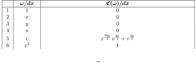
Recall (from Proposition 2.4), a basis for the space of holomorphic differentials on X, involving certain xaybucvddx. Each is a cube times one of the 81 things given by xα_yβ_uγ_vδ_{dx, with 0≤α, β, γ, δ ≤2. So if we know how the Cartier operator applies} to these 81 differentials then we know how it applies to any element in the basis.

[image:8.612.65.460.596.723.2]

Proposition 3.3. If ω =xα_yβ_uγ_vδ_{dx, with 0≤α, β, γ, δ ≤2, thenC(ω) is given by} Table 1 below.

ω/dx C_(ω)/dx

1 1 0

2 x 0

3 y 0

4 u 0

5 v x2q30 u

q0 3 +v

q0 3

7 y2 x2q30

8 u2 _x2q0

9 v2 _x5q0

3 +1u q0

3 +xq0+1v q0

3 −x 2q0

3 y u q0

3 −y v q0

3

10 xy xq30

11 xu xq0

12 xv 0

13 yu x4q30

14 yv −x2q30 u

2q0 3 −u

q0 3 v

q0 3

15 uv −x4q30 u 2q0

3 +x 2q0

3 u q0

3 v q0

3 −v 2q0

3

16 x2y −uq30

17 x2u −x2q30 u

q0 3 −v

q0 3

18 x2_{v −x}q0_x+y

19 xy2 xq30 u

q0 3

20 y2u −x2q30 v

q0 3

21 y2v u2q30 v

q0 3

22 xu2 x5q30 u

q0

3 +xq0v q0

3

23 yu2 _x4q0

3 v q0

3

24 u2v x2q0_y−u

25 xv2 _x4q0 3 +1u

2q0 3 −x

2q0 3 +1u

q0 3 v

q0 3 +x v

2q0 3

26 yv2_{x x}q0+1_uq0 3 v

q0 3 +x

2q0 3 y u

2q0 3 +x

q0 3+1v

2q0 3 +y u

q0 3 v

q0 3

27 uv2x x4q30 y u 2q0

3 −x 2q0

3 y u q0

3 v q0

3 +y v 2q0

3

28 xyu xq0_uq30 −x q0

3 v q0

3

29 xyv −x4q30+1+x q0

3 y

30 xuv −x2q0+1_+xq0_y

31 yuv −x2q30 u 2q0

3 v q0

3 +u q0

3 v 2q0

3

32 x2y2 u2q30

33 x2u2 x4q30 u 2q0

3 −x 2q0

3 u q0

3 v q0

3 +v 2q0

3

34 x2v2 x2q0+2+xq0+1y+y2

35 y2u2 x2q30 v

2q0 3

36 y2v2 x5q30+1y−x 2q0

3 y2+x q0

3+1u q0

3 v 2q0

3 −y u 2q0

3 v q0

3

37 u2v2 x2q0_y2_+xq0+1_u+yu

38 x2yu x2q30 u 2q0

3 +u q0

3 v q0

3

39 x2yv −xq0+1_uq₃0 _+xq₃0+1_vq₃0 _{−y u}q₃0

40 x2_{uv −x}5q0 3 +1u

q0

3 −xq0+1v q0

3 −x 2q0

3 y u q0

3 −y v q0

3

41 xy2_{u −x}q0

3 u q0

3 v q0

3

42 xy2v x2q30+1v q0

3 +x q0

3 y u q0

3

43 y2uv x4q30 y u q0

3 +x 2q0

3 y v q0

3 −u 2q0

3 v 2q0

3

44 xyu2 xq0_u

q0 3 v

q0 3 +x

q0 3 v

2q0 3

45 xu2_{vx x}5q0

3 y u q0

3 +xq0y v q0

46 yu2v −x4q30 y v q0

3 +u q0

3 +1

47 xyv2 −x4q30+1y+x 2q0

3 +1u 2q0

3 v q0

3 +x q0

3 y2−x u q0

3 v 2q0

3

48 xuv2 _x2q0+1_y+xq0_x2_+xu

49 yuv2 −x4q30y2+x 2q0

3 y u 2q0

3 v q0

3 +x q0

3+1u−y u q0

3 v 2q0

3

50 xyuv −x4q30+1v q0

3 +xq0_{y u} q0

3 −x q0

3 y v q0

3

51 x2y2u x2q30 y−u 2q0

3 v q0

3

52 x2_y2_{v x}q0

3 +1u q0

3 v q0

3 +y u 2q0

3

53 x2_yu2 _x4q0 3 y+x

2q0 3 u

2q0 3 v

q0 3 −u

q0 3 v

2q0 3

54 x2u2v x4q30 y u 2q0

3 −x 2q0

3 y u q0

3 v q0

3 +y v 2q0

3

55 x2yv2 x4q30+2v q0

3 +xq0+1y u q0

3 −x q0

3 +1y v q0

3 −y2u q0

3

56 x2uv2 x5q30+1y u q0

3 +xq0+1y v q0

3 −x 2q0

3 y2u q0

3 −y2v q0

3

57 xy2u2 x5q30 y+x q0

3 u q0

3 v 2q0

3

58 y2_u2_{v x}2q0 3 y v

2q0 3 −u

2q0 3 +1

59 xy2v2 −x4q30+1y u q0

3 +x q0

3 y2u q0

3 +x u 2q0

3 v 2q0

3

60 y2uv2 −x4q30+1y2u q0

3 +x q0

3+1u q0

3+1+ y u 2q0

3 v 2q0

3

61 xu2v2 x5q30 y2u q0

3 +xq0_y2_v q0

3 −x 2q0

3 +1u q0

3+1−x u v q0

3

62 yu2v2 x4q30 y2v q0

3 +xq0+1u q0

3+1−x q0

3+1u v q0

3 −y u q0

3+1

63 x2_{yuv −x}q0+1_uq0 3 v

q0 3 +x

2q0 3 y u

2q0 3 −x

q0 3+1v

2q0 3 +y u

q0 3 v

q0 3

64 xy2_{uv −x}2q0 3 +1v

2q0 3 −x

q0 3 y u

q0 3 v

q0 3

65 xyu2v xq0_{y u}q30 v q0

3 +x q0

3 y v 2q0

3

66 xyuv2 x4q30+1y v q0

3 +xq0_y2_u q0

3 −x q0

3 y2v q0

3 −x u q0

3+1

67 x2y2u2 −x4q30 y u q0

3 +x 2q0

3 y v q0

3 +u 2q0

3 v 2q0

3

68 x2_y2_v2 _x2q0 3 +2v

2q0 3 −x

q0 3+1y u

q0 3 v

q0

3 +y2u 2q0

3

69 x2_u2_v2 _x4q0 3 y2u

2q0 3 −x

2q0 3 y2u

q0 3 v

q0 3 +y2v

2q0 3

70 y2u2v2 x2q30 y2v 2q0

3 −x q0

3+1u q0

3+1v q0

3 +y u 2q0

3 +1

71 x2y2uv −x5q30+1y+x 2q0

3 y2−x q0

3+1u q0

3 v 2q0

3 −y u 2q0

3 v q0

3

72 x2yu2v x4q30 y2+x 2q0

3 y u 2q0

3 v q0

3 −x q0

3+1u−y u q0

3 v 2q0

3

73 x2_yuv2 _xq0+1_{y u}q₃0 _vq₃0 _−x 2q0

3 y2u 2q0

3 +x q0

3+1y v 2q0

3 −y2u q0

3 v q0

3

74 xy2_u2_{v x}5q0

3 y2−x 2q0

3 +1u+x q0

3 y u q0

3 v 2q0

3

75 xy2uv2 x2q30+1y v 2q0

3 −x q0

3 y2u q0

3 v q0

3 +x u 2q0

3 +1

76 xyu2v2 xq0_y2_uq30 v q0

3 +x 2q0

3 +1u 2q0

3 +1+x q0

3 y2v 2q0

3 +x u q0

3+1v q0

3

77 x2y2u2v −x4q30y2u q0

3 +x 2q0

3 y2v q0

3 −x q0

3 +1u q0

3 +1+y u 2q0

3 v 2q0

3

78 x2y2uv2 x5q30+1y2+x 2q0

3 v+x q0

3 +1y u q0

3 v 2q0

3 −y2u 2q0

3 v q0

3

79 x2y_u2_v2 _−x4q0

3 +2u+x 4q0

3 v+x 2q0

3 y2u 2q0

3 v q0

3 +x q0

3+1y u−y2u q0

3 v 2q0

3

80 xy2_u2_v2 _x5q0

3 +2u+x 5q0

3 v−x 2q0

3 +1y u+x q0

3 y2u q0

3 v 2q0

3 4−x u 2q0

3 +1v q0

3

81 x2y2u2v2 −x4q30+2u q0

3+1−x 4q0

3 u q0

3 v+x 2q0

3 v q0

3+1+x q0

3 +1y u q0

3+1+

y2u2q30v 2q0

Table 1: The Cartier Operator

Proof. In order to apply the Cartier operator, we first express each f = xα_yβ_uγ_vδ_, with 0≤α, β, γ, δ ≤2, in the form f =f₀3+f₁3x+f₂3x2. For this recall (5) and the definitions of uand v:

y=uq0_−xq0_{x; (14)}

u=x3q0_x−y3q0_{; (15)}

v=y3q0_x2_−u3q0_{. (16)}

Using these relations, we can express all of the above 81 monomials in the form

f =f₀3+f₁3x+f₂3x2.

For 1 and x, it is obvious that f3

2 = 0, thereforeC(dx) =C(x dx) = 0. Similarly from

(14),

y dx= [(uq30)3−(x q0

3 )3x]dx. (17)

In the above equationf0 =u q0

3 andf₁ =x q0

3 , whilef₂ = 0, so consequentlyC(ydx) = 0.

Similarly, C(u dx) = 0. Also, (16) shows that

v dx= [(−uq0₎3_{+ (y}q₃0₎3_x2_{]dx. (18)}

Thusf2 =y q0

3 , soC(vdx) =y q0

3 dx, which shows thatv dx is not exact. However if we

consider xv dx, then from

xv dx= [(xyq30)3−(uq0)3x]dx, (19)

it is clear thatf2 = 0, thereforeC(xv dx) = 0, soxv dx is an exact differential.

We give just one more complicated example to illustrate how the results in the table were obtained. We show how to calculate entry 35.

From (14) and (15), we have

y2u2dx= [x7q0+3uq0_+x5q0+3_y3q0_+y6q0_u2q0_]dx

+ [x8q0+3+x3q0_y3q0_u2q0_+xq0_y6q0_uq0_{]x dx}

+ [x6q0_u2q0 _+x4q0_y3q0_uq0 _+x2q0_y6q0_]x2_dx.

From the above equation, f₂3 fory2u2 is

f₂3= [x2q0_u 2q0

3 +x 4q0

3 yq0u q0

3 +x 2q0

3 y2q0]3.

Hence

C(y2u2dx) = [x2q0_u 2q0

3 +x 4q0

3 yq0u q0

3 +x 2q0

The above expression involvesyq0_dxandy2q0_{dx, which are not in the basis forH}0_(X,Ω1₎

in Proposition 2.4, so we need to replace them using (4):

y3 =x2u+v ⇒ (y3₎q0

3 = (x2u+v) q0

3

⇒ yq0 _{= (x}2_u)q₃0 _{+ (v)}q₃0_{. (21)}

Putting these values in (20), we have

C_(y2_u2_{dx) =[x}2q0_u 2q0

3 +x 4q0

3 u q0

3 (x 2q0

3 u q0

3 +v q0

3 ) +x 2q0

3 (x 4q0

3 u 2q0

3 −x 2q0

3 u q0

3 v q0

3 +v 2q0

3 )]dx

=[x2q0_u 2q0

3 +x2q0u 2q0

3 +x 4q0

3 u q0

3 v q0

3 +x2q0u 2q0

3 −x 4q0

3 u q0

3 v q0

3 +x 2q0

3 v 2q0

3 ]dx

=x2q30 v 2q0

3 dx.

The table shows in particular that among the 81 differentials considered, the only exact ones are dx,x dx,y dx,u dxand xv dx. The exactness of these differentials may be verified directly: dx = d(x), x dx = d(−x2_{), y dx = d(−u}q0_{x −x}q0_x2_{), u dx =}

d(x2q0_xy−vq0_{x) and xv dx = d(x}3_yq0_x+uq0_x2_{). The expressions for y dx, u dx and}

xv dx, may be verified easily using (4), (5) and (6).

§4 Proof of Theorem 1.2

We define certain classes Ai, Bi, Ci, Di of exact holomorphic differentials. That denoted “g dx” consists of all differentials f3g dxwith f =xαuγvδ; 0≤γ, δ≤ q0

3 −1,

with whatever further condition on α, γ and δ is necessary to make the differentials ω =f3gdx holomorphic. We will make these conditions explicit later, while counting the number of differentials in each of these classes.

A1: dx, A2: x dx, A3: y dx, A4: u dx, A5: xv dx.

Although y3dx is an exact holomorphic differential, it is not in the basis in Proposi-tion 2.4. However, from (4) we may express it in terms of the basis differentials as y3dx = (x2u+v)dx. This illustrates the fact that an exact differential may be a lin-ear combination of non-exact basis elements. Similarly we need to express each of the following exact holomorphic differentials in terms of the basis elements:

uq0_{dx, u}2q0_{dx, v}q0_dx

y3dx, y3uq0_{dx, y}3_u2q0_{dx, y}3_vq0_dx

In fact, we need to look at all of the above multiplied by each of 1, x, y, u and xv (55 possibilities). Although y9dx is an exact holomorphic differential, we do not consider y9_{dx, since}

y9dx=x6u3dx+v3dx,

which is a linear combination of differentials in classA1. In a similar way we can ignore the differentials involving the higher cubic powers of y. Thus we obtain the following classes.

B1: y3dx= (x2u+v)dx, B2: y3ydx= (x2yu+yv)dx, B3: y3_{udx= (x}2_u2_+uv)dx,

B4: y3xvdx= (x3uv+xv2)dx, B5: y6dx= (x3xu2−x2uv+v2)dx, B6: y6_{ydx= (x}3_xyu2_−x2_yuv+yv2_)dx,

B7: uq0_{xdx= (x}q0_x2_−xy)dx,

B8: uq0_{ydx= (x}q0_xy−y2_)dx,

B9: uq0_{udx= (x}q0_xu−yu)dx,

B10: uq0_{xvdx= (x}q0_x2_v−xyv)dx,

B11: uq0_y3_{ydx = (x}q0+3_yu+xq0_xyv−x2_y2_u−y2_v)dx,

B12: uq0_y3_{udx= (x}q0+3_u2_+xq0_xuv−x2_yu2_−yuv)dx,

B13: uq0_y3_{xvdx= (x}q0+3_xuv+xq0_x2_v2_−x3_yuv−xyv2_)dx,

B14: uq0_y6_{ydx = (x}q0+3_x2_yu2 _−xq0+3_yuv+xq0_xyv2_−x3_xy2_u2 _+x2_y2_uv−y2_v2_)dx.

Similarly with the help of the remaining possibilities (among those 55, stated earlier), we define some other classes of exact holomorphic differentials as follows.

y6udx= (x3u3x−x2u2v+uv2)dx

=x3u3xdx−(x2u2v−uv2)dx.

Sincex3u3xdx is already on A2, a new list of exact differentials is (denoted by) y6udx⇒C1: (x2u2v−uv2)dx.

Note that discardingx3_u3_{xdxreduces the pole order, allowing more possibilities forf}3_.

Similarly we just state the other such classes. All of the the following classes are obtained by discarding one (previously defined) differential, except for C14, which is obtained by discarding two differentials, belonging toB8and C4.

u2q0_{xdx⇒ C2: (x}q0_x2_y+xy2_)dx,

u2q0_{udx⇒ C3: (x}2q0_v−xq0_xyu−y2_u)dx,

vq0_{xdx⇒ C4: (x}q0_y2_−xu)dx,

vq0_{xvdx⇒ C6: (x}q0_x2_y2_u+xq0_y2_v−x3_u2_−xuv)dx,

y3u2q0_{xdx⇒ C7: (x}q0+3_xyu+xq0_x2_yv+x3_y2_u+xy2_v)dx,

y3u2q0_{udx⇒ C8: (x}2q0_x2_uv+x2q0_v2_−xq0+3_yu2_−xq0_xyuv−x2_y2_u2_−y2_uv)dx,

y3vq0_{udx⇒ C9: (x}2q0_yuv+x2q0−3_xyv2_v−xq0_xy2_u2_+xq0−3_x2_y2_uv−xq0−3_y2_v2_+u3_x2_+u2_v)dx,

y3vq0_{xvdx⇒ C10: (x}q0+3_xy2_u2_−xq0_x2_y2_uv+xq0_y2_v2_−x3_u3_x2_+x3_u2_v−xuv2_)dx,

y6uq0_{udx⇒ C11: (x}q0+3_u2_v−xq0_xuv2_−x2_yu2_v+yuv2_)dx,

y6u2q0_{xdx⇒ C12: (x}q0+6_yu2_−xq0+3_xyuv+xq0_x2_yv2_+x3_x2_y2_u2_−x3_y2_uv+xy2_v2_)dx,

y6u2q0_{udx⇒ C13: (x}2q0+3_xu2_v−x2q0_x2_uv2_+xq0+3_yu2_v−xq0_xyuv2_+x2_y2_u2_v−y2_uv2_)dx,

y6vq0_{udx⇒ C14: (x}2q0_x2_yu2_v−x2q0_yuv2_−u3_x2_v+u2_v2_)dx.

Among the 55 possibilities stated earlier, we may discard the remaining ones, as they are linear combinations of previously determined classes, e.g. y3_{xdx = (x}3_u+xv)dx,

which is a linear combination of two exact holomorphic differentials already present in A4and A5.

Recall from Proposition 3.2 that theexact differentials onX are of the form

ω= (f₀3+f₁3x)dx, forf0, f1 ∈Fq(X).

There is a possibility that both f₀3dx and f₁3xdx are not holomorphic (e.g. fi = xαi_yβi_uγi_vδi _{with α}

i +βi +γi + 2δi > q0 −1) but that cancelation of poles allows

the sum to be holomorphic. This motivates us to consider the non-holomorphic exact differentials

uq0_vq0_{dx, v}2q0_{dx, u}2q0_vq0_{dx, u}q0_v2q0_{dx, u}2q0_v2q0_dx,

y3uq0_vq0_{dx, y}3_v2q0_{dx, y}3_u2q0_vq0_{dx, y}3_uq0_v2q0_{dx, y}3_u2q0_v2q0_dx,

y6uq0_vq0_{dx, y}6_v2q0_{dx, y}6_u2q0_vq0_{dx, y}6_uq0_v2q0_{dx, y}6_u2q0_v2q0_dx,

and similarly each of the above multiplied by x, (hence 30 possibilities altogether). Among these possibilities, here we state only those which lead us to some new classes Di’s of exact holomorphic differentials. The rest can be discarded, as they lead only to linear combinations of Ai’s,Bi’s,Ci’s andDi’s.

We begin withuq0_vq0_xdx.

uq0_vq0_{xdx= (x}3q0_x2_y−x2q0_xy2_−xq0_x2_u+xyu)dx

=x2q0_(xq0_x2_y+xy2_{)dx+ (x}2q0_xy2_−xq0_x2_u+xyu)dx,

where (xq0_x2_y+xy2_{)dx∈C2, so we have a new classD1 given as follows,}

D1: (x2q0_xy2_−xq0_x2_u+xyu)dx.

similar way we construct the following classes,

uq0_v2q0_{dx= (x}5q0_xy2_−x4q0_y3_+x3q0_xyu−x2q0_y2_u+xq0_xu2_−yu2_)dx

= (x5q0_xy2_−x4q0_x2_u−x4q0_v+x3q0_xyu−x2q0_y2_u+xq0_xu2_−yu2_)dx

=x3q0_D1−x2q0_C3−x2q0−3_C7−D2+xq0_D3,

where

D2: (x2q0_y2_u+yu2_)dx,

D3: (x2q0−3_x2_yv+xq0−3_xy2_v+xu2_)dx.

One may check using Table 1 that each ofD2and D3is exact. In fact, D3, shows up in the calculation of the kernel of the Cartier operator in the cases= 1 (see Section 6 below). This is what suggested the decomposition−D2+xq0_{D3, and that we should}

seek similar decompositions as follows.

y3uq0_v2q0_{dx= (x}5q0+3_y2_u+x5q0_xy2_v−x4q0+3_xu2_+x4q0_x2_uv−x4q0_v2

+x3q0+3yu2+x3q0_xyuv−x2q0_x2_y2_u2_−x2q0_y2_uv+xq0+3_u3

+xq0_xu2_v−u3_x2_y−yu2_v)dx

=x3q0+3_D2−x2q0_C8−x2q0−3_C12+xq0+3_u3_A1+x3q0_D4−D5+xq0_D6,

where

D4: (x2q0_xy2_v−xq0+3_xu2_−xq0_x2_uv+xyuv)dx,

D5: (x2q0_x2_y2_u2_+x2q0_y2_uv+u3_x2_y+yu2_v)dx,

D6: (x2q0_xyuv+x2q0−3_x2_yv2_+xq0_x2_y2_uv+xq0−3_xy2_v2_+xu2_v)dx.

Similarly by expandingy6_uq0_v2q0_{dx, we have}

(x5q0+3x2y2u2−x5q0+3y2uv−x5q0_xy2_v2_−x4q0+6_u3_−x4q0_v3_+x3q0+3_u3_x2_y

−x3q0+3_yu2_v+x3q0_xyuv2_−x2q0+3_u3_xy2_+x2q0_x2_y2_u2_v−x2q0_y2_uv2_+xq0+3_u3_x2_u

−xq0+3u3v+xq0_xu2_v2_−x3_u3_xyu+u3_x2_yv−yu2_v2_)dx

=x3q0+3D5−x2q0_C13−x4q0+6_u3_A1−x4q0_v3_A1−xq0+3_u3_B1−x3_u3_D1+x3q0_D7+D8+xq0_D9,

where

D7: (x2q0+3y2uv+x2q0_xy2_v2_+xq0+3_xu2_v−xq0_x2_uv2_+x3_yu2_v+xyuv2_)dx,

D8: (x2q0_x2_y2_u2_v−x2q0_y2_uv2_−xq0+3_u3_x2_u+u3_x2_yv−yu2_v2_)dx,

D9: (x2q0+3yu2v−x2q0_xyuv2_+xq0_x2_y2_u2_v−xq0_y2_uv2_+x3_u3_v+xu2_v2_)dx.

We can try to construct more exact holomorphic differentials using the classes Ci’s, e.g. uq0_{C6, y}3_uq0_{C6 and y}6_uq0_{C6 etc., but they only give us the same classes as}

discussed above, so we can ignore them. It can be observed that in each class, containing differentials of the form f3gdx, the pole order of g allows multiplication by f3 = y3 and y6_{, but considering such possibilities never gives us any new classes, e.g.}

y6D2=x3u3D1−D8, (22)

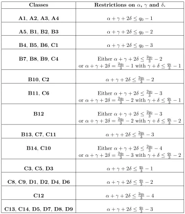
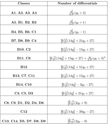
The elements we have produced are all of the formf3g dx, wheregdxcan be any of the 42 forms given by theAi’s,Bi’s,Ci’s andDi’s. Next we introduce certain restrictions on the monomialf =xα_uγ_vδ_{, to make f}3_{gdx a linear combination of elements of the}

basis in Proposition 2.4, then we count the number of such elements in each of the 42 classes. We state these restrictions, for each class, in the following table. (It is taken as read that α≥0 and 0≤γ, δ ≤ q0

3 −1.)

Classes Restrictions on α, γ and δ.

A1,A2,A3,A4 α+γ+ 2δ≤q0−1

A5,B1,B2,B3 α+γ+ 2δ≤q0−2

B4,B5,B6,C1 α+γ+ 2δ≤q0−3

B7,B8,B9,C4 Eitherα+γ+ 2δ ≤ 2q0 3 −2

orα+γ+ 2δ= 2q0

3 −1 with γ+δ ≤

q0 3 −1

B10,C2 α+γ+ 2δ ≤ 2q0 3 −2

B11,C6 Eitherα+γ+ 2δ ≤ 2q0 3 −3

orα+γ+ 2δ= 2q0

3 −2 with γ+δ ≤

q0 3 −1

B12 Eitherα+γ+ 2δ ≤ 2q0 3 −3

orα+γ+ 2δ= 2q0

3 −2 with γ+δ ≤

q0 3 −2

B13,C7,C11 α+γ+ 2δ ≤ 2q0 3 −3

B14,C10 Eitherα+γ+ 2δ ≤ 2q0 3 −4

orα+γ+ 2δ= 2q0

3 −3 with γ+δ ≤

q0 3 −2

C3,C5,D3 α+γ+ 2δ ≤ q0 3 −1

C8,C9,D1,D2,D4,D6 α+γ+ 2δ ≤ q0 3 −2

C12 α+γ+ 2δ ≤ 2q0

3 −4

[image:16.612.74.452.165.603.2]

C13,C14,D5,D7,D8,D9 α+γ+ 2δ ≤ q0 3 −3

Table 2: Restrictions onf.

Classes Number of differentials

A1,A2,A3,A4 q20

2·32(q0+ 3)

A5,B1,B2,B3 q20

2·₃2(q0+ 1)

B4,B5,B6,C1 q20

2·₃2(q0−1)

B7,B8,B9,C4 ₂q30+3·₃4(14q2₀+ 21q0+ 27)

B10,C2 q₂0+33_·34(14q2₀−15q0+ 27)

B11,C6 q0−3

23_·34(14q₀2+ 15q0+ 27) +

q0

2·32(q0+ 3)2

B12 q0−3

23_·34(14q2₀+ 51q0+ 27)

B13,C7,C11 q0−3

23_·34(14q2₀+ 15q0+ 27)

B14,C10 q0−3

23_·34(14q2₀−3q0−27)

C3,C5,D3 q₂0+33_·34(2q2₀+ 21q0+ 27)

C8,C9,D1,D2,D4,D6 q20−9

23_·34(2q0+ 9)

C12 q0−3

23_·34(14q2₀−39q0−27)

C13,C14,D5,D7,D8,D9 q20−9

[image:17.612.90.438.69.466.2]

23_·34(2q0−9)

Table 3: Number of differentials in each class.

Lemma 4.1. Let ω1 = f13g1dx and ω2 = f23g2dx be two holomorphic differentials,

(where fi = xαiuγivδi; αi ≥ 0,0 ≤ γi, δi ≤ q₃0 −1) such that ord∞(ω₁) = ord∞(ω₂). Then

−[ord∞(g₁)−ord∞(g₂)] = 3kq+ 9lq₀+ 3m, (23)

where k, l, m∈Z, with |m|< q0

3 and |l|< 2q0

3 −1.

Proof. Letω1 and ω2 be as above.

ord∞(ω₁) = ord∞(ω₂)

Sincefi =xαiuγivδi,

−ord∞(f_i3) = 3[(αi+γi+ 2δi)q+ 3(γi+δi)q0+δi] ⇒ −ord∞(f₂3)−(−ord∞(f₁3)) = 3[(α₂+γ₂+ 2δ₂)q+ 3(γ₂+δ₂)q₀+δ₂]

−3[(α1+γ1+ 2δ1)q+ 3(γ1+δ1)q0+δ1]

= 3[kq+ 3lq0+m], such thatk, l and m∈Z,

withl andm satisfying the conditions stated above.

Proof. of Theorem 1.2.

Each of the classes Ai, Bi, Ciand Di consists of exact holomorphic differentials ω = f3gdx, for certain monomials f in x, u and v. With the help of Lemma 4.1, it can be verified that no two such differentials have the same orders at P∞, e.g. from B1 and B2we have g1 =x2u+v, with −ord∞(g1) = 3q+ 3q0, and g2 =x2yu+yv, with

−ord∞(g₂) = 4q + 4q₀. Then −ord∞(g₁)−(−ord∞(g₂)) = −q −q₀, which is not of the form 3kq+ 9lq0+ 3m with |m|< q₃0, and|l|< 2₃q0 −1. We can show the same for

each other pair of classes. In particular, all these differentials are different, i.e. there is no overlap between the classes. To count them we add up all the numbers of elements in the 42 classes, as listed individually in the table, giving us a lower bound for the dimension of the space of exact holomorphic differentials. It is precisely

2q0

27 14q

2 0+ 9

+ 1 12 11q

2 0 + 9

,

so we have proved Theorem 1.2.

Conjecture 1.1 is that this lower bound is the exact dimension.

Remark 2: The above sum must obviously be an integer, but we can also see this directly from the formula. Of course 2q0

33 (14q2₀ + 9) is an integer since the numerator

is divisible by 33 (as 3|q0). But also ₃1·4(11q02+ 9)∈Z, since 11q20+ 9≡11×1 + 9 ≡

0 (mod 4), and 11q2₀+ 9 is obviously divisible by 3.

Remark 3: For any large s, comparing the (conjectured) dimension d of the space of exact holomorphic differentials to the genusg= 3₂q0(q−1) shows that it is

approxi-mately a quarter ofg. To be precise, lim s→ ∞

d

g = 24356.

§5 A group action on H0_(X,Ω1₎

yq−y=xq0_(xq_{−x).) Thisθthen also acts naturally as an automorphism of the curve}

X/Fq, and as an Fq-linear transformation ofH0(X,Ω).

θ:

       

      

x7→ζ x y7→ζq0+1_y

u7→ζ3q0+1_u

v7→ζ3q0+3v dx7→ζ dx.

(25)

For eachi(mod(q−1)), let Ai be the subspace of H0(X,Ω1) on whichθ acts as multi-plication byζi. Note that this is independent of the choice ofζ, in fact it is an isotypic component for the action on H0(X,Ω1) of the cyclic group G ≃ F×q generated by θ. Since the order ofGis coprime to the characteristic, we have

H0(X,Ω1) = M i(mod(q−₁₎₎

Ai (26)

The following lemma (suggested by the referee) is immediate.

Lemma 5.1.

xaybucvddx∈ Ai ⇐⇒ a+b(q0+ 1) +c(3q0+ 1) +d(3q0+ 3) + 1≡i (modq−1).

Lemma 5.2. C_{(A3i)⊆ Ai}

Proof. Letω3i ∈ A3i. It follows from the definition in Proposition 3.1 thatCcommutes with automorphisms of the curve. Hence

θC_{(ω3i) =}C_(θω3i)

=C_(ζ3i_ω3i)

=ζiC_(ω3i).

From the above it is clear that C_{(ω3i)∈ Ai, hence} C_{(A3i)⊆ Ai.}

Remark 4: Since 32s+1 _{=q ≡1 (mod(q−1)), C therefore permutes the A}

i in cycles of length dividing 2s+ 1.

Equation (26) and Lemma 5.2 easily imply the following.

Proposition 5.3.

ker(C_{) =} M

i(mod(q−₁₎₎

ker(C_|A

i)

Proposition 5.4.

dim(Ai) =  

 3q0+1

2 if i is odd,

3q0−1

2 if i is even.

Proof. Consider the projection π : X → Y, where Y is the quotient of X by the group G of automorphisms generated by θ. Recall that G is cyclic of order q −1, so π is a morphism of degree q −1. Recall also that yq _{−y = x}q0_(xq _{−x), that}

θ(x) (i.e. the pullback θ∗

(x)) is ζx and θ(y) = ζq0+1_{y. If P = (α, β) ∈ X(}

Fq) with α 6= 0, then θk(P) = (ζkα, ζk(q0+1)β), so the stabiliser of P under the action of G is trivial, and P is not a ramification point for π. At the other extreme, P0 := (0,0)

and P∞ are fixed points for the action of G, with ramification index (q−1). There remain (q−1) points Pβ := (0, β) for β ∈ Fq− {0}. We have θ(Pβ) = Pβζq0 +1. Since

q−1 = (q0+ 1)(3q0−3) + 2, so that g.c.d.(q0+ 1, q−1) = 2, it follows that these points

form two orbits of size (q−1)/2 for the action ofG, and all have ramification index 2. There are four branch points forπ, with inverse images of sizes 1,1,(q−1)/2,(q−1)/2.

Now we are ready to find the genusg(Y) of Y, using Hurwitz’s formula 2g(X)−2 = deg(π)(2g(Y)−2) +P

P∈_X(Fq)(eP−1), for the tamely ramified coverπ :X→Y, where theeP are the ramification indices. Sinceg(X) = 3₂q0(q−1), we get

3q0(q−1)−2 = (q−1)(2g(Y)−2) + 2(q−2) + (q−1) = (q−1)(2g(Y) + 1)−2.

Hence g(Y) = 3q0−1

2 . Since A0 = π

∗

H0(Y,Ω1), this proves the case i = 0 of the proposition.

To prove the other cases, we turn to Lemma 4.3 of Bouw [B], who credits it to Kani [K]. Let Q1 =π(P∞), Q₂ =π(P₀), Q₃ and Q₄ be the branch points of π. The sizes of the inverse images aren1 =n2 =q−1 and n3 =n4 = (q−1)/2. In Bouw’s notation,

ℓ = q −1 and we have numbers bj and aj for 1 ≤ j ≤ 4. Since ordP∞(x) = q, x is a uniformiser at each of the q points Pβ for β ∈ Fq. At P∞, xu/v is a uniformiser, by Proposition 2.1. Sinceθ∗

(x) = ζx while θ∗

(xu/v) =ζ−₁

xu/v (using (25)), we find that b1 =−1 while b2 =b3 =b4 = 1. Now ai is defined to be the multiple of ni such that 0 ≤ ai < ℓ and aibi/ni ≡ 1 (modℓ/ni). It follows that a1 = q−2, a2 = 1 and

a3 =a4 = (q−1)/2.

If we defineLi, for 0≤i < q−1, to be the subspace ofH1(X, OX) on whichθ acts as multiplication byζi, then according to Lemma 4.3 of [B] in our case,

dimLi=g(Y)−1 +

4 X

j=1

iai q−1

,

wherehai is the fractional part ofa. This gives

dimLi=g(Y)−1 +

i(q−2) q−1

+

i q−1

+ 2

i((q−1)/2) q−1

= 3q0−1 2 −1 +

q−1−i q−1 +

i

q−1 + 2hi/2i=

3q0−1

2 + 2hi/2i

=

(_3q 0−1

2 ieven; 3q0+1

2 iodd.

By Serre duality, dimAi = dimLq−1−i, and sinceq−1 is even, the proposition follows.

Remark 5: One may check, using Proposition 2.4 and Lemma 5.1, that the following

3q0+1

2 differentials belong to our basis for H0(X,Ω1) and to A1, so must form a basis

forA1:

dx, x2vq0−1_{dx, x}4_uvq0−2_{dx, ... , x}q0−3_yuq0−2_{vdx, x}q0−1_yuq0−1_dx,

yuq0 −1 2 v

q0−1

2 dx, x2yu q0 +1

2 v q0−3

2 dx, ... , xq0−1uq0−1dx.

§6 Proof of Theorem 1.3

s= 1

TheAi are of size 5 foriodd, 4 for ieven. The following shows, for a few of the Ai’s, a basis (arranged in a lexicographical order).

A1=hdx, yuvdx, x2v2dx, x2yu2dx, x4uvdxi,

A2=hxdx, xyuvdx, x3v2dx, x3yu2dxi,

A3 =hyv2dx, y2u2dx, x2dx, x2yuvdx, x4yu2dxi,

A4 =hxyv2dx, xy2u2dx, x3dx, x3yuvdxi,

A5 =hydx, y2uvdx, x2yv2dx, x2y2u2dx, x4dxi,

A6 =hxydx, xy2uvdx, x3y2u2dx, x5dxi.

These may be confirmed using Proposition 2.4 and Lemma 5.1, but the following in-dicates how these bases were generated in practice. We start with the basis for A1

given by Remark 5. In getting from A1 to A2 we have more-or-less multiplied by x,

but we dropped x5uvdx as it is not holomorphic. To get from A2 to A3, again it is

mostly a case of multiplying byx. We have discarded the non-holomorphicx4_v2_{dx, but}

have gained two by replacingx4 (i.e. xq0+1) withy in both that and the holomorphic x4yu2dx.

As mentioned earlier,C_{maps eachAi toAi/3, and permutes theAi in cycles of length} dividing 2s+ 1. For s= 1, one easily checks that it produces 8 length 3 cycles and 2 length 1 cycles (the latter fori= 0 andi= (q−1)/2). For example

A1

C −→ A9

C −→ A3

Here we show calculations for a part of this cycle,A9

C

−→ A3, where

A9 =huv2dx, y2dx, x2u2vdx, x4ydx, x8dxi

Ifω∈ A9 then we can express ω as

ω=λ3₁(uv2dx) +λ₂3(y2dx) +λ3₃(x2u2vdx) +λ3₄(x4ydx) +λ₅3(x8dx), withλi∈Fq.

Ifω∈ker(C_{)|A9 then}C_{(ω) = 0 shows}

C_{(ω) =}C_(λ3_1(uv2_{dx) +λ}3_2(y2_{dx) +λ3}3_(x2_u2_{vdx) +λ}3_4(x4_{ydx) +λ}3_5(x8_{dx)) = 0}

⇒ λ1C(uv2dx) +λ2C(y2dx) +λ3C(x2u2vdx) +λ4C(x4ydx) +λ5C(x8dx) = 0

⇒ λ1C(uv2dx) +λ2C(y2dx) +λ3C(x2u2vdx) +λ4xC(xydx) +λ5x2C(x2dx) = 0.

(27)

We use Table 1 to substitute into (27). This gives

λ1(x4yu2−x2yuv+yv2)dx+λ2(x2u2vdx) +λ3(x4yu2−x2yuv+yv2)dx+λ4(x2dx)

+λ5(dx) = 0.

Since C(ω) ∈ A3, it can be expressed in terms of the generators of A3. The above

equation becomes

(λ1+λ3)v2ydx+ (0)y2u2dx+ (λ2+λ4+λ5)x2dx+ (−λ1−λ3)x2yuvdx

+ (λ1+λ3)x4yu2dx= 0 (28)

To find ker(C_|A

9), we have to find the null space of the associated matrix M9,3. We

solve the following:



    

1 0 1 0 0 0 0 0 0 0 0 1 0 1 1 2 0 2 0 0 1 0 1 0 0



    



    

λ1

λ2

λ3

λ4

λ5 

    

=



    

0 0 0 0 0



    

.

This gives

λ1=−λ3

λ5=−(λ2+λ4).

From the above we have the following three linearly independent exact holomorphic differentials:

(x2u2v−uv2)dx; (29)

(x4y−y2)dx; (30)

(x8−x4y)dx=x3(x3x2−xy)dx . (31)

For the length-1 cycles, we find that ker(C_{|A13) is spanned by (x}2_{u+v)dx∈B1, while} ker(C_|A

0) is spanned byx

3_(x2_u2_{+uv)dx∈B3and (x}3_uv+xv2_{)dx∈B4. From these}

and similar calculations, we find that the dimension of the space of exact holomorphic differentials H0(X,Ω1)C₌₀

, for s = 1, is 39 (compared with g = 117), and the basis elements we find all lie on the listsAi,Bi,Ci,Di.

s= 2

For s = 2 we can proceed in a similar manner to that described for s = 1, to find, inside eachAi, a subset of our basis for H0(X,Ω1), of size 3q0₂+1 ifiis odd, 3q0

−₁

2 ifiis

even. For example, the following shows our basis (arranged in a lexicographical order) for a few of theAi’s.

A1=hdx, yu4v4dx, x2v8dx, x2yu5v3dx, x4uv7dx, x4yu6v2dx, x6u2v6dx, x6yu7vdx,

x8u3v5dx, x8yu8dx, x10u4v4dx, x12u5v3dx, x14u6v2dx, x16u7vdxi

A2=hxdx, xyu4v4dx, x3v8dx, x3yu5v3dx, x5uv7dx, x5yu6v2dx, x7u2v6dx, x7yu7vdx,

x9u3v5dx, x9yu8dx, x11u4v4dx, x13u5v3dx, x15u6v2dxi

A3 =hyu3v5dx, y2u8dx, x2dx, x2yu4v4dx, x4v8dx, x4yu5v3dx, x6uv7dx, x6yu6v2dx,

x8u2v6dx, x8yu7vdx, x10u3v5dx, x10yu8dx, x12u4v4dx, x14u5v3dxi

A4 =hxyu3v5dx, xy2u8dx, x3dx, x3yu4v4dx, x5v8dx, x5yu5v3dx, x7uv7dx, x7yu6v2dx,

x9u2v6dx, x9yu7vdx, x11u3v5dx, x11yu8dx, x13u4v4dxi

A5 =hyu2v6dx, y2u7vdx, x2yu3v5dx, x2y2u8dx, x4dx, x4yu4v4dx, x6v8dx, x6yu5v3dx,

x8uv7dx, x8yu6v2dx, x10y2v6dx, x10yu7vdx, x12u3v5dx, x12yu8dxi.

We have altogether 242 Ai’s, which give rise to 48 cycles of length 5 and 2 cycles of length 1. We deal with these cycles one by one, just like in the cases= 1, finding each ker(C_|A

i) by solving a set of linear equations. However, the corresponding matrices will

now be either 14×14 or 13×13. We therefore found their null spaces with the help of the computer package Maple. (For the details of these calculations see [F].)

In the case s = 1, we observed that for each cycle of length 3, containing Ai’s all of dimension either 4 or 5, the total contribution of the cycle to dimH0(X,Ω1)C₌0

is precisely dim(Ai). However, in the case s= 2 we found that, for the cycles of length 5, dim(Ai) is only a lower bound for the contribution to dimH0(X,Ω1)C=0of the cycle containing Ai. The length-5 cycles making the smallest contribution (i.e. 13) to the dimension are A40

C −→ A94

C −→ A112

C −→ A118

C −→ A120

C

−→ A40 and A122

C −→ A202

C −→ A148

C − → A130

C −→ A124

C

−→ A122. Looking at the latter in more detail, the contributions

are as follows:

ker(C|A122) is spanned byx

3_v3_{udx∈A4, x}9_u3_{udx∈A4, v}3_{xvdx∈A5andx}6_u3_xvdx∈

A5.

ker(C_|A

202) is spanned byx

ker(C_{|A148) is spanned by x}3_u3_(x3_xu2 _−x2_{uv + v}2_{)dx ∈ B5 and v}3_(x2q0−3_x2_{yv +}

xq0−3_xy2_v+xu2_)dx∈D3.

ker(C|A130) is spanned byx

9_v3_(x2_{u+v)dx∈B1 andu}15_u3_(x2_u+v)dx∈B1.

ker(C_{|A124) is spanned byx}3_v3_(x2_{u+v)dx∈B1, x}9_u3_(x2_{u+v)dx∈B1,andu}3_(x2q0_xy2₋

xq0_x2_{u+xyu)dx∈D1.}

The length-5 cycles making the largest contribution (i.e. 26) to the dimension are A1 −→ AC 81 −C→ A27 −→ AC 9 −→ AC 3 −→ AC 1 and A161 −→ AC 215 −C→ A233 −C→ A239 −C→

A241−C→ A161.

The cycles of length 1 (containingA121 and A242) make smaller contributions:

ker(C_{|A121) is spanned byv}3_(x2_{yu+yv)dx∈B2 and x}6_u3_(x2_{yu+yv)dx∈ B2,while} ker(C_|A

242) is spanned by x

3_v6_(x2_u2 _{+uv)dx ∈ B3, x}9_u3_v3_(x2_u2 _{+ uv)dx ∈ B3,}

x15_u6_(x2_u2 _{+uv)dx ∈ B3, v}6_(x3_{uv +xv}2_{)dx ∈ B4, x}6_u3_v3_(x3_{uv +xv}2_{)dx ∈ B4,}

x12u6(x3uv+xv2)dx∈B4,and x3u6(x3xyu2−x2yuv+yv2)dx∈B6.

All in all, we find that the dimension of the space of exact holomorphic differentials for X, when s = 2, is 837 (compared with g = 3267), which exactly matches with

2q0

33 (14q2₀+ 9) + ₁₂1(11q₀2+ 9), (by putting q0 = 9 andq = 243).

All the exact holomorphic differentials found by our calculations fors= 1 ands= 2 are accounted for by the classesAi,Bi,CiandDi. We checked directly that the numbers found in each class match those given by Table 3. Many of these turn out to be 0 in the cases= 1, and generally speaking, there are many more differentials in the earlier classes than in the later classes.

Now that we have proved Theorems 1.2 and 1.3, we address the question of why we might believe Conjecture 1.1. Originally, we only found the classesAi,Biand Ci, and thought that might be all, so why should we now believe that for everys≥1 the space of exact holomorphic differentials is spanned by those in these classes and theDi, aside from the fact that we can’t find anything else? After finding the classesAi,BiandCi, we then calculated the kernel ofC _{in the case s= 1 and found that, although almost} everything we found was in one of these classes, the differential (x3x2yv+xy2v+xu2)dx, (obtained from A22

C −

→ A16) does not belong to any of them. This is what made us

References

[B] I. I. Bouw, The p-rank of ramified covers of curves, Compositio Math. 126(2001), 295–322.

[CO1] E. C¸ ak¸cak, F. ¨Ozbudak, Subfields of the function field of the Deligne-Lusztig curve of Ree type,Acta Arith. 115(2004), 133–180.

[CO2] E. C¸ ak¸cak, F. ¨Ozbudak, Number of rational places of subfields of the function field of the Deligne-Lusztig curve of Ree type,Acta Arith. 120(2005), 79–106.

[CS] J. H. Conway, N. J. A. Sloane, Sphere Packings, Lattices and Groups, Springer-Verlag, New York, second edition 1993.

[D1] N. Dummigan, The determinants of certain Mordell-Weil lattices,Amer. J. Math.

117(1995), 1409–1429.

[D2] N. Dummigan, Completep-descent for Jacobians of Hermitian curves,Compositio Math.119(1999), 111–132.

[F] S. Farwa,Exact holomorphic differentials on certain algebraic curves. Ph. D. thesis, University of Sheffield, June 2012.

[FGMPW] H. Friedlander, D. Garton, B. Malmskog, R. Pries, C. Weir, Theanumbers of Jacobians of the Suzuki curves, 2011,Proc. Amer. Math. Soc. 141(2013), 3019– 3028.

[G] B. H. Gross, Group representations and lattices, J. Amer. Math. Soc. 3(1990), 929–960.

[H] J. P. Hansen, Deligne-Lusztig varieties and group codes, in Coding theory and algebraic geometry (Luminy, 1991), Lect. Notes Math. 1518, 63–81, Springer-Verlag, 1992.

[HS] J. P. Hansen, H. Stichtenoth, Group codes on certain algebraic curves with many rational points,Appl. Algebra Engrg. Comm. Comput. 1(1990), 67–77.

[K] E. Kani, The Galois module structure of the space of holomorphic differentials of a curve,J. reine Angew. Math. 367(1986), 187–206.

[LO] K.-Z. Li, F. Oort, Moduli of supersingular Abelian varieties, Lect. Notes Math. 1680, Springer-Verlag, 1998.

[P] J. P. Pedersen, A function field related to the Ree group, in Coding theory and algebraic geometry (Luminy, 1991), Lect. Notes Math.1518, 122–131, Springer-Verlag, 1992.

[S] J.-P. Serre, Sur la topologie des vari´et´es alg´ebriques en caract´eristique p, in Inter-national symposium on algebraic topology, 24–53, Universidad National Aut´onoma de Mexico and UNESCO, Mexico City, 1958.