This is a repository copy of SPH study of the evolution of water–water interfaces in dam break flows.
White Rose Research Online URL for this paper: http://eprints.whiterose.ac.uk/86310/
Version: Accepted Version
Article:
Jian, W., Liang, D., Shao, S. et al. (2 more authors) (2015) SPH study of the evolution of water–water interfaces in dam break flows. Natural Hazards. ISSN 0921-030X
https://doi.org/10.1007/s11069-015-1726-6
[email protected] https://eprints.whiterose.ac.uk/
Reuse
Unless indicated otherwise, fulltext items are protected by copyright with all rights reserved. The copyright exception in section 29 of the Copyright, Designs and Patents Act 1988 allows the making of a single copy solely for the purpose of non-commercial research or private study within the limits of fair dealing. The publisher or other rights-holder may allow further reproduction and re-use of this version - refer to the White Rose Research Online record for this item. Where records identify the publisher as the copyright holder, users can verify any specific terms of use on the publisher’s website.
Takedown
If you consider content in White Rose Research Online to be in breach of UK law, please notify us by
1
SPH Study of the Evolution of Water-Water Interfaces in Dam
Break Flows
Wei Jian1, Dongfang Liang2, Songdong Shao3, Ridong Chen4 andXingnian Liu5
1
Department of Engineering, University of Cambridge, Cambridge CB2 1PZ, UK. Email:
2
Department of Engineering, University of Cambridge, Cambridge CB2 1PZ, UK. Email:
3
Department of Civil and Structural Engineering, University of Sheffield, Sheffield S1 3JD,
UK (State Key Laboratory of Hydro-Science and Engineering, Tsinghua University, Beijing
100084, China). Email: [email protected] (Author of Correspondence)
4
State Key Laboratory of Hydraulics and Mountain River Engineering, Sichuan University,
Chengdu 610065, China. Email: [email protected]
5
State Key Laboratory of Hydraulics and Mountain River Engineering, Sichuan University,
2
Abstract
The mixing process of upstream and downstream waters in the dam break flow could
generate significant ecological impact on the downstream reaches and influence the
environmental damages caused by the dam break flood. This is not easily investigated with
the analytical and numerical models based on the grid method due to the large deformation of
free surface and the water-water interface. In this paper, a weakly compressible Smoothed
Particle Hydrodynamics (WCSPH) solver is used to study the advection and mixing process
of the water bodies in two-dimensional dam-break flows over a wet bed. The numerical
results of the mixing dynamics immediately after the release of the dam water are found to
agree satisfactorily with the published experimental and numerical results. Then further
investigations are carried out to study the interface development at the later stage of
dam-break flows in a long channel. The analyses concentrate on the evolution of the interface at
different ratios between the upstream and downstream water depths. The potential
capabilities of the mesh-free SPH modelling approach for predicting the detailed
development of the water-water interfaces are fully demonstrated.
3
1.
Introduction
3
4 5
For free-surface flows, the Smoothed Particle Hydrodynamics (SPH) technique proves to be a 6
promising numerical method in modelling large surface deformations and moving interfaces, 7
even with the presence of water fragmentation and coalescence. Its particle nature provides a 8
straightforward tool for handling complex and moving geometries, since the fluid motion can 9
be easily traced using the Lagrangian description. The SPH method was initially proposed for 10
the astrophysical applications. Lucy (1977) and Gingold and Monaghan (1977) independently 11
modified the Particle-in-Cell (PIC) method to derive a pure particle treatment for the pressure 12
and velocity fields. The particles are linked with each other by a kernel function. Monaghan 13
first extended the SPH application to model incompressible flows with a free surface (1994), 14
in which a weakly compressible assumption was made to model the fluid incompressibility 15
without further computational complication, and an equation of state was used to couple the 16
density and pressure fields. Later studies on the method have extended the application to a 17
variety of hydrodynamic problems. Researches on the surface wave movement, interfacial 18
flow and fluid–structure interaction have demonstrated promising capabilities of the SPH
19
method (e.g. Dalrymple and Rogers, 2006; Violeau and Issa, 2007). In general, it is 20
considered that the SPH method has a great potential for analysing flows involving large 21
deformation, free surface, moving interface, deformable boundary and moving discontinuity. 22
23
Dam-break flows involve the formation of shocks, which arise from the step changes in the 24
initial water level. Under the shallow water assumption, there exist analytical solutions to the 25
problem. However, these may not accurately reflect the actual situations especially in the 26
early stage of the dam break flow, when the large vertical acceleration invalidates the basic 27
foundation of the Shallow Water Equations (SWEs) (Liang, 2010). In recent years, the 28
emphasis of research has shifted to the development of Navier-Stokes (N-S) solvers for the 29
dam-break flows, which have also become a widely used benchmark in the study of the rapid 30
and interfacial flows. Due to its Lagrangian description, the SPH method has been 31
successfully applied to dam-break flows in both two- and three-dimensional configurations. 32
Monaghan (1994) studied a simple dam-break flow to demonstrate the capability of the 33
4
tall structure using a three-dimensional SPH model. The water surface evolutions over dry 35
and wet beds were also analyzed and compared with the experimental data by Crespo (2008) 36
and Crespo et al. (2008). Khayyer and Gotoh (2010) investigated similar problems by using 37
two different mesh-free particle modelling approaches (i.e. MPS/SPH) and evaluated their 38
improved schemes. The major objective of their work is to highlight the potential capabilities 39
of the improved particle numerical schemes in reproducing the detailed features of 40
complicated hydrodynamics. However, their study only focused on the early stage of the dam 41
break flow mixing process and thus the channel length is relatively short. Although very 42
detailed physical mechanisms of dam break flow mixing process have been investigated by 43
Crepso et al. (2008), such as the energy dissipation and vorticity generation, the study is 44
limited by the small spatial and temporal scales of the laboratory test. In addition, Lee et al. 45
(2010) used a three-dimensional WCSPH model to study spillway hydraulics in a practical 46
situation. Furthermore, the two-phase water-sediment mixture interface in a dam break flow 47
was studied by Shakibaeinia and Jin (2011), and water-air interface issue was addressed by 48
Colagrossi and Landrini (2003). More advanced SPH modelling of dam break flows based on 49
the SWEs are attributed to Chang et al. (2011) and Kao and Chang (2012). 50
51
Compared with the pure hydrodynamic studies, the mixing of upstream and downstream 52
waters in dam break flows has been less well understood. The study of dam-break flow 53
mixing process has both theoretical and practical importance in water engineering due to its 54
relevance to the ecological and environmental damages caused by the floods, and the 55
understanding of this process could lead to a better water management and improve the 56
hydro-environmental status of the water system. This paper attempts to numerically model 57
such a mixing process, especially the evolution of the interface between the upstream and 58
downstream waters. As shock waves are always associated with the dam break flows which 59
involve large deformation of free surface and flow interface, the mixing process is a 60
challenge to the traditional analytical and numerical approaches. In this paper, the mesh-free 61
SPH method is applied to the dam-break flow predictions with an emphasis on the associated 62
mixing process. The SPH technique is a mesh-free Lagrangian modelling approach. Its 63
robustness lies in its ability to track the free surfaces and multi-interfaces in an easy and 64
straightforward manner, thus it is well-suited for the study of dam break flow mixing and 65
5
fixed grid system, thus numerical diffusion and complicated mesh re-configurations are 67
unavoidable when treating the multi-interfaces. In addition, by comparing the numerical
68
solutions with the experimental results, the pros and cons of other alternative numerical 69
approaches for predicting such rapidly varied flows are highlighted. 70
71
72
2.
SPH Methodology and Implementation
73
74
75
This section provides a detailed overview of the methodology and implementation of the 76
weakly compressible SPH method, namely the WCSPH method. The SPH formulation is 77
based on the concept of integral interpolations. Using a kernel function to relate the 78
movement of the fluid particles, differential operators in the Navier-Stokes equations can be 79
approximated by summations over the discrete particles. Each particle carries information 80
about the velocity, density, mass, pressure and other flow variables over time (Monaghan, 81
1994). 82
83
In SPH, the approximation of any function f(r) at particle i can be written in terms of the
84
values at neighbouring particles within a compact support zone in the following notation: 85
j
ij j j j
i f W
m
f(r) (r )
(1)
86
where m , j j denote the mass and density of the neighbouring particle j, respectively; r j
87
is the spatial position of the particle j and W represents the kernel function between ij
88
particle i and j, W(ri rj,h), where h is the smoothing length. As in many hydrodynamic
89
computations, the kernel function used here is the Cubic Spline kernel function. It is a third-90
order polynomial with a compact support based on a family of spline functions. The 91
smoothing length is often taken to be h1.0~1.3r, where r is the initial fluid particle
92
spacing. 93
94
The particle approximation for the spatial derivative of a function can be written with regard 95
6
j ij i j j ji f W
m
f(r) (r )
(2)
97
where iWij denotes the gradient of the kernel function with respect to particle i .
98
99
To model incompressible flows, the associated fluid is assumed to be weakly compressible in 100
order to minimise the computational complication. The continuity equation for a weakly 101
compressible fluid takes the following form: 102
v dt
d
(3) 103
where t is the time and v is the velocity vector field. The SPH form of the continuity
104
equation can therefore be derived as: 105
i ijj i j j j i i W m dt
d
v v (4) 106
The momentum equation for a weakly compressible fluid reads: 107
v 1 2vF
P
dt d
(5) 108
where is the viscosity coefficient; P is the pressure and F is the external body force.
109
110
In practice, the pressure gradient is often computed in the following form: 111
j ij i j j i i j i i W P P mP( ) (2) (2 )
r r
r (6)
112
113
Viscosity is important in improving the stability of the simulation. Instead of discretising the 114
viscosity term in Equation (5), the artificial viscosity often used in the WCSPH is proposed 115
by Monaghan (1994) as follows: 116 0 2 ij ij ij ij ij c 0 0 ij ij ij ij r v r v (7) 117
where 2 2
ij ij ij ij h r r v
and the relevant notations can be found in Monaghan (1994). is the
118
bulk viscosity and is the Von Neumann-Richtmyer viscosity. The latter is taken to be zero
119
7
shocks and to avoid the particle interpenetration, but the disadvantage is that it may lead to 121
unphysical decay and diffusion of vorticity in some strong shear flows. Crespo et al. (2008) 122
adopted a value of coefficient = 0.08 for the dam break mixing flows and it was later
123
found by Khayyer and Gotoh (2010) that the simulations could lead to excessive vorticity 124
dissipation. They obtained more stable results when decreasing the coefficient from 0.08 to 125
0.02. By balancing the viscous decay and the integrity of free surface profiles, a value of 0.02 126
was used for all the applications presented in this paper. 127
128
In order to close the equation systems, an equation of state has been adopted to relate the 129
pressure to the density. For water it takes the following form 130 1 0 B
P (8)
131
where 0 is the reference density that is usually set to 1000.0 kg/m3 for water; and is a
132
constant that is normally taken to be 7. The parameter B sets a maximum limit for the density 133
variation allowed in the flow. It is calculated based on c020/ , where c is the speed of 0
134
sound at the reference density. 135
136
The particle positions are updated using the velocity calculated from the momentum equation. 137
In practical computations, the following XSPH variant is used to increase the numerical 138
stability and accuracy 139
j ij ij j j ii m W
dt d v v r
(9)
140
where is a constant in the range between 0.0 and 1.0 depending on the application. In this
141
paper, is taken as 0.5 following Crespo et al. (2008). In most dam break flow simulations,
142
has been taken to be around 0.5 to achieve the best performances (Monaghan, 1994).
143
However, we should realize that the increase of this value may lead to more numerical 144
smoothing effect, so attentions should be paid to calibrate the optimum value for small 145
amplitude waves. 146
8
The time integration procedures of the continuity and momentum equations follow the 148
modified predictor-corrector Euler scheme (Monaghan, 1994). Owing to the large sound 149
speed required for the weakly compressible assumption, very small time step is needed in the 150
WCSPH model to satisfy the CFL condition. In this paper, all of the WCSPH computations 151
are based on an in-house code developed in Liang (2010) and Liang et al. (2010). 152
153
The initial setting of the particle positions plays an important role in the accuracy and 154
computational efficiency of the SPH method. In WCSPH, a common practise is to first 155
conduct a numerical simulation under the hydrostatic condition until the movement of 156
particles becomes very small, and then the actual dynamic simulation starts. On the solid 157
boundaries, the non-penetration condition must be satisfied. In the present work, the 158
Lennards-Jones repulsive force method is used in the WCSPH model for its simplicity and 159
effectiveness. On the free surface, both kinematic and dynamic boundary conditions can be 160
automatically met by the Lagrangian nature of the SPH method. 161
162
It has been noticed that the summation interpolant fails to reproduce a constant function in 163
some actual simulations, which often leads to unphysical variation of the local density field 164
especially near the boundaries. In the WCSPH model used in this work, the Shephard 165
filtering is performed every 40 time steps to reinitialize the density field. Hence, the 166
numerical stability is maintained. One of the major instabilities experienced by the SPH 167
model is the particle clumping in certain simulations. Monaghan (2000) introduced an 168
additional term, f , into the momentum equation to exert a repulsive force between the fluid ij
169
particles with small separations. This force is dependent on the kernel function and the 170
pressure field, which takes the form of 171
n ij j j i i ij r W W P P f 0.01 2 2
(10)
172
where W
r is the kernel function value based on the initial particle spacing; and n is a173
constant normally set at 4. Finally, the momentum equation (5) in SPH form becomes 174
v g
j ij i ij ij j j i i ji m P P f W
dt d
2
2
(11)
175
9
3.
Model Validations: Dam-break Flow Propagation
177
178
179
In this section, the propagation of a dam-break flow is simulated and validated against the 180
experimental work detailed in Stansby et al. (1998), the analytical solutions to the Shallow 181
Water Equations and the numerical solutions to the Navier-Stokes equations using the 182
Volume of Fluid (VOF) method (Jian, 2013), in which FLUENT13.0 is used and thus the 183
numerical scheme is based on the Finite Volume method. The test case considers the
184
instantaneous collapse of a dam in a wide, horizontal and frictionless channel of 200 m long. 185
Water is initially static and separated by a gate located at x = 100 m. The initial conditions are 186 defined as: 187
m 100 if m 100 f 0 , , 0 0 , 0 1 x h x h x h xu i (12)
188
where h is the initial water depth upstream of the dam; and 0 h1 is the initial water depth in
189
the downstream channel. In this study, the upstream water depth h is kept constant at 10.0 m, 0
190
while three different values have been considered for h1: 0.0 m for a dry bed, 1.0 m for a
191
shallow wet bed, and 4.5 m for a deep wet bed, respectively. 192
193
The parameters used in the WCSPH model are: initial particle spacing r = 0.1 m and time
194
step t = 0.0002 s. In the grid-based VOF model, the main computational parameters are:
195
grid size of 0.1 × 0.1 m2 and time step t = 0.005 s. Hence, the spatial resolutions of the
196
mesh-free and grid-based models are comparable. 197
198
3.1 Results and discussions
199
200
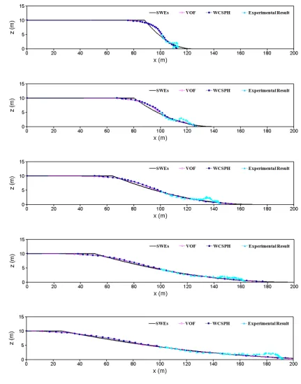
Figures 1 to 3 illustrate the comparisons among the numerical results of the WCSPH model, 201
the experimental data of Stansby et al. (2008), analytical solutions to the SWEs (Jian, 2013) 202
and numerical solutions to the Navier-Stokes equations using the VOF method (Jian, 2013), 203
with the initial downstream water depths being h1 = 0.0 m, 1.0 m and 4.5 m, respectively.
204
205
10 207
208 209
210 211
212 213
214 215
[image:11.595.78.510.119.669.2]216 217 218
Figure 1 Free surface profiles in the dam-break flow over dry bed h1 = 0.0 m, at t = 1.20 s, 219
2.00 s, 3.60 s, 5.00 s and 7.40 s, respectively 220
11 223
224 225
226 227
228 229
[image:12.595.73.509.116.564.2]230 231 232
Figure 2 Free surface profiles in the dam-break flow over shallow wet bed h1 = 1.0 m, at t = 233
2.40 s, 4.00 s, 6.60 s and 9.00 s, respectively 234
235
236
237 238
239
240
241
12 243
244
245 246
247 248
249 250
[image:13.595.83.509.145.573.2]251 252
Figure 3 Free surface profiles in the dam-break flow over deep wet bed h1 = 4.5 m, at t = 253
2.00 s, 3.00 s, 5.20 s and 7.60 s, respectively 254
255
256
257
258
13
It is seen from Figures 1 to 3 that the flow caused by the collapsed dam behaves very 260
differently depending on the downstream depths. For a dry bed, the forward momentum 261
dominates the fluid movement and the flood front is established very quickly. Figure 1 shows 262
that, by t = 1.20 s, the wave front has already settled into a stable form and its propagation
263
for the rest of simulation is free of any breaking. If there is initially a layer of water in the 264
downstream channel, the upstream water can build up into the front with a significant height. 265
A mushroom-like waveform emerges in both Figures 2 and 3 immediately after the dam 266
collapses. The downstream condition generally determines the shape of the wave front that 267
propagates downstream. If the initial downstream water depth is shallow, the accumulated 268
water front soon breaks onto the static water in the channel, driven by the large pressure 269
gradient as shown in the surface profile at t = 6.60 s in Figure 2. The broken wave front
270
continues to travel downstream, accompanied by some small-scale breakings at the interface 271
between the reservoir water and the channel water. The overall waveform under the shallow 272
water layer condition is characterised by the water front travelling downstream. This is, 273
however, not the case in the deep downstream water condition as shown in Figure 3, in which 274
the mushroom-like water front seen at t = 2.00 s gradually evolves into two distinct wave
275
forms travelling in the opposite direction. The experimental data suggests that the 276
downstream-propagating water front is slightly more prominent, whereas the numerical 277
results indicate a more balanced strength between the two wave fronts. 278
279
All of the three scenarios observe a good agreement between the WCSPH and VOF 280
computations against the experimental data. Both models are based on the Navier-Stokes 281
equations and are able to predict the propagation of the dam-break flow with good accuracy. 282
However, slight discrepancies exist in the propagation speed between the experimental 283
observations and numerical predictions. Due to the assumption of frictionless solid 284
boundaries, the propagation of the wave front is over-predicted under the dry bed condition. 285
In addition, the numerical predictions tend to estimate a more rapid wave front development 286
under the deep downstream water layer setting. For all three cases, the solutions to the SWEs 287
deviate significantly from the experimental observations immediately after the dam collapse. 288
This is because the SWEs are only able to provide approximate predictions of the free surface 289
when there is insignificant variation in the vertical direction (Liang, 2010). Therefore, some 290
14
Despite this, the propagation speed of the wave front agrees well with the experimental data, 292
except that a slight over-estimation is found for the case of the deep ambient layer. Once the 293
flow has settled into an established form at the later stage, the accuracy of the SWEs 294
prediction improves significantly as the flow characteristics satisfy the underlying long-wave 295
assumptions adopted in deriving the SWEs. Similar observations have also been reported in 296
Pu et al. (2013). 297
298
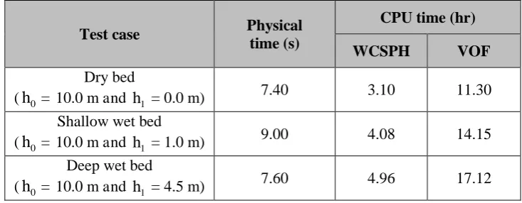
One distinct advantage of the WCSPH model is its superior computational efficiency over the 299
VOF model for the three cases considered here. Table 1 lists the CPU time required for 300
simulating the cases using the WCSPH and VOF models. Since the VOF method needs to 301
simulate the flow of both the water and air phases, it requires a significantly longer 302
computational time. 303
[image:15.595.113.480.415.558.2]304
Table 1 CPU time required for the dam-break flow simulations
305
306
Test case Physical
time (s)
CPU time (hr)
WCSPH VOF
Dry bed
(h0 = 10.0 m and h1 = 0.0 m)
7.40 3.10 11.30
Shallow wet bed (h0 = 10.0 m and h1 = 1.0 m)
9.00 4.08 14.15
Deep wet bed
(h0 = 10.0 m and h1 = 4.5 m) 7.60 4.96 17.12
307
308
309
4.
Model Application: Mixing Process in Near-field Dam-break Flows
310
311 312
From the model validations in the previous section, we understand that, in the case of a wet 313
downstream bed, the collapsed water undergoes a dynamic interaction with the water body 314
downstream, which incurs significant mechanical energy dissipation. This section pays 315
15
molecular diffusion, the mixing of the water bodies can be considered as the non-uniform 317
advection of the water associated with the violent wave movements. Here, we apply the 318
WCSPH model to focus on the mixing process involved in the early stage of dam-break flows. 319
The numerical results are compared with the published experimental results. We need to 320
mention that no advanced turbulence closures are included in the WCSPH model, except the 321
artificial viscosity mentioned before. The term of near-field indicates the mixing process 322
situation immediately after the dam break when the interface between the reservoir water and 323
tail water is very complicated. 324
325
4.1 Model setup and computational parameters
326
327
The validation case examines the interaction between two water bodies in a dam-break flow 328
problem immediately after the release of the dammed water. The numerical study is based on 329
the experiment in Janosi et al. (2004). Figure 4 shows the experimental setup of a two-330
dimensional flume with two compartments separated by a gate at x = 0.38 m. A volume of 331
water with a height of 0.15 m (h ) is initially locked up in the upstream compartment. The 0
332
gate is gradually lifted up at a removal rate of approximately 1.5 m/s after the experiment 333
starts, allowing the initially locked water to seep through the opening. Several different 334
downstream depths are considered: shallow ambient layer with depth h1 = 0.015 m and deep
335
ambient layer with h1 = 0.030 m, 0.058 m and 0.070 m, respectively.
336
337
338 339
Figure 4 Experimental setup of the dam-break flow in Janosi et al. (2004)
340
341
To increase computational efficiency, a shorter computational domain was adopted in the 342
16
length can be reduced to 2.5 m without affecting the results. In the SPH computations, the 344
initial particle spacing is r = 0.001 m in the shallow depth condition and 0.002 m in the
345
deep depth condition. The corresponding time steps are t = 1.0×10⁻⁵ s and 2.0×10⁻⁵ s,
346
respectively. The gate is modelled by a set of repulsive particles, with their positions and 347
velocities externally specified to resemble the removal procedure. The two water bodies are 348
tracked by assigning different flags to the upstream and downstream water particles at the 349
beginning of the simulation so that the mixing interface can be identified as the separation of 350
the particles carrying different flags. 351
352
4.2 Results and discussions for the shallow ambient layer
353
354
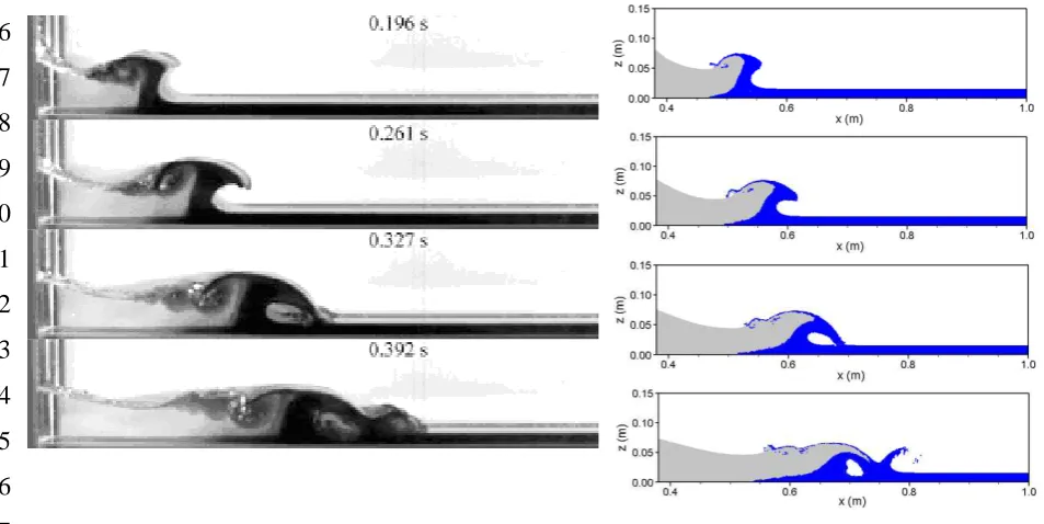
The WCSPH results and the experimental observations (Janosi et al., 2004) are compared in 355
Figure 5 for the case of the shallow ambient layer depth h1 = 0.015 m. It is evident that the
356
numerical model is able to reproduce the wave propagation after the gradual removal of the 357
gate. The main features observed in the experimental snapshots, such as the formation of a 358
mushroom-like water jet and the subsequent wave breakings, are resembled in the numerical 359
predictions with reasonable accuracy. There are some discrepancies in the mixing profiles 360
between the experimental and numerical results. The mixing interface observed during the 361
experiment remains relatively vertical throughout the time with only a slight sloping towards 362
the downstream direction at t = 0.392 s. In addition, the profiles at t = 0.327 s and 0.392 s
363
suggest that the plunging wave front is mostly composed of channel water. The numerically 364
predicted interfaces exhibit varying degrees of inclination towards the downstream in their 365
mixing profiles. However, the overall agreement is still satisfactory. 366
367
Another key feature observed in the mixing patterns is the presence of a thin layer of 368
downstream water at the surface upstream of the plunging water front. That water is brought 369
to the surface by an up-thrust movement during the initial collision of the two water bodies. 370
The WCSPH model is able to capture the presence and development of this thin water layer. 371
372
373
374
17 376
377
378
379
380
381
382
383
384
385
386
[image:18.595.49.526.97.336.2]387
Figure 5 Experimental (left, Janosi et al., 2004) and numerical (right) mixing patterns at
388
t = 0.196 s, 0.261 s, 0.327 s and 0.392 s for shallow flow depth h1 = 0.015 m
389
390
4.3 Results and discussions for the deep ambient layers
391
392
Three large downstream flow depths have been analysed, i.e. h1 = 0.030 m, 0.058 m and
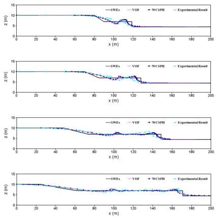
393
0.070 m. Figure 6 presents the experimental snapshots and numerical predictions of the 394
mixing patterns at t = 0.30 s. It is shown that with the increased downstream water depth, the
395
collision between the two water bodies and the subsequent breaking exhibit quite different 396
characteristics from those shown in the shallow ambient layer condition. 397
398
With h1 = 0.030 m, the wave front shows an established mushroom-like shape at t = 0.30 s.
399
The formation of the waveform is slower when compared with the case in Figure 5 for the 400
shallow layer. Generally speaking, the SPH simulations show a satisfactory agreement with 401
the experimental results at t = 0.30 s. The discrepancy lies in the amount of downstream
402
water at the surface. The experimental snapshot suggests that the downstream water makes up 403
approximately half of the plunging wave column, whereas the numerical prediction only 404
shows a relatively thin layer at the free surface which is similar to the case of the shallow 405
ambient layer. Figure 6 also shows that the waveforms take longer time to fully develop with 406
increasing downstream water depth. The experimental snapshots for h1 = 0.058 m and 0.070
18
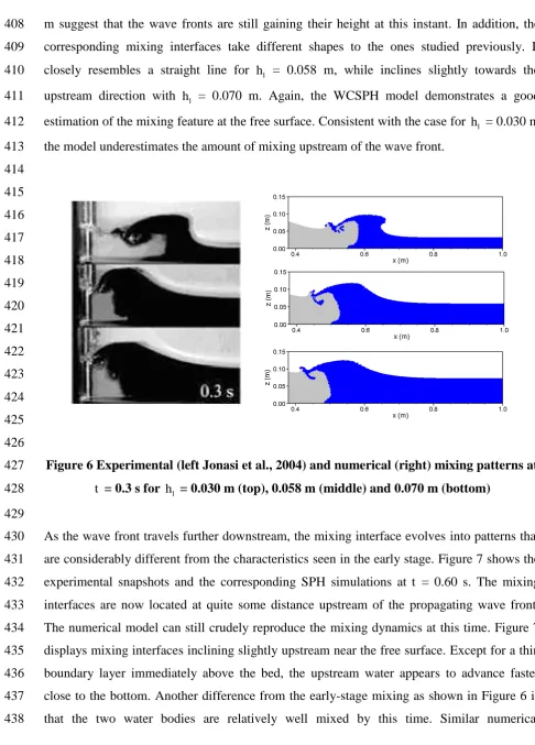
m suggest that the wave fronts are still gaining their height at this instant. In addition, the 408
corresponding mixing interfaces take different shapes to the ones studied previously. It 409
closely resembles a straight line for h1 = 0.058 m, while inclines slightly towards the
410
upstream direction with h1 = 0.070 m. Again, the WCSPH model demonstrates a good
411
estimation of the mixing feature at the free surface. Consistent with the case for h1 = 0.030 m,
412
the model underestimates the amount of mixing upstream of the wave front. 413
414
415
416
417
418
419
420
421
422
423
424
425
[image:19.595.32.519.90.768.2]426
Figure 6 Experimental (left Jonasi et al., 2004) and numerical (right) mixing patterns at
427
t = 0.3 s for h1 = 0.030 m (top), 0.058 m (middle) and 0.070 m (bottom)
428
429
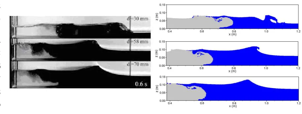
As the wave front travels further downstream, the mixing interface evolves into patterns that 430
are considerably different from the characteristics seen in the early stage. Figure 7 shows the 431
experimental snapshots and the corresponding SPH simulations at t = 0.60 s. The mixing
432
interfaces are now located at quite some distance upstream of the propagating wave front. 433
The numerical model can still crudely reproduce the mixing dynamics at this time. Figure 7 434
displays mixing interfaces inclining slightly upstream near the free surface. Except for a thin 435
boundary layer immediately above the bed, the upstream water appears to advance faster 436
close to the bottom. Another difference from the early-stage mixing as shown in Figure 6 is 437
19
simulations have also been carried out using the VOF method (Jian and Liang, 2012), which 439
found that the WCSPH model is computationally more efficient than the VOF model for all 440
the depths considered. 441
442
443
444
445
446
447
448
449
[image:20.595.53.554.164.353.2]450
Figure 7 Experimental (left Jonasi et al., 2004) and numerical (right) mixing patterns at
451
t = 0.6 s for h1 = 0.030 m (top), 0.058 m (middle) and 0.070 m (bottom)
452
453
454
5.
Model Application: Dam Break Flow Mixing in a Long Channel
455
456
In this section, the WCSPH model is applied to study the interface development of dam break 457
flow in a long channel. We will focus on the later stage of the mixing process, when the 458
interface becomes less chaotic. Immediately after the dam-break, there is a violent mixing 459
between the reservoir water and tail water due to the formation of the vortices. The later stage 460
is when these violent vortical motions settle down after the flood front has travelled some 461
distance downstream. At this stage, the interface between different water regions is quite 462
clear, and can be approximated by using a straight line. The study would be useful for
463
evaluating the hydro-environment in long waterways. The bores in the waterways can be 464
formed by not only the dam breaks but also tides and tsunamis. 465
466
467
5.1 Model setup and computational parameters
468
20
The numerical setup of this hypothetical dam-break problem consists of a 2000 m long 470
horizontal water tank. Water is initially stagnant and separated by a gate located at x= 1000
471
m. The initial conditions are thus defined as: 472
m 1000 if m 1000 f 0 , , 0 0 , 0 1 x h x h x h xu i (13)
473
The initial upstream water depth h is set at 10.0 m throughout the study. Several 0
474
downstream water depths have been investigated, ranging from 2.0 m ~ 7.0 m. As a reference, 475
the analytical solution to the SWEs (Jian, 2013) is included to evaluate the predictions of dam 476
break wave propagations and the corresponding mixing process. 477
478
In the WCSPH model, a particle size of 0.2 m is used for the best compromise between the 479
computational efficiency and accuracy. The total simulation time is 50.0 s, which ensures that 480
the wave front even under the smallest depth ratio does not reach the downstream end of the 481
channel. The computational time step is t = 0.0004 s.
482
483
5.2 Discussion on the flow field
484 485
The numerical results of the WCSPH model are compared with the analytical solutions to the 486
SWEs. It has been well known that the SWEs model is capable of producing reasonable 487
estimations of the wave propagation at the later stage of dam-break flows when there is less 488
variation in the vertical direction. Three downstream water depths (h1) are considered for the
489
validation purpose: h1 = 2.00 m, 5.00 m and 7.00 m. The simulations aim to test the shallow
490
water assumptions and provide a full picture of the wave propagations over the shallow, 491
medium and deep water depths. 492
493
For the smallest downstream water depth h1 = 2.00 m, the WCSPH results agree extremely
494
well with the solutions to the SWEs in terms of the surface profiles as shown in Figure 8. 495
However, when the downstream water depths increase to h1 = 5.0 m and 7.0 m, the wave
496
propagations predicted by the WCSPH model in Figures 9 and 10 fall behind the analytical 497
predictions according to the SWEs. It is also shown that this difference in the propagation 498
speed increases with time and the downstream water depth. 499
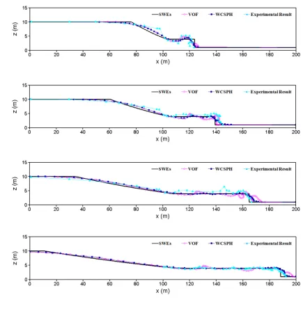
21 501
502
503 504
505 506
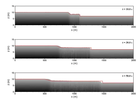
Figure 8 Analytical solutions (solid line) and WCSPH results (shaded area) of surface
507
profiles at t = 10.0 s, 30.0 s and 50.0 s for h = 10.0 m and 0 h1 = 2.0 m
508
509
510 511
22 514
515
Figure 9 Analytical solutions (solid line) and WCSPH results (shaded area) of surface
516
profiles at t = 10.0 s, 30.0 s and 50.0 s for h = 10.0 m and 0 h1 = 5.0 m
517
518
519
520 521
522 523
[image:23.595.67.511.287.622.2]524 525
Figure 10 Analytical solutions (solid line) and WCSPH results (shaded area) of surface
526
profiles at t = 10.0 s, 30.0 s and 50.0 s for h = 10.0 m and 0 h1 = 7.0 m
527
528
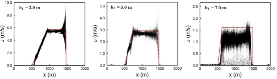
The situations in Figures 8 to 10 are consistent with the horizontal velocity distributions of 529
the three downstream flow depths computed at t = 50.0 s, as shown in Figure 11. The
530
average velocity predicted by the WCSPH model agrees well with the SWEs prediction at h1
23
= 2.0 m, but is 3.3% smaller at h1 = 5.0 m and 25% smaller at h1 = 7.0 m. The discrepancy is
532
thought to be caused mainly by the over-estimation of fluid bulk speed arisen from the 533
uniform velocity distribution over the depth in the SWEs. In the previous validation case, the 534
solutions to the SWEs also tend to give a faster propagation at the deep downstream water 535
layer when compared with experimental observations. The VOF modelling results in Jian 536
(2013) also confirms the accuracy of the present WCSPH computations. 537
538
[image:24.595.76.521.266.393.2]539 540
Figure 11 Analytical solutions (solid line) and WCSPH results (dot) of the velocity
541
distribution at t = 50.0 s for h1 = 2.0 m, 5.0 m and 7.0 m
542
543
Here we need to point out that Figures 8 to 10 show some kinds of oscillations around the 544
wave front in the SPH results while these are not found in the analytic solutions of SWEs. 545
Due to the assumption of hydrostatic pressure distribution in the SWEs, the SWEs model 546
always generates a step wave front without numerical dispersion. The refinement of the 547
SWEs by adding the Boussinesq terms could demonstrate much more satisfactory 548
performance in the case of rapidly varied flows such as dam break in an open channel, which 549
was reported in the latest SPH applications in the field (Chang et al., 2014). 550
551
5.3 Discussion on the mixing
552
553
Disregarding the chemical reaction and molecular diffusion between the upstream and 554
downstream waters, the mixing interface can be determined solely by the advection of fluid 555
particles. Here, the evolution of mixing dynamics is analysed with regard to the interface 556
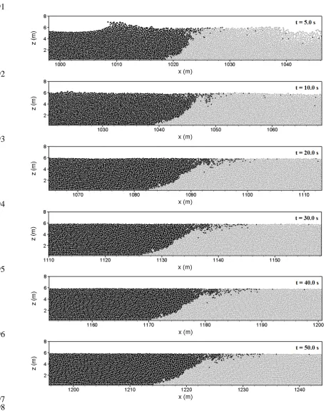
24 558
Figure 12 presents the mixing profiles from t = 5.0 s to 50.0 s for the downstream depth h1 =
559
3.0 m and the corresponding horizontal velocity profiles are shown in Figure 13 (sloped lines 560
in the velocity figures indicate the location of interface between the reservoir water and tail 561
water). The early surface profiles indicate that the waveforms have already settled into some 562
well-established propagating fronts, with little wave breaking across the flow field. The 563
velocity profile at t = 0.0004 s shows a large gradient in the horizontal velocity field along
564
the initial discontinuity. This reflects the large momentum exerted by the collapsed water on 565
the stagnant downstream flow. The velocity gradient causes the vertically positioned interface 566
to slowly evolve into an inclined slope. By the time t = 5.0 s, the surface profile indicates
567
that the interface has already developed into a curve with a larger steepness near the free 568
surface. The velocity profile at t = 5.0 s still exhibits a large velocity gradient over the depth.
569
The magnitude within the immediate mixing zone is approximately less than 4.0 m/s at the 570
lower part of the water depth and over 4.5 m/s at the upper part. This drives the mixing 571
interface to incline further downstream. By t = 10.0 s, the interface becomes more inclined,
572
mainly driven by the fast-moving fluid particles above the mid-depth. The velocity gradient 573
has reduced by at least 0.3 m/s across the depth in the mixing zone that envelops the interface. 574
From t = 10.0 s to 20.0 s, the velocity gradient within the mixing zone has further reduced by
575
approximately 0.2 m/s. Most of the fast-moving particles seen at t = 10.0 s have slowed
576
down. Only a small number of them are still visible within 1.0 m beneath the free surface in 577
the velocity profile at t = 20.0 s. Beyond t = 20.0 s, the mixing interface seems to settle into
578
a relatively stable shape. Little change is observed in the mixing interface from t = 20.0 s to
579
50.0 s. The slope of the interface is approximately 32° above the mid-depth while the lower 580
part remains at around 20°. The velocity fields indicate that the flow domain has settled at a 581
horizontal velocity of around 4.4 m/s for the rest of the simulation. 582
583
584
585
586
25 591
592
593
594
595
596
[image:26.595.47.505.102.680.2]597 598
Figure 12 Mixing patterns for downstream water depth h1 = 3.0 m at t = 5.0 s, 10.0 s,
599
20.0 s, 30.0 s, 40.0 s and 50.0 s
600
26 602
603
604
605
606
607
608 609
Figure 13 Horizontal velocity distributions for downstream water depth h1 = 3.0 m at t
610
= 0.0004 s, 5.0 s, 10.0 s, 20.0 s, 30.0 s, 40.0 s and 50.0 s
27
Similar features of the interface evolution and velocity distribution can also be observed at a 612
larger downstream water depth h1 = 6.0 m. Owing to the larger pressure force and inertia
613
effect of the downstream water body, the interfaces are much steeper than the small depth 614
case at all instants. However, the mixing process still settles into a stable state within the 615
immediate mixing zone by t = 20.0 s. The horizontal velocity settles at an equilibrium value
616
of approximately 2.1 m/s beyond t = 20.0 s. There is little change to the interfacial curves
617
after this time. The detailed results are not plotted in this paper to save space, but interested 618
readers are referred to Jian (2013). 619
620
In summary, the interfaces all take the shape of a forward-leaning line a certain period after 621
the initiation of the dam-break. The mixing interface developments for a range of 622
downstream water depths, varying from h1 = 2.0 m to 7.0 m, are tracked over the time and
623
plotted in Figure 14. The x-axis shows the span of the mixing curve from its most upstream 624
point near the bottom of the channel to its most downstream point at the free surface. In order 625
to minimise the complication at the bottom boundary, the interfaces are tracked from a 626
distance equivalent to one particle size above the solid boundary. Figure 14 shows the 627
evidence that the equilibrium state is reached by t = 20.0 s for most of the depth ratios. Very
628
little change in the interface shapes takes place after this time, except for h1 = 7.0 m, where
629
small adjustments can be found at the later time. All interfaces at t = 10.0 s demonstrate a
630
change in the slope of the interface above the mid-depth. The lower part of the interfaces 631
undergoes only slight adjustment in the process of reaching their equilibrium forms, 632
especially for h1 > 5.0 m. Most of the changes occur near the free surface, where fluid
633
particles take longer time to slow down. The horizontal span of the mixing interface 634
decreases with the increasing depth ratio (h1/ h0), and a larger h1/ h0 also corresponds to the
635
faster establishment of the final equilibrium state. These can be explained by the influence of 636
the horizontal velocity gradient in the vertical direction, since a larger downstream water 637
depth gives rise to smaller velocity non-uniformity over the water column. Generally 638
speaking, the mixing dynamics are significantly affected by the horizontal velocity gradient 639
over the water depth. There are no further changes in the interface curve when the 640
equilibrium state is reached in the horizontal velocity field. 641
28 643
644
645
[image:29.595.81.495.315.473.2]646 647
Figure 14 Mixing interface developments for h1 = 2.0 m ~ 7.0 m
648
649
29
5.4 Fully established mixing interface and its dependence on the depth ratio
651
652
The discussions in the previous section suggest that the initial depth ratio plays an important 653
role in the mixing dynamics in dam-break flows. This section further studies the effect of the 654
initial depth ratios on the final mixing interface at the equilibrium state. Figure 15 shows the 655
mixing profiles at t = 50.0 s for different downstream water depth ratios (h1/ h0). It is
656
evident that the slope of the mixing interface at the equilibrium state is positively correlated 657
to the initial ratio between the downstream and upstream water depths. As discussed earlier, 658
the final forms of the interface are generally determined by the horizontal velocity 659
distributions in the first 20 seconds of the simulation. Figure 16 details the velocity fields of 660
the mixing zone containing the interface for different depth ratios at t = 10.0 s.
661
Reading from the scales of the velocity fields as indicated in the legends, it is evident that the 662
magnitude of the velocity gradient decreases with the increasing depth ratio. As a result, the 663
interface reaches the equilibrium state much faster and the slope of the corresponding 664
interface profile is also expected to be steeper for the deep downstream water depth. 665
666
[image:30.595.156.417.467.677.2]667
Figure 15 Mixing interface profiles for different depth ratios at t = 50.0 s
668
30 670
671 672
673 674
675 676
677 678
679 680
[image:31.595.62.505.109.712.2]681 682 683
Figure 16 Horizontal velocity profiles for different depth ratios at t = 10.0 s
31 685
Each of the mixing interface profile in final steady state in Figure 15 can be normalised using 686
the water depth of the mixing zone in the vertical direction and using the span of the interface 687
in the horizontal direction. The normalized curves are plotted in Figure 17, which shows 688
consistently similar forms regardless of the initial depth ratios. The overall angle of the slopes 689
is approximately 45°. There exists a slight change of the slope at 20% of the water depth 690
below the water surface. The slope of the interface becomes milder above this height. 691
[image:32.595.150.423.278.523.2]692 693
Figure 17 Normalized mixing interface curves for different depth ratios in equilibrium
694 695 696
697
6.
Conclusions
698
699
700
This paper reports on the mixing process involved in both early and later stages of the dam-701
break flows, using the WCSPH simulations and the analytical solutions to the SWEs. A case 702
study concerning dam-break flow propagation is first carried out to validate the WCSPH 703
32
conditions. The results from the model agree well with the experimental measurements, 705
analytical solutions to the SWEs and numerical predictions based on the VOF model. Then 706
the mixing process involved in dam-break flows is examined for the period immediately after 707
the gate opening. The performance of the WCSPH model is validated against the 708
experimental results for the near-field dam-break problem, proving its ability of simulating 709
the mixing dynamics with satisfactory accuracy for both the shallow and deep ambient water 710
layers. 711
712
The subsequent application pays attention to the mixing dynamics and the water-water 713
interface development at the later stage of dam-break flow in a long water tank of 2000 m. 714
Six different water depth ratios have been considered in the study. The SWEs tend to predict 715
a faster propagation of the interface, particularly for the larger depth ratios, but they agree 716
well with the WCSPH simulations in the shallow downstream water condition. The numerical 717
results of the WCSPH model show that for all the depth ratios considered, the equilibrium 718
state is reached by approximately t = 20.0 s after the instantaneous release. The interface
719
curvature and velocity gradient remain largely unchanged afterwards. The numerical 720
outcomes suggest that the interface develops into a curved slope soon after the simulation 721
starts, driven by the gradient in the horizontal velocity field over the depth. As time elapses, 722
the interface becomes more gradual near the surface as the fluid particles in the mid-depth 723
region slow down more rapidly than the ones at the water surface. The slope of the mixing 724
interface at the equilibrium state becomes steeper with the increasing downstream water 725
depth. 726
727
As for the future research direction, it is recognised that the three-dimensional model is 728
necessary to be able to reproduce a more realistic mixing process in dam break flows in a 729
narrow channel where the side-wall effect is strong and the bed topography is complex. 730
731
732
Acknowledgements
733
734
The first author acknowledges the Jafar Studentship during her PhD study at the University of 735
Cambridge. The other authors acknowledge the support of the
33
Major State Basic Research Development Program (973) of China (No. 2013CB036402), 737
Open Fund of the State Key Laboratory of Hydraulics and Mountain River Engineering, 738
Sichuan University (SKHL1404; SKHL1409), Start-up Grant for the Young Teachers of 739
Sichuan University (2014SCU11056) and National Science and Technology Support Plan 740
(2012BAB0513B0). 741
742
743
744
References
745
746
Chang, T. J., Chang, K. H. and Kao, H. M. (2014), A new approach to model weakly 747
nonhydrostatic shallow water flows in open channels with smoothed particle hydrodynamics, 748
Journal of Hydrology, 519, 1010-1019. 749
750
Chang, T. J., Kao, H. M. and Chang, K. H. (2011), Numerical simulation of shallow-water 751
dam break flows in open channels using smoothed particle hydrodynamics, Journal of 752
Hydrology, 408, 78-90. 753
754
Colagrossi, A. and Landrini, M. (2003), Numerical simulation of interfacial flows by 755
smoothed particle hydrodynamics, Journal of Computational Physics, 191(2), 448-475. 756
757
Crespo, A. J. C. (2008), Application of the Smoothed Particle Hydrodynamics Model 758
SPHysics to Free-surface Hydrodynamics, Ph.D. thesis, Universidade de Vigo. 759
760
Crespo, A. J. C., Gómez-Gesteira, M. and Dalrymple, R. A. (2008), Modelling dam break 761
behaviour over a wet bed by a SPH technique, Journal of Waterway, Port, Coastal and Ocean 762
Engineering, 134(6), 313-320. 763
764
Dalrymple, R. A. and Rogers, B. D. (2006), Numerical modelling of water waves with the 765
SPH method, Coastal Engineering, 53(2-3), 141-147. 766
34
Gingold, R. A. and Monaghan, J. J. (1977), Smoothed particle hydrodynamics: theory and 768
application to non-spherical stars, Royal Astronomical Society Monthly Notices, 181, 375-769
389. 770
771
Gómez-Gesteira, M. and Dalrymple, R. A. (2004), Using a 3D SPH method for wave impact 772
on a tall structure, Journal of Waterway, Port, Coastal and Ocean Engineering, 130(2), 63-69. 773
774
Jánosi, I. M., Jan, D., Szabó, K. G. and Tél, T. (2004), Turbulent drag reduction in dam-break 775
flows, Experiments in Fluids, 37, 219-229. 776
777
Jian, W. (2013), Smoothed Particle Hydrodynamics Modelling of Dam-break Flows and 778
Wave-structure Interactions, Ph.D. thesis, The University of Cambridge. 779
780
Jian, W. and Liang, D. (2012), On simulating mixing process in dam-break flows, 781
Proceedings of 2nd IAHR Europe Conference, Munich, 27-29 June, 1-6.
782
783
Kao, H. M. and Chang, T. J. (2012), Numerical modeling of dambreak-induced flood and 784
inundation using smoothed particle hydrodynamics, Journal of Hydrology, 448, 232-244. 785
786
Khayyer, A. and Gotoh, H. (2010), On particle-based simulation of a dam break over a wet 787
bed, Journal of Hydraulic Research, 48(2), 238-249. 788
789
Lee, E.-S., Violeau, D., Issa, R. and Ploix, S. (2010), Application of weakly compressible and 790
truly incompressible SPH to 3-D water collapse in waterworks, Journal of Hydraulic 791
Research, 48(Extra Issue), 50-60. 792
793
Liang, D. (2010), Evaluating shallow water assumptions in dam-break flows, Proceedings of 794
the ICE – Water Management, 163(5), 227-237.
795
796
Liang, D., Thusyanthan, I., Madabhushi, S. P. G. and Tang, H. (2010), Modelling solitary 797
waves and its impact on coastal houses with SPH method, China Ocean Engineering, 798
35 800
Lucy, L. (1977), A numerical approach to the testing of fission hypothesis, The Astronomical 801
Journal, 82(12), 1013–1024.
802
803
Monaghan, J. J. (1994), Simulating free surface flows with SPH, Journal of Computational 804
Physics, 110, 399-406. 805
806
Monaghan, J. J. (2000), SPH without a tensile instability, Journal of Computational Physics, 807
159(2), 290-311. 808
809
Pu, J., Shao, S., Huang, Y. and Hussain, K. (2013), Evaluations of SWEs and SPH numerical 810
modelling techniques for dam break flows, Engineering Applications of Computational Fluid 811
Mechanics, 7(4), 544-563. 812
813
Shakibaeinia, A. and Jin, Y. C. (2011), A mesh-free particle model for simulation of mobile-814
bed dam break, Advances in Water Resources, 34(6), 794-807. 815
816
Stansby, P. K., Chegini, A. and Barnes, T. C. (1998), The initial stages of dam-break flow, 817
Journal of Fluid Mechanics, 374, 407–424.
818
819
Violeau, D. and Issa, R. (2007), Numerical modelling of complex turbulent free surface flows 820
with the SPH method: an overview, International Journal for Numerical Methods in Fluids, 821
53(2), 277–304.