A data-driven framework for neural field modeling

This is a repository copy of

A data-driven framework for neural field modeling

.

White Rose Research Online URL for this paper:

http://eprints.whiterose.ac.uk/100739/

Version: Accepted Version

Article:

Freestone, D.R., Aram, P., Dewar, M. et al. (3 more authors) (2011) A data-driven

framework for neural field modeling. NeuroImage, 56 (3). pp. 1043-1058. ISSN 1053-8119

https://doi.org/10.1016/j.neuroimage.2011.02.027

[email protected]

Reuse

This article is distributed under the terms of the Creative Commons Attribution-NonCommercial-NoDerivs (CC BY-NC-ND) licence. This licence only allows you to download this work and share it with others as long as you credit the authors, but you can’t change the article in any way or use it commercially. More

information and the full terms of the licence here: https://creativecommons.org/licenses/

Takedown

If you consider content in White Rose Research Online to be in breach of UK law, please notify us by

A Data-Driven Framework for Neural Field Modeling

D. R. Freestonea,b,c,1,∗

, P. Aramd,1_{, M. Dewar}c,e_{, K. Scerri}f_{, D. B. Grayden}a,b_{, V. Kadirkamanathan}d

a_{Department of Electrical and Electronic Engineering, University of Melbourne, Melbourne, VIC, Australia} b_{The Bionic Ear Institute, East Melbourne, VIC, Australia}

c_{Institute for Adaptive and Neural Computation, University of Edinburgh, Edinburgh, UK} d_{Department of Automatic Control and Systems Engineering, University of Sheffield, Sheffield, UK} e_{Department of Applied Physics and Applied Mathematics, Columbia University, New York, NY, USA}

f_{Department of Systems and Control Engineering, University of Malta, Msida, MSD, Malta}

Abstract

This paper presents a framework for creating neural field models from electrophysiological data. The Wilson

and Cowan or Amari style neural field equations are used to form a parametric model, where the parameters

are estimated from data. To illustrate the estimation framework, data is generated using the neural field

equations incorporating modeled sensors enabling a comparison between the estimated and true parameters.

To facilitate state and parameter estimation, we introduce a method to reduce the continuum neural field

model using a basis function decomposition to form a finite-dimensional state-space model. Spatial frequency

analysis methods are introduced that systematically specify the basis function configuration required to

capture the dominant characteristics of the neural field. The estimation procedure consists of a two-stage

iterative algorithm incorporating the unscented Rauch-Tung-Striebel smoother for state estimation and

a least squares algorithm for parameter estimation. The results show that it is theoretically possible to

reconstruct the neural field and estimate intracortical connectivity structure and synaptic dynamics with

the proposed framework.

Keywords: Neural Field Model, Nonlinear Estimation, Intracortical Connectivity, Nonlinear Dynamics

1. Introduction

Generating physiologically plausible neural field models is of great importance for studying brain

dy-namics at the mesoscopic and macroscopic scales. While our understanding of the function of neurons is

well developed, the overall behaviour of the brain’s mesoscopic and macroscopic scale dynamics remains

largely theoretical. Understanding the brain at this level is extremely important since it is at this scale that

pathologies such as epilepsy, Parkinson’s disease and schizophrenia are manifested.

∗_{Corresponding author}

Email addresses: [email protected](D. R. Freestone ),[email protected](P. Aram),

[email protected](M. Dewar),[email protected](K. Scerri),[email protected](D. B. Grayden), [email protected](V. Kadirkamanathan)

1

Mathematical neural field models provide insights into the underlying physics and dynamics of

elec-troencephalography (EEG) and magnetoencephalography (MEG) (see Deco et al. (2008); David and Friston

(2003) for recent reviews). These models have demonstrated possible mechanisms for the genesis of neural

rhythms (such as the alpha and gamma rhythms) (Liley et al., 1999; Rennie et al., 2000), epileptic seizure

generation (Lopes Da Silva et al., 2003; Suffczynski et al., 2004; Wendling et al., 2005) and insights into

other pathologies (Moran et al., 2008; Schiff, 2009) that would be difficult to gain from experimental data

alone.

Unfortunately, the use of these models in the clinic has been limited, since they are constructed for

“general” brain dynamics whereas pathologies almost always have unique underlying patient-specific causes.

Patient-specific data from electrophysiological recordings is readily available in the clinical setting,

particu-larly from epilepsy surgery patients, suggesting an opportunity to make the patient-specific link to models

of cortical dynamics. Furthermore, recent technological advances have driven an increased level of

sophis-tication in recording techniques, with dramatic increases in spatial and temporal sampling (Brinkmann

et al., 2009). However, the mesoscopic and macroscopic neural dynamic state is not directly observable in

neurophysiological data, making predictions of the underlying physiology inherently difficult.

For models to be clinically viable, they must be patient-specific. A possible approach to achieve this

would be to fit a general continuum neural field model, like the Wilson and Cowan (1973) (WC) or Amari

(1977) models, or a neural mass model like the Jansen and Rit (1995) model, to patient-specific data.

Fitting the neural models to individuals is a highly non-trivial task. Recently, however, this task has been

approached from a number of standpoints. The first paper on patient-specific modeling (to the authors’ best

knowledge) came from Valdes et al. (1999), where they fit the neural mass model of Lopes Da Silva et al.

(1976) and Zetterberg et al. (1978) to EEG data using the local linearization filter (Ozaki, 1993, 1994; Ozaki

et al., 2000). This paper demonstrated for the first time the feasibility of assimilating data with neural

models of EEG.

Perhaps the most accepted estimation framework for neural mass models is dynamical causal modeling

(DCM) (David and Friston, 2003; David et al., 2006), which has been proposed for studying evoked potential

dynamics. This framework can be viewed as an extension to the work of Valdes et al. (1999) allowing for

coupling of neural masses. Via a Bayesian inference scheme, DCM estimates the long range (cortico-cortical)

connectivity structure between the specific isolated brain regions that best explains a given data set using

the model of Jansen and Rit (1995).

Data-driven neural modeling was extended to the continuum approximation by Galka et al. (2008),

where they proposed an estimation framework based on a linear damped wave equation. Using a Kalman

filter maximum likelihood framework, they improved on the low resolution electromagnetic tomography

(LORETA) method for solving the inverse EEG problem. Another continuum neural field model-based

that using a spatially extended continuum field model is superior for explaining cortical function than the

neural mass DCM, since field models can explain a richer repertoire of dynamics such as traveling waves

and bump solutions.

Another recent approach estimates the parameters of a modified WC neural field model using an

un-scented Kalman filter (Schiff and Sauer, 2008). This work takes a systems theoretic approach to the neural

estimation problem, successfully demonstrating that it is possible to perform state estimation and control

on spatiotemporal neural fields. This marks the first step in what has the potential to revolutionize the

treatment of many neurological diseases where therapeutic electrical stimulation is viable. For other

valu-able contributions to data-driven neural modeling, see Nunez (2000), Jirsa et al. (2002), and Robinson et al.

(2004).

We present an extension to the work of Schiff and Sauer (2008) by establishing a framework for estimating

the state of the WC equations for larger scale (more space) systems via a systematic model reduction

procedure. In addition, a new method is presented for estimating the connectivity structure and the synaptic

dynamics. Until now, model-based estimation of local intracortical connectivity has not been reported in the

literature (to the best of the authors’ knowledge). Our study also extends recent work which shows that it is

possible to estimate local coupling of spatiotemporal systems using techniques from control systems theory

and machine learning (Dewar et al., 2009). The key development of this previous work was to represent

a spatiotemporal system as a standard state-space model, with the number of states independent of the

number of observations (recording electrodes in this case). In addition, the appropriate model selection

tools have been developed (Scerri et al., 2009) allowing for the application of the technique to neural fields.

This paper extends the linear framework of Dewar et al. (2009) and Scerri et al. (2009) to the nonlinear case

required for the neural field equations.

Modeling the neural dynamics within this framework has a distinct advantage over the more standard

multivariate auto-regressive (MVAR) models: the number of parameters to define the spatial connectivity is

considerably smaller than the number of AR coefficients typically required to achieve the model complexity.

In this paper, we demonstrate for the first time how an intracortical connectivity kernel can be inferred

from data, based on a variant of the Wilson and Cowan (1973) neural field model. This work provides a

fundamental link between the theoretical advances in neural field modeling and high resolution intracranial

electrophysiological data. To illustrate the estimation framework, data is generated using the neural field

equations incorporating modeled sensors enabling a comparison to be made between the estimated and true

parameters. The paper proceeds by first describing the continuum neural field equations that are used

as the cortical model. Then a finite-dimensional neural field model is derived. The model is reduced by

approximating the neural field using a set of continuous basis functions, weighted by a finite dimensional

state vector. The next section establishes conditions, using spatial frequency analysis, for both sensor and

by the reduced model. The state and parameter estimation procedure is described in the following section.

The results for the spatial frequency analysis and parameter estimation are then presented. Finally, the

implications and limitations of this framework are discussed along with planned future developments.

2. Methods

2.1. Neural Field Model

Neural field models relate mean firing rates of pre-synaptic neural populations to mean post-synaptic

membrane potentials. They are popular as they are parsimonious yet have a strong link with the underlying

physiology. Each neural population represents a functional cortical processing unit, such as a column. The

columnar organization of the cortex is continuous, where pyramidal cells are members of many columns.

In general, cortical structure can be modeled in a physiologically plausible manner as being locally

homo-geneous (in short range intracortical connectivity) and heterohomo-geneous (in long range cortico-cortical and

corticothalamic connectivity) (Jirsa, 2009; Qubbaj and Jirsa, 2007). In certain regions of the cortex, each

column is thought to be connected locally via symmetric short range local excitation with surround

inhibi-tion (Braitenberg and Sch¨uz, 1998). For example, this structural organization is most studied in the visual

system, where the surrounding inhibition effectively tunes a cortical column to a particular receptive visual

field (Sullivan and De Sa, 2006). Neural field models are descriptive of a range of neurodynamics of the

cortex such as evoked potentials, visual hallucinations and epileptic behaviour (David and Friston, 2003;

Bressloff et al., 2001; Breakspear et al., 2006). Field models are also capable of generating complex spatial

patterns of activity such as Turing patterns, spirals and traveling oscillations (Amari, 1977; Coombes, 2005;

Coombes et al., 2007).

It is an implicit assumption that the neural field model (in equation 12) provides an apt description of the

cortical dynamics recorded from a specific subject. Although models of this form are capable of describing

a variety of cortical dynamics, there will be without doubt a mismatch between the cortex and the model.

Nevertheless, there is a sufficient volume of interesting results from theoretical studies using the WC field

equations that warrants the data assimilation framework. An advantage in using a lumped-parameter field

model over a more detailed mathematical description is that the myriad of parameters that might influence

excitability, such as specific ion concentrations, are considered to be lumped into parameters (connectivity

kernel coefficients) that effectively describe the net system gain. Therefore, there are less parameters to

estimate. A major challenge in model-based data analysis for the mass action of the brain is to make models

sufficiently detailed, such that the parameters are meaningful, but simple enough to yield clear insights that

2.2. Integro-Difference Equation Neural Field Model

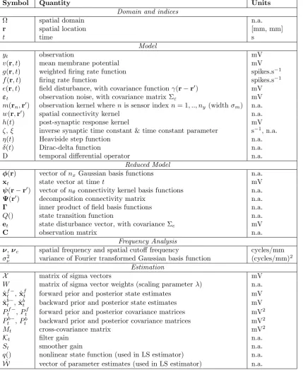
The combination of modeling techniques in this paper leads to a large amount of notation, so a reference

of the symbols used is provided in Table 1. The model relates the average number of action potentialsg(r, t)

Symbol Quantity Units

Domain and indices

Ω spatial domain n.a.

r spatial location [mm, mm]

t time s

Model

yt observation mV

v(r, t) mean membrane potential mV

g(r, t) weighted firing rate function spikes.s−1

f(r, t) firing rate function spikes.s−1

e(r, t) field disturbance, with covariance functionγ(r−r′

) mV

εt observation noise, with covariance matrix Σε mV

m(rn,r′) observation kernel wherenis sensor index n= 1, .., ny (widthσm) n.a. w(r,r′

) spatial connectivity kernel n.a.

h(t) post-synaptic response kernel mV

ζ, ξ inverse synaptic time constant & time constant parameter s−₁

, n.a.

η(t) Heaviside step function n.a.

δ(t) Dirac-delta function n.a.

D temporal differential operator n.a.

Reduced Model

φ(r) vector ofnxGaussian basis functions n.a.

x_t state vector at timet mV

ψ(r−r′

) vector ofnθconnectivity kernel basis functions n.a.

Ψ(r′

) decomposition connectivity matrix n.a.

Γ inner product of field basis functions n.a.

Q() state transition function n.a.

et state disturbance vector, with covariance Σe mV

C observation matrix n.a.

Frequency Analysis

ν, νc spatial frequency and spatial cutoff frequency cycles/mm σ2

ν variance of Fourier transformed Gaussian basis function (cycles/mm)2 Estimation

X matrix of sigma vectors mV

W matrix of sigma vector weights (scaling parameterλ) n.a. ˆ

xf_t−, ˆxf_t forward prior and posterior state estimates mV ˆ

xb_t−, ˆxb

t backward prior and posterior state estimates mV

Ptf−, Ptf forward prior and posterior covariance matrices mV2 Pb−

t ,Ptb backward prior and posterior covariance matrices mV2

Mt cross-covariance matrix mV2

Kt filter gain n.a.

St smoother gain n.a.

q() nonlinear state function (used in LS estimator) n.a. ˆ

W vector of parameter estimates (used in LS estimator) n.a.

Table 1: Notation.The first column of the table gives the symbols for all the notation used in the paper. The second column

arriving at time t and position r to the local post-synaptic membrane voltage v(r, t). The post-synaptic

potentials generated at a neuronal population at location r by action potentials arriving from all other

connected populations is described by

v(r, t) =

Z t

−∞

h(t−t′)g(r, t′)dt′. (1)

The post-synaptic response kernelh(t) is described by

h(t) =η(t) exp (−ζt), (2)

whereζ=τ−1_{,τis the synaptic time constant andη(t) is the Heaviside step function. Non-local interactions}

between cortical populations at positionsrandr′

are described by

g(r, t) =

Z

Ω

w(r,r′)f(v(r′, t))dr′, (3)

where f(·) is the firing rate function, w(·) is the spatial connectivity kernel and Ω is the spatial domain

representing a cortical sheet or surface. The connectivity kernel is typically a “Mexican hat” or “wizard

hat” function, which describes local excitation and surround inhibition. An example of the Mexican hat

connectivity kernel, that is a weighted sum of Gaussians, used in this paper is shown in Fig. 1. To

demon-−10 0 10

Space

−50 0 50 100

C

o

n

n

e

ct

io

n

S

tr

e

n

g

th

Figure 1: Mexican-hat connectivity kernel. The kernel is a composite of three Gaussian basis functions (dashed lines),

representing short-range excitation, mid-range inhibition and long-range excitation. The kernel is rotationally symmetric (isotropic) about zero, hence a cross-section captures the important aspect of the connectivity kernel’s shape. The kernel decays asymptotically to zero.

strate flexibility in the estimation algorithm and to model larger cortical regions, a third component of the

kernel is introduced describing weak longer-range excitation. The exact shape of this kernel is assumed to

vary across subjects, and hence needs to be inferred from subject-specific data.

sigmoidal activation function

f(v(r′, t)) = 1

1 + exp (ς(v0−v(r′, t)))

. (4)

The parameter v0 describes the firing threshold of the neural populations and ς governs the slope of the

sigmoid. By substituting equation 3 into equation 1 we get the spatiotemporal model

v(r, t) =

Z t

−∞

h(t−t′

)

Z

Ω

w(r,r′)f(v(r′, t′

))dr′dt′

. (5)

To obtain the standard integro-differential equation form of the model, we use the fact that the synaptic

response kernel is a Green’s function of a linear differential equation defined by the differential operator

D =d/dt+ζ. A Green’s function satisfies

Dh(t) =δ(t), (6)

whereδ(t) is the Dirac-delta function. Applying the differential operator D to equation 1 gives

Dv(r, t) = D (h∗g) (r, t) (7)

= (Dh∗g) (r, t) (8)

= (δ(t)∗g) (r, t) (9)

=g(r, t) (10)

where∗denotes the convolution operator. This gives the standard form of the model

dv(r, t)

dt +ζv(r, t) = Z

Ω

w(r,r′)f(v(r′, t))dr′. (11)

To arrive at the integro-difference equation (IDE) form of the model, we discretize time using a first-order

Euler method (see Appendix A for derivation) giving

vt+Ts(r) =ξvt(r) +Ts Z

Ω

w(r,r′)f(vt(r

′

))dr′+et(r), (12)

whereTsis the time step,ξ= 1−Tsζandet(r) is ani.i.d.disturbance such thatet(r)∼ GP(0, γ(r−r

′

)). Here

GP(0, γ(r−r′

)) denotes a zero mean Gaussian process with spatial covariance functionγ(r−r′

) (Rasmussen

and Williams (2005)). The disturbance is added to account for model uncertainty and unmodeled inputs.

To simplify the notation, the index of the future time sample,t+Ts, shall be referred to ast+ 1 throughout

the rest of the paper.

using the observation function that incorporates sensors with a spatial extent by

yt(rn) =

Z

Ω

m(r_n−r′)vt(r

′

)dr′+εt(rn), (13)

where m(rn−r′) is the observation kernel, rn defines the location of the electrodes in the field, n =

0, ..., ny−1 indexes the sensors and εt(rn) ∼ N(0,Σε) denotes a multivariate normal distribution with

mean zero and the covariance matrix Σε =σ2εI, where Iis the identity matrix. Since we are considering

intracranial measurements recorded directly from the surface of the cortex or within the brain, the lead field

is not modeled by the observation equation.

When considering the measurement of a point source in a conductive homogeneous field measured by a

point sensor, the observation kernel will theoretically follow a Laplacian like shape, with an exponential decay

in the amplitude of a measurement with an increasing distance between the source and sensor (Jackson,

1999). However, when considering a source or sensor with a spatial extent, the peak of the observation kernel

becomes smoothed and is more similar to a Gaussian shape (Jackson, 1999). An experiment supporting this

was performed and the results are shown in Appendix B. Therefore, in this study the observation kernel,

m(r−r′), that governs the sensor pick-up geometry is defined by the Gaussian

m(r−r′) = exp

−(r−r ′

)⊤

(r−r′

) σ2

m

, (14)

whereσmsets the kernel width. The superscript⊤denotes the transpose operator.

2.3. Derivation of Finite Dimensional State-Space Model

In order to implement standard estimation techniques, we use a decomposition of the field using a

set of Gaussian basis functions. Decomposition allows a continuous field to be represented by a

finite-dimensional state vector. This facilitates application of standard nonlinear state estimation methods such

as the unscented Kalman filter. The field decomposition is described by

vt(r)≈φ

⊤

(r)xt, (15)

wherextis the state vector that scales the field basis functionsφ(r). The field basis functions are described

by

φ(r−r′) = exp −(r−r ′

)⊤

(r−r′

) σ2

φ

!

, (16)

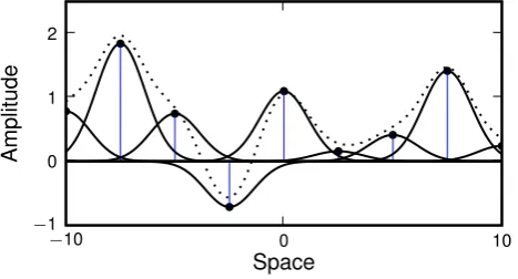
where σφ is the basis function width parameter. An example of a one-dimensional field decomposition is

given in Fig. 2. The width and positioning of the basis functions can be determined by spectral analysis

−10 0 10

Space

−1 0 1 2

A

m

p

lit

u

d

e

Figure 2: Example of a one-dimensional field decomposition. A continuous, one-dimensional field decomposed by a

finite number of basis functions scaled by the state vector. The dashed line depicts the field, the black solid lines show the Gaussian basis functions and the vertical lines show the position and amplitude of the states.

The connectivity kernel can also be decomposed as

w(r,r′) =ψ⊤(r,r′)θ, (17)

whereψ(r,r′

) is a vector of Gaussian basis functions andθ is a vector of scaling parameters. A graphical

demonstration of the connectivity kernel decomposition and the net shape is provided in Fig. 1. By exploiting

the isotropy of the connectivity basis functions, they can be written asψ(r−r′). We will assume that we

know the parametric form of the connectivity basis functions, where the scaling parametersθ are unknown.

Note, that although most examples presented in this paper use the Mexican hat connectivity kernel, the

framework is also valid for other connectivity kernels, provided they are homogeneous and that they can be

approximated by a set of isotropic basis functions parametrized by a coefficient vectorθ. The mathematical

formulation does not restrict the shape of the kernel, where anisotropic arbitrary shapes can be represented.

Furthermore, the kernel basis functions need not be a Gaussian shape, but can be, for example, Laplacian

to describe the “wizard hat” connectivity or B-spline functions to describe a kernel with a compact support.

Each connectivity basis function of the Mexican hat can, individually, be considered a layer in the

Wilson and Cowan model. Rearranging the order of the spatial convolution in equation 12 and substituting

in equations 15 and 17 to the right hand side we get the approximation of the dynamic field

vt+1(r)≈Ts

Z

Ω

f(φ⊤(r′)xt)ψ⊤(r−r′)dr′θ

Next we cross-multiply equation 18 byφ(r) and integrate over the spatial domain, Ω, to get

Z

Ω

φ(r)vt+1(r)dr

≈Ts

Z

Ω

φ(r)

Z

Ω

ψ⊤(r−r′)f(φ⊤(r′)xt)dr′drθ

+ξ Z

Ω

φ(r)φ⊤(r)drx_t+

Z

Ω

φ(r)et(r)dr. (19)

The solution of this equation for xt is equivalent to finding a Galerkin projection, where the field basis

functions would be considered the projection functions and the states would be the amplitude coefficients.

See Appendix C for more information. In the next step of forming the state-space model we substitute the

field decomposition into the left hand side of equation 19 giving

Z

Ω

φ(r)φ⊤(r)xt+1dr

=Ts

Z

Ω

φ(r)

Z

Ω

ψ⊤(r−r′)f(φ⊤(r′)xt)dr′drθ

+ξ Z

Ω

φ(r)φ⊤(r)drxt+

Z

Ω

φ(r)et(r)dr. (20)

Now defining the matrix

Γ, Z

Ω

φ(r)φ⊤(r)dr, (21)

and substituting it into equation 20 and cross-multiplying byΓ−1 gives

xt+1=TsΓ

−1Z

Ω

φ(r)

Z

Ω

ψ⊤(r−r′)f(φ⊤(r′)xt)dr′drθ

+ξxt+Γ

−₁Z

Ω

φ(r)et(r)dr. (22)

The analytic derivation of the inner product ofn-dimensional Gaussians, which was used for calculatingΓ,

is provided in Appendix D. Alternative field basis functions may be used to form the decomposition; if

the basis is orthonormal, such as a Fourier basis, then Γ is simply the identity matrix. Equation 22 can be

simplified by exploiting the isotropy of the connectivity kernel basis functions where

ψi(r−r

′

) =ψi(2ci+r

′

−r) (23)

and c_i is the center of the ith _{basis function of the kernel decomposition. To make the simplification we}

define

[Ψ(r′)]:i,TsΓ

−1Z

Ω

where [Ψ(r′

)]_:i denotes theith_{column ofΨ(r}′

) which is anx×nθmatrix, wherenxis the number of basis

functions (states) and nθ is the number of connectivity kernel basis functions. This matrix is pre-defined

analytically (see Appendix E for analytic convolution of two Gaussians), since it is constant with respect

to the states and the unknown parameters. SubstitutingΨ(r′

) into equation 22 gives

xt+1= Z

Ω

Ψ(r′)f(φ⊤(r′)xt)dr′θ

+ξxt+Γ

−1Z

Ω

φ(r)et(r)dr. (25)

This substitution swaps the convolution in equation 18, which is computationally demanding, with the

convolution in equation 24, which is pre-defined analytically. This is of great importance as it lowers the

computational demands of the estimation algorithm and provides a dramatic increase in estimation speed.

Now we define the state disturbance as

e_t,Γ−1 Z

Ω

φ(r)et(r)dr, (26)

which is a zero mean normally distributed white noise process with covariance (see Appendix F for the

derivation)

Σe=Γ

−1Z

Ω Z

Ω

φ(r)γ(r−r′)φ(r′)⊤ dr′drΓ−⊤. (27)

The observation equation of the reduced model is found by substituting equation 15 into equation 13 giving

y_t=

Z

Ω

m(r_n−r′)φ⊤(r′)x_tdr′+εt. (28)

Note, the sensor indexrn has been omitted to delineate the reduced model observation equation from the

full model. The observation equation is linear and can be written in the more compact form

yt=Cxt+εt, (29)

where each element of the observation matrix is

C_{ij ,} Z

Ω

m(r_i−r′)φ_j(r′)dr′. (30)

Now we have the final form of the state-space model where

xt+1=Q(xt) +et (31)

and

Q(xt) =

Z

Ω

Ψ(r′)f(φ⊤(r′)xt)dr′θ+ξxt. (33)

2.4. Spectral Analysis

Spectral analysis has been used to identify both the number of sensors and the number of basis functions

required to reconstruct the neural field from sampled observations (Sanner and Slotine, 1992; Scerri et al.,

2009). Based on a two-dimensional extension of Shannon’s sampling theorem (Peterson and Middleton,

1962), the spatial bandwidth of the observed field can be used to provide a lower bound on both the number

of sensors and the number of basis functions required to capture the dominant spatial spectral characteristics

of the neural field.

Let the spectral representation of the post-synaptic membrane voltage field at time t be denoted by

Vt(ν), where ν is the spatial frequency. According to Shannon’s sampling theorem, the field must be

spatially band-limited for an accurate reconstruction using spatially discrete observations. However, an

approximate reconstruction can be obtained if the field is approximately band-limited with

Vt(ν)≈0 ∀ν>νc, (34)

where νc is a cutoff frequency (typically taken as the -3 dB point). Given such a band-limited field, the

distance between adjacent sensors, ∆y, must satisfy

∆y ≤ 1 2ρyνc

, (35)

where ρy ∈ R≥ 1 is an oversampling parameter. A derivation of the sampling theorem that is based on

Sanner and Slotine (1992) and Scerri et al. (2009) is provided in Appendix G. The condition in equation 35

must be satisfied to avoid spatial spectral aliasing effects when reconstructing the hidden dynamic field,

vt(r), using the sampled observations, yt.

In practice, it is difficult to estimate the bandwidth of the cortex using traditional electrophysiological

measurements, possibly preventing placement of sensors in accordance to equation 35. However, we envisage

it may be possible to estimate the spatial bandwidth using other modalities with higher spatial resolution

such as fMRI, NIRS or other optical imaging techniques (Issa et al. (2000)). The expected bandwidth of

the human neocortex is approximately 0.1-0.4 cycles/mm (Freeman et al., 2000).

Spectral aliasing can be avoided by a proper choice of the spatial sampling distance given the sensors’

spectral characteristics. The spatial extent of the sensors results in a spectral low-pass action, thus providing

spatial anti-aliasing filtering. Such sensors limit the spatial bandwidth of the observation to a value denoted

byνcy. Aliasing can then be avoided by positioning the sensors according to equation 35, replacingνc with

Although such sensors avoid errors due to aliasing, they attenuate the high spatial frequency variations

in the observations. Therefore, any procedure applied to estimate the original field or the underlying

connectivity structure from these band-limited observations has the potential to underestimate the high

spatial frequency components of both the field and the connectivity kernel. This motivates the use of

sensors with wider bandwidths (narrower in space). This choice would require more sensors in order to

satisfy Shannon’s sampling theorem for a given spatial region. Therefore, a compromise should be found

between the bandwidth of the sensor response, the accuracy of the estimation results, the number of sensors

and the computational demands of the estimation procedure when designing experiments.

Similar considerations need to be made regarding the representation of the dynamic field, vt(r), using

the basis function decomposition. Again, applying Shannon’s sampling theorem, the maximum distance

between basis functions to accurately reconstruct the neural field must satisfy

∆φ≤ 1

2ρφνcy

(36)

whereρφ∈R≥1 is an oversampling parameter to determine the basis function separation.

The field basis function widths can also be inferred using spectral considerations (Sanner and Slotine,

1992; Scerri et al., 2009). To demonstrate this, we begin with a two-dimensional Gaussian basis function

located at the origin, defined as

φ(r) = exp − 1 σ2

φ

r⊤r !

. (37)

The corresponding Fourier transform is

Φ(ν) =

₁

πσ2

ν

exp

− 1

σ2

ν

ν⊤ν

, (38)

where

σν2= 1 π2_σ2

φ

. (39)

To obtain a 3 dB attenuation atνcy, the basis function width,σ2φ, should be chosen such that

σ2_φ= 1 π2_σ2

νcy

, (40)

where

σ2_νcy = 2ν

⊤

cyνcy

ln 2 . (41)

This ensures that the basis functions can represent the neural field with frequency content up to νcy.

Derivations for equations 38 and 41 are given in Appendix H.

approx-imated field by reducing the spatial bandwidth. This allows for an approximate representation by a lower

order model (fewer basis functions), thus reducing the computational demands of the estimation process.

The spatial cutoff frequency of this smoothed field becomes a design choice. To calculate the cutoff frequency

imposed by the basis function width, we rearrange equations 40 and 41 giving

νcφ= 1 πσφ

r

ln 2

2 . (42)

Note that for a spatially homogeneous and isotropic field, the basis functions can be placed on a regular

grid. Thus, the knowledge of the distance between basis functions can be used to determine the total number

of basis functions required to represent a known spatial region.

2.5. State and Parameter Estimation

In this section, we describe the procedure for estimating the states,xt, the connectivity kernel parameters,

θ, and the synaptic dynamics,ξ. The framework assumes that the parameters of the model (and brain) are

stationary over the estimation period. This is a reasonable assumption when applying the framework to an

evoked-potential experiment over a short time period in a controlled environment.

The estimation process is a two part iterative algorithm, consisting of a state estimation step followed

by a parameter estimation step. Once initialized, at each iteration the sequence of estimated state vectors

is used to update the parameter set. The resulting parameters are then used when estimating the new

state vector sequence for the next iteration. The procedure stops when the parameter estimates converge.

The algorithm is initialized using a bounded random state vector sequence, guaranteeing that the initial

estimated parameter set forms a stable kernel.

The additive form of the unscented Rauch-Tung-Striebel smoother (URTSS) (Sarkka, 2010) was used

for the state estimation. The URTSS incorporates an unscented Kalman filter (UKF) (Julier and Uhlmann,

1997; van der Merwe, 2003) in a forward step to estimate posterior states, ˆxf_t, followed by a backward step

to compute the smoothed state estimates, ˆxb_t. The first and second order moments of the predicted state

are captured by propagating the so-called sigma points through the state equation. The sigma points,Xi,

are calculated using the unscented transform as follows:

X0=x¯ (43)

Xi =x¯+

p

(nx+λ)Px

i, i= 1, . . . , nx (44)

Xi =x¯−

p

(nx+λ)Px

i−_n x

, i=nx+ 1, . . . ,2nx (45)

where ¯x represents either ˆxf_t or ˆxb_t, Px is the corresponding covariance matrix for filtering or smoothing,

_p

(nx+λ)Px

i is the i

th _{column of the scaled matrix square root ofPx, andn}

state space. The total number of sigma points is 2nx+ 1. The scaling parameter,λ, is defined as

λ=α2(nx+κ)−nx, (46)

The positive constantα, that determines the spread of the sigma points around ¯x, was set to 10−3_{. It is}

typically set arbitrary small to minimise higher-order effects (Haykin, 2001). The other scaling parameter,

κ, was set to 3−nxin accordance to Julier et al. (2002).

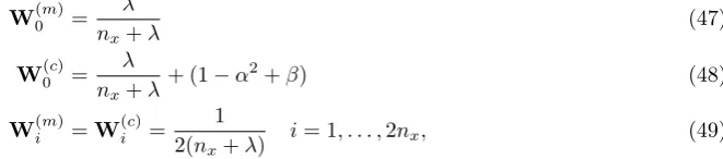
The sigma vectors are propagated through the system equations and weighted to form the predicted

mean and covariance. The weights are calculated by

W(₀m)= λ nx+λ

(47)

W(₀c)= λ nx+λ

+ (1−α2+β) (48)

W(_im)=W_i(c)= 1 2(nx+λ)

i= 1, . . . ,2nx, (49)

where the superscripts m and c denote mean and covariance and β incorporates prior knowledge of the

distribution of the states, x(for a Gaussian disturbance, β should be set to 2 (Haykin, 2001)). Since the

observation equation is linear (equation 29), the standard Kalman Filter update equations are used to correct

the predicted states. The state estimates from forward filtering are used to form a new set of sigma points

for the smoother, as described above. The cross-covariance matrix of the states, M, is also required for

computing the smoother gain, as described in the summary of the steps in the URTSS algorithm given in

Table 2.

Although the system is nonlinear, the parameters of the system are linear with respect to the state.

This is exploited by our procedure where the parameter estimation uses a least squares (LS) method that

minimizes the sum of the squared errors (of a predicted state update) with each new estimate of the state

vector sequence. To create the least squares parameter estimator, we first define thenx×nθmatrix

q(xt) =

Z

Ω Ψ(r′

)f(φ⊤(r′

)xt) dr′

. (50)

Now given a state estimate sequence from the initialization or an iteration of the URTSS, we can write

ˆ

xb₁=q(ˆxb₀)θ+ξxˆb₀+e0

ˆ

xb₂=q(ˆxb₁)θ+ξxˆb₁+e1

.. .

ˆ

1. Forward initialization

ˆ

x0,P0

2. Forward iteration: for t ∈ {0,· · · , T}, calculate the sigma points X_i,tf using equations 43-46 and propagate through equation 33

X_i,tf−₊₁=Q(X_i,tf) i= 0, . . . ,2nx

Calculate the predicted state and the predicted covariance matrix

ˆ

xf_t+1− =P2nx

i=0W (m)

i X

f−

i,t+1

Pf_t+1− =P2nx

i=0W (c)

i (X f−

i,t+1−xˆ

f−

t+1)(X

f−

i,t+1−ˆx

f−

t+1) ⊤

+Σe

Compute the filter gain, the filtered state and the filtered covariance matrix using the standard Kalman filter update equations

Kt+1=Pf −

t+1C ⊤

(CPf_t+1−C⊤

+Σε)−₁

ˆ

xf_t+1= ˆxf_t+1− +Kt+1(yt+1−Cˆxf −

t+1)

Pf_t+1= (I− Kt+1C)Pf −

t+1

3. Backward initialization

Pb T =P

f

T, xˆbT = ˆx f T

4. Backward iteration: fort∈ {T−1,· · · ,0}calculate the sigma pointsXb

i,tand propagate them through equation 33

Xb−

i,t+1=Q(Xi,tb ) i= 0, . . . ,2nx Calculate the predicted state and the predicted covariance matrix

ˆ

xb_t+1− =P2nx

i=0W (m)

i X

b−

i,t+1

Pb_t+1− =P2nx

i=0W (c)

i (Xb

−

i,t+1−xˆb −

t+1)(Xb −

i,t+1−ˆxb −

t+1) ⊤

+Σe

M_t+1=P2_i=0nxW_i(c)(Xi,tb −xˆ f t)(Xb

−

i,t+1−xˆb −

t+1) ⊤

Compute the smoother gain, the smoothed state and the smoothed covariance matrix

S_t=M_t+1Pb −

t+1 −1

ˆ

xb t = ˆx

f

t +Stxˆbt+1−xˆb −

t+1

Pb t=P

f t +St

Pb

t+1−Pb −

t+1

S⊤

t

Table 2:Algorithm for the Unscented RTS Smoother. This table shows the steps in the unscented Rauch-Tung-Striebel

smoother algorithm. The steps are iterated 10 times for our state estimation procedure. The least squares algorithm is run after each iteration to update the parameter estimates.

This can be written in the compact form

where Z=         ˆ

xb1

ˆ

xb2

.. .

ˆ

xbT        

, X=

       

q(ˆxb0) ˆx

b

0

q(ˆxb1) ˆx

b

1

..

. ...

q(ˆxb T₋1) xˆ

b T₋1

        and W=   θ ξ 

, e=         e0 e1 .. .

eT₋1

        .

Following this, the LS parameter estimates (Ljung, 1999), ˆW, are

ˆ

W= (X⊤X)−1X⊤Z. (52)

3. Results

We now provide demonstrations of the estimation procedure using the new methods that are described

above. Data was generated using the neural field model, described in Section 2.2, to demonstrate the state

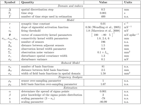
and parameter estimation framework. All parameters for the model are given in Table 3, unless otherwise

explicitly stated for particular experiments. Note that the parameters for the spatial and temporal aspects of

the model can be considered arbitrary when demonstrating the estimation methodology. This is because the

temporal aspects scale with the sampling rate and the length of the times series, and the spatial aspects scale

with the size of the neural field and the spatial step size used for numerical simulation. When generating

the simulated data, we assumed free boundary conditions for the neural field. An example of the simulated

field at a single point in time can be seen in Fig. 3(A). Fig. 3(B) shows an example of data from the modeled

sensors and Fig. 3(C) shows the power spectral density (PSD) of the simulated time-series.

The sensors were spaced on a 14×14 square grid and the sensor width was set to σ2

m = 0.81. This

provides a width of 1.5 mm at half the maximum amplitude of the observation kernel. The distance between

sensors was set to ∆y = 1.5 mm. This arrangement modeled the recording as having some cross talk (from

volume conduction), which is typical for neurophysiological recordings.

3.1. Spatial Frequency Analysis

The spectral analysis was used to confirm that the spacing and width of the sensors was adequate to

capture the significant dynamics of the field. Fig. 4(A) shows the spatial frequency of the neural field and

Fig. 4(B) shows the spatial frequency of the reconstructed neural field from the basis function decomposition.

Symbol Quantity Value Units

Domain and indices

∆ spatial discretisation step 0.5 mm

Ts time step 0.001 s

T number of time steps used in estimation 400 n.a.

Model

τ synaptic time constant 0.01 s−1

ς slope of sigmoidal activation function 0.56 (Wendling et al., 2005) mV−1

v0 firing threshold 1.8 (Marreiros et al., 2008) mV

θ vector of connectivity kernel parameters

100 −80 5 ⊤

mV.spike−₁

σψ1, σψ2, σψ3 connectivity kernel width parameters 1.8, 2.4, 6 mm

ny number of sensors 196 n.a.

∆y distance between adjacent sensors 1.5 mm

σm observation kernel width parameter 0.9 mm

Σε observation noise variance 0.1×Iny mm

2

σγ disturbance spatial covariance width 1.3 mm

σd disturbance variance 0.1 mV

Reduced Model

nx number of basis functions 81 n.a.

∆φ distance between field basis functions 2.5 mm

σφ width of field basis functions in spatial domain 1.58 mm2 Frequency Analysis

ρy sensor over-sampling parameter 1 n.a.

ρφ field basis function over-sampling parameter 1.67 n.a.

Estimation

α determines the spread of sigma points 0.001 n.a.

β prior knowledge of the sigma points distribution 2 n.a.

κ scaling parameter (3−nx) -78 n.a.

λ scaling parameter -80.99 n.a.

Table 3: Parameters. Parameters for the neural field model, the reduced model, the frequency analysis and the estimation

0 10 Space -10 0 10 S p a ce −1.8 0.0 2.4 50ms 8 m v C h a n n e ls

B

A

C

100 ₁₀1 ₁₀2

Frequency (Hz) 15 20 25 30 35 40 45 P o w e r (d B )

Figure 3: Example of the spatiotemporal properties of the model and synthetically generated data. (A)The

neural field at a single time instant. (B) Data generated by the full neural field model at the first 5 sensors. (C) Mean power

spectral density of the data generated by the observations.

2 0 2 S p a ti a l F re q . Spatial Freq.

A

2 0 2 S p a ti a l F re q . Spatial Freq.

B

Figure 4:Spatial frequency analysis: the neural field. (A) The average (over time) power in dB of the spatial frequency

of the neural field. (B) The average (over time) power in dB of the spatial frequency of the reconstructed neural field from the

a maximum sensor separation of 2.08 mm. This confirms that the separation of ∆y= 1.5 mm was sufficient

to mitigate problems associated with spatial aliasing of the dominant dynamics.

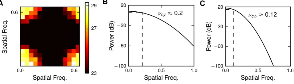
The spatial frequency of the observed field is shown in Fig. 5(A). The cutoff frequency isνcy ≈0.2

cy-0.0 0.5 1.0

Spatial Freq. −100 −60 −20 20 P o w e r (d B )

νcφ≈0.12

C

0.0 0.5 1.0

Spatial Freq.

−100 −60 −20 20

νcy ≈0.2

P o w e r (d B )

B

A

Figure 5: Spatial frequency analysis: observations and basis functions. The dashed line shows the cutoff frequency

(−3 dB point). (A) The average (over time) power in dB of the spatial frequency of the observations. (B) The spatial

frequency response of a one-dimensional model sensor. The symmetry of the sensors and field basis functions allow for the

one-dimensional representation of the spectral characteristics. (C) The spatial frequency response of a one-dimensional neural

field basis function, illustrating a narrower band width than the sensors.

cles/mm (−3 dB point). The observation cutoff frequency is lower than the field cutoff due to the low-pass

filtering effect of the sensors. The spatial frequency response of the sensors can be seen in Fig. 5(B).

As described in Section 2.4, the basis function configuration can be systematically chosen to account

for the full spatial bandwidth from the observations, or alternatively, the configuration can be chosen to

represent the neural field up to a specified bandwidth to limit the computational complexity of the estimation

procedure. In the examples provided in this paper, the later option was chosen, where the neural field cutoff

frequency was further reduced toνcφ= 0.12 cycles/mm. The band-limiting effect on the field reconstruction

can be seen by comparing Fig. 4(A) to Fig. 4(B). This effect is due to the spatial frequency response of the

basis functions, which is shown in Fig. 5(C). Due to the slow roll-off in the frequency response of Gaussian

basis functions an oversampling parameter of ρφ = 1.67 was chosen. Given the spectral response of the

basis functions, the over-sampling parameter, and the spatial domain an equally spaced grid of 9×9 basis

functions was used to decompose the field, which resulted in 81 states.

3.2. State and Parameter Estimates

Several experiments were performed to demonstrate the performance of the state and parameter

estima-tion algorithm. The first experiment evaluated the estimaestima-tion performance using a Monte Carlo approach

for a single set of parameters. In this experiment we demonstrate convergence of the algorithm, show the

The second experiment evaluated the performance with a selection of different connectivity kernel

parame-ters. In addition, results are shown where the support of the connectivity kernels differs between actual data

and the estimator. The third experiment shows how the estimation accuracy depends on the parameters of

the sigmoidal nonlinearity. The final experiment shows the effect of the width of the observation kernel on

the estimation performance.

3.2.1. Experiment I: Monte Carlo Simulation with Fixed Parameters

A Monte Carlo approach was employed where 150 realizations of the data were generated, such that

distributions of the parameters estimates could be formed. Each realization consisted of 500 ms of data

(sampled at 1 kHz) and the estimation was applied to the final 400 ms, allowing the model’s initial transients

to die out. The initial state and parameters were unknown to the estimator. Ten iterations of the estimation

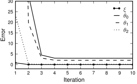
algorithm were used to ensure that the parameter estimates converged. Fig. 6 shows the rate of convergence,

confirming that the algorithm converged to steady parameter values, with the changes in the parameter errors

(between consecutive iterations) falling to less than 10−₄

after 6 iterations.

1 2 3 4 5 6 7 8 9 10

Iteration

0 5 10 15 20 25 30

E

rr

o

r

ξ θ0 θ1 θ2

Figure 6: Convergence of parameters. The mean of the absolute error between true and estimated parameters averaged

over 150 realizations. All parameters converge after 6 iterations, where the mean difference between errors in consecutive

iterations falls below 10−4

.

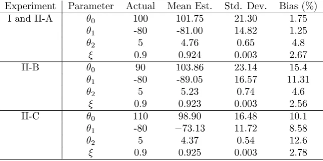
Histograms of the parameter estimates obtained over the 150 realizations are shown in Fig. 7. In each

of the subplots of the figure the true parameter value is shown by the solid line and the mean parameter

estimate is shown by the dashed line. The actual parameter values, the mean parameter estimates, standard

deviations, and biases for this parameter combination are given as the first entry in Table 4, where other

entries in the table show results from Experiment II. The biases show the percentage differences between the

actual values and the mean parameter estimates. For this parameter combination the mean estimates are in

good agreement (within 1 standard deviation) with the actual values of the connectivity kernel parameters.

However, the time constant parameter,ξ, is outside the estimated distribution (with bias of 2.67%), with

40 100 160

ˆ

θ0 0

20 40

A

B

C

D

−130 −90 −50

ˆ

θ1 0

20 40

3.0 5.0 6.5

ˆ

θ2 0

20 40

0.85 0.90 0.95

ˆ

ξ 0

35 70

Figure 7: Histograms of the parameter estimates over 150 realizations. In each of the subplots the solid lines show

the actual parameter values and the dotted lines show the means of the estimated parameters. (A) The histogram of the

central excitatory connectivity kernel basis function parameter estimates,θ0. (B) The histogram of the surround inhibition

connectivity kernel basis function parameter estimates, θ1. (C) The histogram of the longer range excitatory connectivity

kernel basis function parameter estimates,θ2. (D) The histogram of theξestimates whereξ= 1−ζTsandζis the reciprocal

of the synaptic time constant.

Experiment Parameter Actual Mean Est. Std. Dev. Bias (%)

I and II-A θ0 100 101.75 21.30 1.75

θ1 -80 -81.00 14.82 1.25

θ2 5 4.76 0.65 4.8

ξ 0.9 0.924 0.003 2.67

II-B θ0 90 103.86 23.14 15.4

θ1 -80 -89.05 16.57 11.31

θ2 5 5.23 0.74 4.6

ξ 0.9 0.923 0.003 2.56

II-C θ0 110 98.90 16.48 10.1

θ1 -80 −73.13 11.72 8.58

θ2 5 4.37 0.54 12.6

ξ 0.9 0.925 0.003 2.78

components in the smoother estimated field with respect to the actual field. These results indicate that

choosing to limit the frequency content of the reconstructed neural field has only minor effects on the

accuracy of the estimated kernel while allowing for significant gains in the computational demand.

The accuracy of the state estimates was evaluated by comparing the field reconstruction to the true

field using the mean (over iterations) of the root mean square error (MRMSE) over space. The MRMSE

of the field estimates over time for 150 realizations is shown in Fig. 8 with the 95 % confidence interval.

At each time point, the error is consistently around 0.5 mV, which is approximately 10.73 % of the field

0.1 0.2 0.3 0.4 0.5

Time (sec)

0.49 0.50 0.51 0.52

M

R

M

S

E

Figure 8: Error in the field reconstruction. The mean (over iterations) of average (over space) RMSE of the estimated

field over 150 realizations (solid line) and the 95 % confidence interval (grey region).

voltage range ([-2.20, 2.46] mV). The error in the reconstructed field is again mostly due to the loss of high

spatial frequency information from the basis function decomposition as illustrated in Fig. 9. The figure

0 10

−10 0 10

S

p

a

ce

Space

A

−1.5 0.0 2.0

0 10

−10 0 10

S

p

a

ce

Space

B

−1.5 0.0 2.0

0 10

−10 0 10

S

p

a

ce

Space

C

−1.5 0.0 2.0

Figure 9: Examples of the actual and estimated neural fields and the error. (A) The actual field at a single time

instant from the neural field model that was used to generate the data. (B) The reconstructed field of the reduced model,

showing the effect of the basis function decomposition on the frequency content of the estimated field. (C) The error between

the true and reconstructed fields.

shows a snapshot at a single time instant of the true neural field, the estimated field, and the corresponding

the estimated field contains the basic structure of the true field, shown in Fig. 9(A), but is missing the

higher-frequency detail, which can be see in the error shown in Fig. 9(C).

3.2.2. Experiment II: Results for Different Connectivity Kernel Parameters

To study the robustness of the estimation algorithm, the performance was evaluated for various

connec-tivity kernel parameters. The reconstructed connecconnec-tivity kernels from the estimated parameters are shown

in Fig. 10. For Fig. 10(A-C) Mexican hat connectivity kernels were used. For each subset of parameters,

−20 0 40

θ0=100 θ1=-80 θ2=5

A

θ0=90 θ1=-80 θ2=5

B

θ0=110 θ1=-80 θ2=5

C

−10 0 10

Space 0 60 C o n n e ct io n S tr e n g th

θ0=15 θ1=0 θ2=0

D

−10 0 10

Space

θ0=30 θ1=0 θ2=0

E

−10 0 10

Space

θ0=50 θ1=0 θ2=0

F

Figure 10: Cross-section of connectivity kernel estimates. In each of the subplots the actual kernels are shown by the

solid lines, the mean kernel estimates (over 50 realizations) are shown by the dotted lines and the 95 % confidence intervals are shown by the shaded grey regions.

the mean of the reconstructed kernel over 50 realizations is shown as a dotted line and the 95 % confidence

interval is indicated by the grey shaded region. In each case, the actual kernel was within the 95 % confidence

interval of the kernel estimate. The statistics for the kernel parameter estimates for each of the parameter

sets are shown in Table 4.

For each of the Mexican hat connectivities, the support of the kernel was assumed to be known. However,

in Fig. 10(D-F) the kernel support in the estimator differed from the actual data. In these cases the data sets

were generated using a single positive (excitatory) Gaussian kernel, as seen by the solid line in each of the

subplots of the figure. The estimation algorithm was constructed allowing for the Mexican hat connectivity

of the previous examples. Each plot shows that the actual kernel lies within the confidence intervals of the

Table 5 shows the statistics of the parameter estimates. Although the net reconstructed kernel estimates

Experiment Parameter Actual Mean Est. Std. Dev. Bias (%)

II-D θ0 15 35.68 16.72 137.87

θ1 0 −18.16 11.77

-θ2 0 0.81 0.53

-ξ 0.9 0.923 0.002 2.56

II-E θ0 30 40.43 11.47 34.77

θ1 0 −12.01 7.8

-θ2 0 0.35 0.36

-ξ 0.9 0.924 0.003 2.67

II-F θ0 50 61.46 11.51 22.92

θ1 0 −15.03 7.56

-θ2 0 0.27 0.29

-ξ 0.9 0.924 0.003 2.67

Table 5: Results from varying the Gaussian connectivity kernel parameter

are in good accordance with the actual kernels, the individual kernel basis function weights are not in

agreement with the actual parameters. This result demonstrates that the interpretation of the results

should be based on the net shape of the estimated connectivity kernel and not on the estimated parameter

values individually. These results indicate that the solution to the system may not be unique in non-ideal,

practical situations. Nevertheless, the net shape of the connectivity kernel can be determined reasonably

accurately.

3.2.3. Experiment III: Results for Varying the Parameters of the Sigmoidal Activation Function

Fig. 11 demonstrates the effect of the sigmoid parameters on the estimation accuracy. The RMSE of the

reconstructed connectivity kernel was calculated for various parameters of the sigmoid by varying the slope,

ς, and the threshold,v0. The other model parameters remained fixed and were set according to the Table 3.

From Fig. 11 it can be seen that the estimation accuracy depends on the parameters of the sigmoid

function. This is expected since that by altering the parameters we are changing the nonlinearity and the

saturation region of the sigmoid. For example, when the sigmoid slope is very gentle, most of the neural

activity falls in the central, nearly linear region of the sigmoid, thus having minor effects on the estimation

procedure. On the other hand, sharp slopes result in more of the activity falling in the saturation region

of the sigmoid with adverse effects on the estimation. Similar arguments can be made for variations to the

sigmoid threshold.

3.2.4. Experiment IV: Results for Varying the Sensor Kernel Width

The accuracy of the estimation algorithm was tested for different observation kernels by varying the width

parameter,σm. Fig. 12 shows the RMSE of the connectivity kernel estimates for the various observation

Figure 11: RMSE of connectivity kernel estimates with various sigmoid parameters. Log of the RMSE of the

connectivity kernel for different values of firing threshold, v0, and the slope of the sigmoid, ς. Mean kernel estimates are

obtained over 50 realizations in each case. White spaces indicate cases where the kernel can not be estimated due to numerical problems.

0.3 0.6 0.9 1.2 1.5 1.8 2.1 2.4 2.7 3.0 3.3 3.6 3.9 4.2 4.5

Sensor Kernel Width

0 1 2 3 4 5 6

R

M

S

E

Figure 12:RMSE of connectivity kernel estimates with various observation kernel widths. RMSE of the connectivity

filter. When the observation kernel is too narrow, high frequency components in the neural field are present

but under sampled. These high frequency components result in aliasing errors in the estimated field, thus

affecting the kernel estimation accuracy. On the other hand, for the very wide observation kernels considered,

important neural dynamics are not represented in the estimated field due to the filtering out of the important

frequency components by the sensors, resulting in poor accuracy in the kernel estimate. As indicated in

Fig. 12, the best results are obtained when the sensor width is chosen to minimize both sources of errors.

4. Discussion

4.1. Implications for Experimental Design

As seen in Fig. 7 and Fig. 10, the results show good estimation accuracy for the connectivity kernels,

where the true kernels lie within the 95 % confidence intervals of the kernel estimates. The estimates of the

connectivity kernels show relatively broad distributions over the different realizations, which can be expected

considering the system’s input is modeled as a random disturbance and the observations are corrupted by

noise. To overcome the effect of noise, the use of a controlled input stimulus should be considered when

applying the estimation algorithm to electrophysiological recordings, where given knowledge of the input

and the appropriate model, it is expected that the variance of the parameter estimates would decrease.

Even when using a known input, our results imply that we should only expect to learn distributions of

parameters, rather than uncover a ‘true’ parameter set. By designing an input signal carefully and using

an evoked-potential paradigm where stimuli are repeated many times, recordings could be averaged over a

sufficient number of trials (realizations), such that a distribution of the parameter estimates and resulting

connectivity kernels can be formed.

The frequency analysis specifies the minimum sensor arrangement that is required to capture the

domi-nant cortical dynamics. As pointed out in numerous publications by Freeman and colleagues (see Freeman

and Baird (1987) for example), a detailed description of the spatial properties of responses to stimuli is

essential in understanding cortical dynamics. Importantly, the spatial frequency analysis tools presented in

this paper can be used to design high density intracranial electrophysiological recording systems to avoid

spatial aliasing, ensuring the essential spatial dynamics can be observed. In addition, the frequency analysis

highlights the relationship between the width of the sensors and the information in the data. This analysis

is becoming increasingly relevant as recording systems are becoming more sophisticated with higher density

electrodes (Brinkmann et al., 2009).

The work of Freeman et al. (2000) provides direct evidence that the spatial frequency of the neural field

is in the range of 0.1-0.4 cycles/mm and spacing required to prevent aliasing is approximately 1.25 mm.

and epilepsy monitoring applications (Cheung, 2007), which suggests that the framework can be applied to

human data with existing technology.

4.2. Computational Complexity

The closest competitor to our ‘grey-box’ integro-difference equation approach is perhaps the multivariate

auto-regressive (MVAR) model, which is a ‘black-box’ approach. Examples of MVAR models for estimating

functional connectivity include Granger causality (Hesse et al., 2003), the direct transfer function (Kaminski

and Blinowska, 1991), and partial directed coherence (Sameshima and Baccal´a, 1999). A distinct advantage

of the integro-difference equation based technique proposed in this current study is that the number of

parameters required to model the system is considerably less than a typical MVAR model. Furthermore,

by using the neural field equations as a parametric form of a model, the estimated quantities have physical

meaning and, therefore, can be clinically relevant. An advantage of the MVAR-based methods is that they

allow for inhomogeneous connectivity, which is present in the longer range cortico-cortical fibres.

Previous work by Schiff and Sauer (2008) demonstrated for the first time the applicability of the unscented

Kalman filter (UKF) for state estimation of discrete (in space and time) nonlinear spatiotemporal systems.

Within their framework, each discrete spatial location formed an element of the state vector to be estimated

with the UKF. A limitation of this framework was that an increase in spatial resolution and/or the physical

size of the neural field resulted in an increased state dimension. This, in turn, leads to increases in uncertainty

in the state estimates. In addition, directly linking the complexity of the underlying system to the spatial

resolution of the observation process implies that the system’s dynamics become increasingly more complex

the closer we look, which may not be an accurate modeling assumption.

The current study builds on Schiff and Sauer’s approach by estimating a continuous field whose

complex-ity is independent of the resolution of the observation process and spatial resolution of the model. Instead,

the dimensionality is governed by the expected complexity of the underlying field, which we measure using

the frequency analysis presented in the Methods section. These methods provide a rigorous framework for

determining the dimensionality of the system using inherent spatial properties of the field. It should be

noted that Schiff and Sauer suggest the possibility of using a Galerkin projection, or similar decomposition

that is used in this paper, to perform efficient estimation as a direction for future work. Indeed, we have

shown that this enables estimation of a larger field with a lower dimensional state vector than would be

otherwise possible.

The isotropy of the connectivity kernel basis functions means that the mixing effect of the kernel on the

firing rates can be written as a convolution of the kernel with the field basis functions. This transformation

greatly simplifies the computational complexity of the estimator, which is important for the estimator to

4.3. Patient-Specific Modeling

Generating data-driven neural field models has the potential to have significant impact on several areas

of neuroscientific research and clinical neurology. Specifically, these subject-specific neural field models

will provide new avenues for the application of engineering techniques to neural systems. For example,

state tracking could be used in brain-computer interfaces or epileptic seizure prediction, where specific

regions of the state-space or certain parameter combinations may indicate intent of movement or imminent

seizures, respectively. In addition, a patient-specific state-space model will allow application of electrical

stimulation to robustly prevent the neurodynamics entering pathological regions of state-space, thereby

possibly preventing seizure onset or abating seizure activity.

Estimation of the connectivity structure or the synaptic time constant may also have significant impact

on the treatment of disease. For example, recent theoretical work has demonstrated that seemingly similar

electrographic seizures in absence epilepsy may arise from either abnormal excitatory or inhibitory

mech-anisms (Marten et al., 2009). These very different mechmech-anisms would require very different medications

for successful treatment. However, the underlying mechanisms would be hidden from the clinician in the

normal clinical setting. Successful parameter estimation has the potential to reveal these hidden mechanisms

allowing for improved treatment strategies.

The development of the estimation framework also has implications for theoretical neuroscience, where

the ability to estimate subject-specific properties will allow testing of hypotheses that have been generated

in computational modeling studies. This has the potential to validate neural field models and, in doing so,

provide new insights that may lead to a greater understanding of mesoscopic and macroscopic

neurodynam-ics. For example, using the proposed model-based framework, we can reconstruct a neural field from data

and estimate parameters to check if they correspond to theoretically derived values where certain solutions

may exist. In addition, the parameters and the state-space can be explored during cognitive tasks and states

of arousal such as sleep and anaesthesia.

4.4. Extensions to the Framework

In this study, an assumption was made that the chosen kernel basis functions can exactly represent the

actual connectivity kernel. In future work, we plan to relax this assumption and show how the support of

the connectivity kernel can also be inferred from data. In addition, we have assumed that the neural field

is isotropic and homogeneous. It is generally accepted that the intracortical connectivity structure can be

accurately modeled as being isotropic. However, the assumption of homogeneity is quite strong as the size

of the neural field becomes larger. Future work should focus on developing estimation algorithms where

assumptions of homogeneity can be relaxed. Other natural extensions of this framework are the inclusion

of a post-synaptic response kernel with a finite rise and decay time, and a finite distant-dependant action