White Rose Research Online URL for this paper:
http://eprints.whiterose.ac.uk/698/
Article:
Baratchart, L., Leblond, J., Partington, J.R. et al. (1 more author) (1997) Robust
identification from band-limited data. IEEE Transactions on Automatic Control, 42 (9). pp.
1318-1325. ISSN 0018-9286
https://doi.org/10.1109/9.623101
[email protected]
https://eprints.whiterose.ac.uk/
Reuse
Unless indicated otherwise, fulltext items are protected by copyright with all rights reserved. The copyright
exception in section 29 of the Copyright, Designs and Patents Act 1988 allows the making of a single copy
solely for the purpose of non-commercial research or private study within the limits of fair dealing. The
publisher or other rights-holder may allow further reproduction and re-use of this version - refer to the White
Rose Research Online record for this item. Where records identify the publisher as the copyright holder,
users can verify any specific terms of use on the publisher’s website.
Takedown
If you consider content in White Rose Research Online to be in breach of UK law, please notify us by
Robust Identification from Band-Limited Data
L. Baratchart, J. Leblond, J. R. Partington, and N. Torkhani
Abstract— Consider the problem of identifying a scalar bounded-input/bounded-output stable transfer function from pointwise measure-ments at frequencies within a bandwidth. We propose an algorithm which consists of building a sequence of maps from data to models converging uniformly to the transfer function on the bandwidth when the number of measurements goes to infinity, the noise level to zero, and asymptotically meeting some gauge constraint outside. Error bounds are derived, and the procedure is illustrated by numerical experiments.
Index Terms—Approximate modeling, linear systems, Nehari extension, robust identification.
I. INTRODUCTION
This paper is concerned with the problem of harmonic identifica-tion, that is, of recovering a single-input/single-output (SISO) and bounded-input/bounded-output (BIBO)-stable transfer function from a family of experimental pointwise values on the imaginary axis. Such data are common in engineering practice as they may be obtained from asymptotic outputs associated to sine inputs or from numerical simulations of distributed parameter systems (see [6] and [17], for example). In [9], a setting to approach this issue was proposed in which the error in measurements is handled in a deterministic fashion, and the identification procedure consists of a map from finite sets of data to (stable) transfer functions that converge uniformly to the “true” transfer function when the noise goes uniformly to zero and the number of data goes to infinity.
In the present work, we shall consider the (realistic) case where the experiments are only available in some range of frequencies corresponding to the bandwidth of the system. In this case, none of the algorithms that were proposed [8], [9], [11], [12] converges, and we shall see that the setting itself has to be modified. We shall adapt to the new situation by requiring the map from data to models to converge uniformly in the bandwidth while meeting some norm constraints at remaining frequencies.
Our working space will be the unit disc rather than the half-plane, the two frameworks being equivalent by means of a M¨obius transform. Since the transfer function of a BIBO-stable system is continuous on the imaginary axis, including at infinity, a model for us has to be found in the disc algebra.
LetH1be the familiar Hardy space of bounded analytic functions in the disc and A( ) (the disc algebra) be the subspace of such functions that are continuous on the closed disc. On a couple of occasions in this section, we shall also use the symbolH1to mean the Hardy space of the right half-plane5+ = fs 2 C; Res > 0g,
but the context will always keep the meaning clear. The algebra
A(5+) of the right half-plane will then consist of those functions
inH1of this half-plane that extend continuously to the imaginary axis, including at infinity. The symbolC(X) stands for the space of complex continuous functions onX endowed with the sup norm. SpacesX used in this paper will be arcs on the unit circle or intervals on the imaginary axis.
Manuscript received February 25, 1995; revised July 25, 1996.
L. Baratchart, J. Leblond, and N. Torkhani are with INRIA, BP 93, 06902 Sophia-Antipolis Cedex, France (e-mail: [email protected]).
J. R. Partington is with the School of Mathematics, University of Leeds, Leeds LS2 9JT, U.K.
Publisher Item Identifier S 0018-9286(97)05053-8.
In the problem of robust H1 identification of functions in the disc algebra as stated in the above-mentioned references, one is given experimental data as complex numbers(ak)Nk=0N= (f(zk)+
k)Nk=0N, where f is an unknown function in the disc algebra
A( ), and z0N; 1 1 1 ; zN are points on the unit circle , while
(0N; 1 1 1 ; N) is some unknown but bounded noise sequence which
can be due to nonlinear effects or measurement errors, for example. From the(ak), one wishes to construct an approximation fN such that in the limit, as the noise level tends to zero and the number of observations tends to infinity, one has convergence in theH1norm, that is
lim sup
kk kfN0 fk1= 0; for allf 2 A( ): (1)
This convergence requirement corresponds to a continuity property of the model fN with respect to the number of measurements and the noise level, as explained in Remark 1 below. To approach this problem, a two-stage algorithm has been found useful [8], [9], [11], [12]. To proceed, one first computes a trigonometric polynomialpN
which interpolates the given data (but is not in A( )), and one applies then the (nonlinear) Nehari extension [19] to obtain the best approximation topN by a functionfN bounded and analytic in the
disc (it will in fact be rational).
When the points (zk) are equally spaced on the circle, pN can be obtained using the classical Jackson or de la Vall´ee–Poussin trigonometric polynomials [11], [20]. When the points are not equally spaced, the problem becomes computationally harder, but one can design a transformation from the given points into equally spaced ones and proceed as before (see, e.g., [13]) or else rely on a more general principle of linear programming [14].
In the last reference, the overall error of the identification procedure can be expressed as a sum of two terms, one corresponding to the noise and the other to the maximum gap between the interpolation points. One such theoretical bound is 4 + 5dist (f; Pp), where
kk1 and Pp is the space of polynomials of degree p and the maximum gap is less than1=p. Thus, the error goes to zero as
! 0, provided the maximum gap between the measurement points (zk) goes to zero.
However, in practical applications, one may not be able to measure
f at all points on the circle. For example, in the identification
of continuous-time, linear, time-invariant, and BIBO-stable control systems by frequency response measurements, which can be reduced to the above problem by means of the M¨obius transformation s =
(1 + z)=(1 0 z) and G(s) = f(z) where G is the transfer-function,
one is not able to measure G(i!) for arbitrarily high values of
!. Moreover, one is not normally concerned about modeling G
arbitrarily well at high frequencies. In some cases, one may even prefer to have a linear model valid for a restricted set of frequencies, since the linearity assumption would hold only locally with respect to the frequency. In these circumstances, no algorithm can guarantee uniform convergence over the whole imaginary axis without further
a priori knowledge on G [14]. It is nevertheless natural to ask
whether the unknown function G can be recovered in a robust fashion at least in the range of frequencies where measurements are available, through a model which is still under control at the remaining frequencies.
in some arbitrary polynomial weight of sufficiently high degree to become the denominator off the approximant so as to end up with a stable and proper model. In doing so, they are not concerned about controlling the behavior of the set and, since their scheme is (real) linear, it is a routine matter to check, by the same arguments as in [12], that their sequence of estimates is unbounded outside for almost every noise inl1 (i.e., for every noise sequence in a set of second category in the sense of Baire). In fact, we claim that anyH1 band-limited identification scheme must incorporate some constraints that impinge on the behavior of the transfer-function outside. This can be inferred from two facts.
1) In the space C(), the subspace A(5+)j obtained by re-stricting A(5+) to is dense.
2) IfG 2 C() does not belong to A(5+)j, any sequence of functions inA(5+) (or even in H1) that converges toG on
is unbounded in H1.
Fact 1) is an easy consequence of Runge’s theorem, while Fact 2) follows from the weak–3 compactness of balls in H1, and we refer the reader to [2] for a proof which is phrased on the disc rather than the half-plane (and also works in Lp() for 1 p 1). Altogether, 1) and 2) indicate that no matter the data, we can always construct an excellent model on at the cost of nearly destabilizing it at the remaining frequencies, a problem which is familiar to identification practitioners. At this point, it is perhaps interesting to draw a parallel with the seemingly different process of stochastic parametric identification; there, the constraints on the model are often imposed in terms of bounded rational degree, and the analog of the above-mentioned phenomenon would be that allowing the degree to grow too large destabilizes the model because it starts fitting the noise. It might be argued that all one needs to do is to prescribe plausible values for G outside the bandwidth and to use standard robust identification techniques. However, this approach would prevent us from recovering G asymptotically on . Indeed, Fact 1) is not applicable to the whole axis, and we should incur an irreducible error at each frequency.
In this paper, we choose to constrain the behavior of the model to lie within some tolerance of a prescribed function at nonmeasured frequencies. Thus, back to the disc, we propose the following modified setup. We suppose that 0 < a < and consider I =
fei: a 2 0 ag, which is a proper closed symmetric subarc
of the unit circle. We defineJ to be the closure of the complement ofI, i.e., J = fei: 0 a ag. Also, we define the norm
kgkI; 1= esssup fjg(ei)j: ei2 Ig (2) forg in L1(I) and similarly for J.
We provide ourselves with measurementsak= f(zk) + k, with
k = 0N; 1 1 1 ; N, where the zk all lie withinI with z0N = e0ia
and zN = eia. We shall assume that the functionf satisfies an a
priori estimate of the form
jf(z) 0 h(z)j r(z); for allz 2 J (3) for some functionsh and r belonging to C(J), with r a nonnegative gauge function that vanishes at the endpoints ofJ.
This may seem absurd since f cannot be known exactly and thereforeh cannot be determined to within a precision less than . However, there is actually no contradiction since, in the algorithm,
the values of h, just like those of f, are assumed to be available only up to an uncertainty of.
Our aim is to find an approximate modelfNoff on I converging robustly onI, namely
lim sup
kk kfN0 fkI; 1= 0:
Moreover, we also require that this approximation procedure asymp-totically meets the gauge constraint on J
lim sup
kk supz2J jfN(z) 0 h(z)j 0 r(z) 0:
However, from our incomplete set of data, we cannot constrain the modelfN to converge robustly tof on the whole circle; on J, we will only get thatfN converges weakly–3 to f
lim
N!1 J fNu d = J fu d; for all u 2 L 1(J):
Note also that this scheme is not untuned in the terminology of [9], and this is natural since we emphasized the necessity of constraining the model onJ in one way or another. Here, we need a pointwise bound of the form (3) on J.
A few comments on the role ofr are perhaps in order. On the one hand, it seems more secure to chooser to be large on J so that (3) will be satisfied for a large class of functionsh. On the other hand, if one wants to get accurate modeling at infinity, it is necessary to have a good guess for the behavior off outside the bandwidth, that is, to be able to make r small. Indeed, the approximation fN tof that we are about to construct is such thatjfN0 hj ! r uniformly
onJ as N ! 1 and ! 0. Thus, if jf 0 hj is significantly smaller thanr, the values of f and fNwill not be close to each other onJ and the weak–3 convergence of fN to f will cause fN to oscillate on J with an amplitude which depends on the size of r. Still, the modelfN asymptotically meets the gauge constraint (3) which is the main feature of our approach and warrants applications where one is not so much concerned with the behavior at high frequencies except for its boundedness.
In this paper, we describe an identification procedure meeting the above requirements and derive error bounds in the case of equally spaced points with a suitable choice ofh (Section II); the procedure rests on an extension of results demonstrated in [2]. We then report on a numerical experiment from real data measured on a hyperfrequency filter by the French National Center for Spacial Research (CNES); see Section III.
We shall make the standing assumption, required for system-theoretical reasons though not for mathematical ones, that the un-known functionf and the analytic model fNwe are seeking are real symmetric, namely thatf(z) = f(z) and the same for fN. Thus we need only take measurements ina and obtain the others by complex conjugation. The reference functionh is also assumed to verify this hypothesis on the (symmetric) arcJ.
II. ANALGORITHM FOR APPROXIMATEMODELING
Suppose, for some unknown functionf 2 A( ), that we are given the values (ak) = (f(zk) + k)Nk=0N, where zk belongs toI and
(k) is a noise sequence, assumed to be -small in the l1 norm. We also assume thatz0 = 01 and that z0k= zk, a0k = ak, and
0k= k for1 k N, which is the real-symmetric assumption
made above.
Although we are seeking models inA( ) only, we shall need to make excursions intoH1. Ifg 2 H1andsupz2 jg(z)j = kgk1, recall (see, e.g., [10, ch. 3]) that the radial limit limr!1g(rei)
exists for almost every (even nontangential limits exist), and this serves as a definition for g(ei). In this way, g(ei) becomes a member ofL _ 1( ), with norm kgk1, whose Fourier coefficients of negative index do vanish and whose restriction to any subset of positive measure on is nonzero ifg is nonzero.
Given functions 2 L1(I); 2 L1(J) we denote by _ the
J of J; when inf > 0 and inf > 0, we also denote by w;
the outer function
w; = exp 21
0
ei+ z
ei0 z log ( _ ) d : (4)
This function is characterized by the following properties (see, e.g., [10, ch. 5]):w; (0) > 0; w; and w01; are both in H1, and jw; j = _ , that is
jw; (z)j = (z);
a.e. onI;
(z); a.e. onJ. (5) Moreover, observe that w; = w; 1w1; so that w; 01 =
w1=; 1=.
Given a complex numberc we let ec(ei) be the function defined
on J by
ec(ei) = 12a(c( + a) 0 c( 0 a)) (6) thus,ecis linear in and satisfies ec(eia) = c and ec(e0ia) = c. All we shall need beyond the valuesakto make our procedure effective is to specify numericallyr and approximate values bkofh at points
z0
k on J. When nothing is known on the shape of f except being
proper and stable, a particularly simple choice ish = ef(e ) and
bk= ea (zk0) on J; since is a bound for jef(e )0 ea j on J, this
allowsh to be assigned numerically up to some precision less than . There is nothing so special about the functionecdefined in (6) except thatec(eia) = c, ec(e0ia) = c, and ec goes uniformly to zero on
J with c; any function with the same properties could be used in its
place, and this choice was mainly for simplicity and definiteness. If one wants a strictly proper model, one may use quadratic interpolants rather than linear ones forh to interpolate the value zero at one. We then need to chooser large enough so that (3) is satisfied. Of course, there is no way to ensure beforehand that it is the case, and this is revealed a posteriori only if the convergence gets ruined, which means thatr is too small somewhere on J.
We begin with a result asserting that robust band-limited identifica-tion, as defined in the introducidentifica-tion, is possible at least whenr satisfies a Lipschitz condition. The arguments in the proof will turn out to be constructive, providing us with an algorithm to solve the problem. Although, in practice, we use only a finite number of measurement points, it is convenient to state the convergence result in terms of an infinite sequence.
Theorem 2.1 (Convergence Result): Assume the sequence(zk) is
dense in I, and let (zk0) be a sequence dense in J. Let r be a nonnegative Lipschitz-continuous function on of exponent ,
0 < 1, which is zero on I. For every N, M 2 IN, there exists
a mappingTr; N; M: CN+12 CM ! A( ) such that writing
E(N; M; f; h; a; b) = sup
z2 [jTr; N; M(a0; 1 1 1 ; aN; b1; 1 1 1 ; bM)(z)
0 f _ h(z)j 0 r(z)]
forf 2 L1(I) and h 2 L1(J), we have
E(N; M; f; h; a; b) ! 0 as N; M ! 1 and ! 0 (7) where = maxfjak0 f(zk)j; jbk0 h(zk0)jg, provided that f _ h 2
C( ) and jf 0 hj r on J.
Remark 1: The robustness property (7) is to be interpreted
prac-tically as a continuity property of E with respect to N, M, and
. More precisely, it means that for every 0 > 0, there exist
N0; M0 > 0; and 0 > 0 such that if N > N0, M > M0, and
< 0, thenE(N; M; f; h; a; b) < 0. In particular, sincer is zero onI, (7) implies that, for small enough and N; M large enough,
Tr;N;M(a0; 1 1 1 ; aN; b1; 1 1 1 ; bM) is near to f in L1(I) while
Tr; N; M(a0; 1 1 1 ; aN; b1; 1 1 1 ; bM) 0 h is approximately bounded
by r on J.
In the case where measurements are equally spaced, we get the following more precise bounds forE. We write !f for the modulus of continuity of f, that is
!f() = sup j0jjf(e
i) 0 f(ei)j (8)
and letPsdenote the space of trigonometric polynomials of degree at most s.
Theorem 2.2 (Error Estimates): Suppose that we are given
points(zk)k=0NN and (zk0)Mk=0M that are equally spaced on and
s 1
4( 0 1). Then, there is a choice of h 2 C(J) such that with
^
f = f _ h, E(N; M; f; h; a; b) satisfies
E(N; M; f; h; a; b) 4 (2 + 1=s)(dist( ^f; Ps) + ) (9) where
dist( ^f; Ps) 32 max 01 !f
s + 1 + (1 0 ) s + 1 kfkI; 1
a :
(10)
Remark 2: Observe that the bounds given by (9) and (10) are explicit and satisfy (7) of Theorem 2.1 (where
Tr; N; M(a0; 1 1 1 ; aN; b11 1 1 ; bM) is taken to be fN). It is of perhaps more interest to have a bound forjf 0 fNj on J, and this
follows immediately from the triangle inequality as well, giving onJ
jf 0 fNj E(N; M; f; h; a; b) + r:
Before proving Theorem 2.1, we need to establish a few facts concerning a bounded (dual) extremal problem, which plays here the same role as the Nehari extension does in robust identification over the whole circle. These results will extend some of those established in [2].
For every pair of functions; 2 C(J) with > 0, we define
B; = f 2 H1; j 0 j a.e. on Jg:
Proposition 1: Let be in L1(I); h and be in C(J) with
> 0, and consider the following minimization problem:
k 0 g0kI; 1= min
g2B k 0 gkI; 1= 1: (11)
1) Problem (11) admits a solutiong0 2 B;h; when _ h 2
H1+ C( ), the solution g0is unique. We assume now that
is not already the trace on I of a function in B;h so that
1 > 0.
2) When _ h 2 H1+ C( ), we have that
j 0 g0j = 1; a.e. onI,
jh 0 g0j = ; a.e. onJ.
3) The functiong0is a solution to problem (11) if and only if
v0= g0w1= ; 1= (12)
is a solution to the implicit Nehari problem
min
v2H k( _ h) w1= ;1=0 vk1
Proof: The case where is constant on J is contained in [2,
Ths. 3 and 4]. What we need here is to consider an arbitrary positive function 2 C(J).
The first step is to make sure thatB; his nonempty. For this, put
m = minJ > 0. Since any g 2 H1 such thatkg 0 hkJ; 1 m
belongs toB; h, the conclusion follows from the density ofA( )j in C(J) already pointed out (but for the half-plane) as Fact 1) in Section I. Next, setting
= g w1; 1= (14)
and taking (5) into account, we get
min
g2B k 0 gkI; 1=2Bmin k 0 w 01 1; 1=kI; 1
= min
2B k w1; 1=0 kI; 1= 1:
(15) We are now back to the case of a constant bound onJ so that the cited results of [2] apply. This yields0realizing the infimum above, henceg0 = 0w1; 1=01 as asserted in 1). If _ h 2 H1+ C( ),
so does( _ h) w1; 1=sinceH1+ C( ) is an algebra (see, e.g.,
[7, IX, Th. 2.2]; again from [2], we get uniqueness of0, hence of
g0, thereby proving 1).
We turn to the proof of 2) and we observe, since 1 > 0 by
assumption, that [2, Th. 4] impliesj w1; 1=0 0j = 1a.e. onI and jh w1; 1=0 0j = 1 a.e. on J. Now, 2) follows at once from
(5) and (14).
With regard to 3), we get from [2, Th. 3] that0w1= ; 1 is the
solution to (13) and from Section IV of the cited paper that the value of this problem is indeed one. Now, (12) follows immediately from (14).
Notice that1 is defined by (11) so that the weight w1= ; 1=
depends on , , and h through 1. Hence, (13) is an implicit equation, and the right value for1is the one that makes the infimum equal to one. That such a value is unique will follow from Lemma 2.2 below.
We are now in a position to establish our main result.
Proof of Theorem 2.1: The first step is to construct a
trigono-metric polynomial pN, say of degree d, depending on a0; 1 1 1 ;
aN; b1; 1 1 1 ; bM and interpolation pointsz0; 1 1 1 ; zN; z01; 1 1 1 ; z0M.
Here, we can use standard robustly convergent interpolation proce-dures as in [11], [14], and [18] (in reality, we also use conjugate values at conjugate interpolation points).
However,pN cannot serve as a model because it does not belong toA( ) in general. If pN 2 A( ) for some N and some ak’s, we simply setTr; N; M(a0; 1 1 1 ; aN; b1; 1 1 1 ; bM) = pN, which meets all our requirements. We now assume throughout the proof that
pN =2 A( ), and we notice in this case that pNcannot be the trace of
anyH1function onI. If g were such a function, zd(pN0g) 2 H1
would vanish onI, hence should vanish identically, yielding pN= g so thatpN would be in A( ).
Let
N(z) = r(z) + "N; 8z 2 J (16) for a sequence("N) of positive numbers to be determined later. This
defines a-Lipschitz-continuous positive function N onJ. The next stage is to get a functionfN2 B ; p solution to the following bounded extremal problem:
min fkpN0 gkI; 1; g 2 B ; p g
= kpN0 fNkI; 1= 1(N): (17) For simplicity, we will write in the sequel1= 1(N). It follows
from Proposition 1 that1> 0 and that fN does exist, is unique,
and satisfies
jpN0 fNj = 1; a.e. onI
N; a.e. onJ. (18) Again from Proposition 1, it follows that (17) is equivalent to finding
vN which solves the Nehari problem
min
v2H kpNw1= ; 1= 0 vk1
= kpNw1= ; 1= 0 vNk1= 1 (19)
where fN and vN are related by
vN= fNw1= ; 1= :
This provides us with fN 2 H1, and the problem is now, for eachN, to choose "N, ensuring thatfN 2 A( ). Observe, indeed,
that for arbitrary values of "N, the outer function w1= ;1= is discontinuous ate6iaand that neithervNnor a fortiorifNneeds to be continuous on . The following lemma will allow us to obtain this continuity from an appropriate choice of"N.
Lemma 2.1: Under the hypotheses of Theorem 2.1, and still
as-sumingpN =2 H1, the following assertions hold.
1) For every fixedN, the quantity 1defined by (17) and (16) is continuous and decreasing with respect to"N, and the implicit equation
"N= 1 (20)
admits a solution.
2) For every N and the choice (20) of "N, the outer function
w1= ;1= is Lipschitz-continuous on of exponent.
3) Iff _ h 2 C( ) and jf 0 hj r on J, and if for every N we choose"N as given by (20), then
lim 1= 0: (21)
Proof:
1) Observe from the convexity of the setB ; p and of the norm functionk kI; 1 that1 is a decreasing convex function of
"N and hence is continuous.
Now,pNj 2 C(I) which is contained in the L1(I) closure of H1j (see [2]), so (16) and (17) imply that 1 ! 0 as
"N ! 1. Thus, for "N large enough,1< "N.
Then let"N! 0. Assume that 1< "Nso that in particular
1 ! 0. In view of (17), and since fN remains bounded on
J, this implies pN 2 H1; see [2, Proposition 3], which is a
contradiction. Hence,1 "N eventually, which proves 1) by the intermediate value theorem.
2) Since the gauge function r is assumed to be -Lipschitz on J, so is N from its definition (16) and also 1=N as
N "N > 0. Hence, writing wN = w1= ;1= for simplicity
jwNj = 1=1= 1="N= 1=N(e
6ia); onI,
1=N; onJ
is-Lipschitz on , and it remains for us to show that wN
is also-Lipschitz. By standard arguments, this reduces to the analogous result on conjugate functions, see [7, III, Th. 1.3]. This achieves the proof of 2).
3) By the construction ofpN
lim sup
kk kpN0 f _ hk1= 0: (22)
and, sincejf 0 hj r on J by hypothesis, it turns out that
jf 0 pNj N onJ. Hence, for such N and ; f 2 B ; p
and necessarily 1 kpN0 fkI; 1, which, still from (22), tends to zero asN ! 1; ! 0, a contradiction. This proves 3) and the lemma.
To complete the proof of Theorem 2.1, choose"N= 1. It follows from 2) of Lemma 2.1 thatpNw1= ;1= is -Lipschitz hence a
fortiori Dini-continuous on , and the Carleson–Jacobs theorem [7, IV, Th. 2.1] implies that the solutionvN to (19) belongs toA( ). Again from 2) of Lemma 2.1
w ; = (w1= ;1= )01
is continuous (since it is-Lipschitz) so that
fN= vNw ;
lies in A( ).
We finally verify that Tr; N; M(a0; 1 1 1 ; aN; b1; 1 1 1 ; bM) = fN
does the job. Indeed, on I we have the inequality jf 0 fNj
jf 0 pNj + jpN0 fNj, and the last term is equal to 1by (18); thus, (22) and (21) give the desired behavior onI.
Moreover, onJ, we get jh 0 fNj jh 0 pNj + jpN0 fNj and, sinceN = r + 1, the result for J follows from (18), (21), and (22). This establishes (7) and ends the proof of Theorem 2.1.
Remark 3: If the data are obtained by the M¨obius transform of
measurements in continuous time, the question arises as to whether the inverse transform offN = Tr; N; M(a0; 1 1 1 ; aN; b1; 1 1 1 ; bM) is
the transfer function of a BIBO-stable system. The answer is yes. Indeed, it follows from [15] that the solution N of the Nehari problem associated to the -Lipschitz function pNw1= ; 1= is
itself-Lipschitz and hence has H1derivative. Hence, so doesfN. Transforming back to the half-plane yields a function GN whose derivative is inH1(5+). Mimicking the classical proof of Hardy’s
inequality [7, II, ex. 8], one obtains thatGN is the Laplace transform of some impulse response belonging toL1(0; 1) plus the constant
fN(1) which is bounded in modulus by jh(1)j + r(1).
Having established Theorem 2.1, we must tie one loose end to make the proof constructive, namely how does one find in practice1 in order to solve the Nehari problem (19) and to select"N according to (20). This can be done by a dichotomy procedure which rests on Lemma 2.2 below.
For every" > 0, define the map 1"
1": ] 0; 1[0! ]0; 1[
70! min
v2H kpNw1=;1=("+r)0 vk1:
Lemma 2.2: IfpN 62 H1, then for every " > 0, the map 1" is defined from(0; 1) onto (0; 1), is continuous, and is monotonically decreasing.
Proof of Lemma 2.2: Let" > 0. Then for every real > 0, the
functionpNw1=;1=("+r)2 H1+ C( ). Hence, by [7, IV, Th. 1.3,
Th. 1.7], there is a unique functionv2 H1such that
1"() = kpNw1=; 1=("+r)0 vk1: (23) Let1; 2> 0; 16= 2. Then, from the definition of1", we get
1"(1) < kpNw1= ;1=("+r)0 w = ; 1v k1
= kw = ; 1(pNw1= ;1=("+r)0 v )k1:
That the inequality above is strict follows from the uniqueness of
vand the fact thatw = ; 1v 6= v . Indeed,jpNw1= ; 1=("+r)0
v j = 1"(1) and jpNw1= ; 1=("+r)0 v j = 1"(2) are constant
a. e. on , while
jpNw1= ; 1=("+r)0 w = ; 1v j = 1"(2)jw = ; 1j
assumes different values onI and J. Therefore
1"(1) < max 2
1kpNw1= ;1=("+r)0 v kI; 1;
kpNw1= ;1=("+r)0 v kJ; 1
= 1"(2) max 2 1; 1 :
Taking 2 < 1 shows that 1" is decreasing, and then 1 < 2
shows that it is continuous.
As a continuous and positive decreasing map, 1" has a limit at 1. Given > 0, there exists a function g 2 H1 such that
kpNw1;1=("+r)0 gkJ; 1< because pNw1; 1=("+r)2 H1+ C( )
and H1j is dense in C(J) (this follows at once from Fact 1) in Section I). For everyn > 0, we have
1"(n) kpNw1=n;1=("+r)0 gw1=n; 1k1
which implies that forn large enough
1"(n) max 1nkpNw1;1=("+r)0 gkI; 1;
kpNw1;1=("+r)0 gkJ; 1 < :
As is arbitrarily small, we necessarily get lim!11"() = 0: To
analyze the behavior of1" when ! 0, we write
1"() = max 1kpNw1; 1=("+r)0 vw; 1kI; 1;
kpNw1;1=("+r)0 vw; 1kJ; 1 :
We claim that if the first argument of themax remains bounded as
! 0, then the second does not. Indeed, vw; 1would otherwise be a family ofH1functions converging topNw1=;1=("+r) in L1(I) as tends to zero but remaining bounded on J; in view of pN =2 H1, this would contradict [2, Proposition 3] (Fact 2) of Section I rephrased on the disc). Thus, we getlim!01"() = 1. This shows that 1"
is onto(0; 1).
By Lemma 2.2, we can associate to every " > 0 a unique
1(") > 0 such that 1"(1(")) = 1, and 1(") may be computed
by a dichotomy procedure in view of the monotonicity of1". GivenpN, which in turn defines1", what we want to find now is the unique value" = "N for which1(") = " so that both (19)
and (20) are satisfied. In view of the monotonicity asserted in 1) of Lemma 2.1, this can again be solved by dichotomy.
This process, which is somehow similar in spirit to the-iteration used in H1-control, settles our constructive approach to Theorem 2.1. However, it requires solving a series of Nehari problems, the solution of which can be numerically estimated only when the function to be approximated is continuous. Indeed, in this case, it can be represented arbitrarily well inL1( ) by a rational function (using for instance the Jackson polynomials previously introduced to compute pN) whose Hankel operator has finite rank and thus possesses a finite singular-value decomposition allowing one to solve the associated Nehari problem in various fashions (see, e.g., [4] and [5]).
Now, the typical Nehari problem we must solve here is associated to a function of the form
pNw1=;1=("+r) (24)
(a)
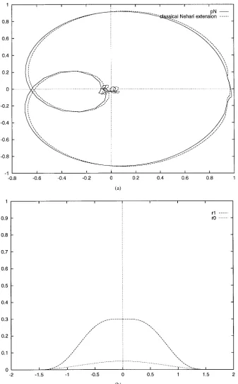
[image:7.612.133.470.53.595.2](b) Fig. 1. (a) dist(pN; H1) = 0:0236 and (b) the gauge functions r0 and r1 onJ.
function whoselog-modulus is -Lipschitz in the neighborhood of some point is itself-Lipschitz at this point. This is the local version of 2) of Lemma 2.1, and it is proved in the same manner except that we must appeal, this time, to a local version of the regularity theorem for conjugate functions (see the proof of [7, III, Corollary 1.4]). To circumvent the discontinuity problem ate6ia, we introduce another Nehari problem, equivalent to (19). Letp be the first-order trigonometric polynomial which coincides withpN ate6ia so that
(pN0 p)w1=;1=("+r)is continuous on . The Nehari problem
min
g2H k(pN0 p)w1=;1=("+r)0 gk1 (25)
is clearly equivalent to (19) under the transformation v = g +
pw1=;1=("+r) and consequently assumes the same value. The
di-chotomy procedures described before may now be performed numer-ically by solving (25) iteratively, and this was done in the example presented in Section III.
Proof of Theorem 2.2: We are given that the points (zk) and
(z0
k) are the th roots of unity for some integer . We take here h
to be the functionef(e )defined by (6). The approximate valuesbk
of h on J will be taken to be ea (zk0). This choice is mainly for
(a)
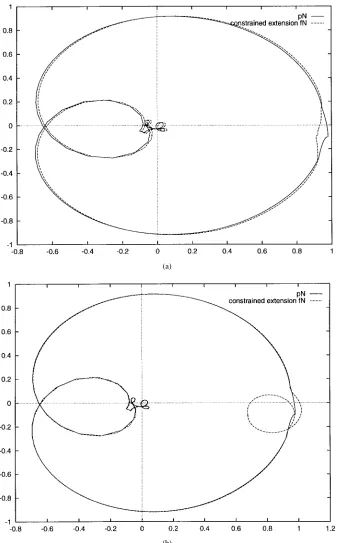
[image:8.612.133.471.53.596.2](b)
Fig. 2. (a) gauge function r0; 1 = 0:0122, and (b) gauge function r1; 1 = 0:003 28.
To construct the trigonometric polynomial pN we use the noisy values (ak)Nk=0N of f on I together with the values (bk) on J
to produce the discrete de la Vall´ee–Poussin polynomialVs; with
4s+1, as in [11]. Because = max fjak0f(zk)j; jbk0h(z0k)jg,
this is equivalent to using measurements of ^f = f _ h with an error of at most and hence (see [11, Th. 3.1]):
k ^f 0 pNk1 (4 + 2=s)(dist( ^f; Ps) + ):
Nowdist ( ^f; Ps) 32!f^(=s+1) by Jackson’s theorem [16], which,
given the definition of ^f, implies that (10) holds. One could improve
upon this bound by considering a smoother extension ^f to f. One way to do this would be to chooseh to be a function cubic (in ) which matchesf and its derivatives at the points z6N(this, of course, assumes one is able to estimate these derivatives). To get the (bk), one could use in this case a cubic polynomial matching the noisy values a6(N01) and a6N, as in [14].
Recall now that the final modelfNis the solution to the extremal problem (17). Moreover, by the proof of Lemma 2.1, we see that
error in the identified modelfN:
kf 0 fNkI;1 kf 0 pNkI;1+ kpN0 fNkI;1 2k ^f 0 pNk1
and on J
jh 0 fNj jh 0 pNj + jpN0 fNj
kh 0 pNkJ;1+ (r + 1(N)) r + 2k ^f 0 pNk1:
III. NUMERICALEXAMPLES
Our main example consists of real data measured on a hyper-frequencies filter of the CNES. The bandwidth I is defined by
a = =2, and we are given 801 noisy pointwise values (ak), so
thatN = 400. We first complete these data outside the bandwidth by rough estimates, and we construct the trigonometric polynomialpN
using discrete de la Vall´ee–Poussin polynomials. Fig. 1(a) shows the result of the classical Nehari extension topN, which gives rise to an error of value 0.0236 inL1( ). We then compute the solution fNto the constrained approximation problem associated topNfor different gauge functionsr until an acceptable tradeoff is found between 1 andr; these gauge functions are plotted in Fig. 1(b). If no satisfactory compromise can be found, one can change the reference behavior on
J, using the previous computations, in order to make a more accurate
choice. The corresponding results are shown in Fig. 2(a) and (b). We have also considered the function f(z) = 3(z2+ 1)=(z2+
2z + 5), already studied (using information on the whole circle) in
[8], [11], and [12]. Full details can be found in [3]. IV. CONCLUSION
In this paper, we presented a framework for robust band-limited identification which extends the existing one for robust identification on the whole axis (or circle) that was introduced in [9]. We also developed a constructive algorithm to perform such a band-limited identification, which recovers the transfer-function on the bandwidth in a robust fashion while meeting gauge constraints at the remaining frequencies. The procedure is very similar in spirit to the two-stage algorithms proposed in [8], [9], [11], and [12] but appeals to a bounded extremal problem which may be seen as a generalization of the classical Nehari problem. We also derived error bounds in a standard case and presented examples on real data.
There are at least two further questions which, in our opinion, deserve further study. The first arises from the observation that the identification procedure can be applied to any sequence of data a0; a1; 1 1 1 ; b1; b2; 1 1 1; the question is: “What is the limit
behavior of Tr; N; M(a0; 1 1 1 ; aN; b1; 1 1 1 ; bM) if the data do
not converge (pointwise in l1) to some interpolation sequence
f(a0); f(a1); 1 1 1 ; h(b1); h(b2); 1 1 1 with f 2 A( ), f _ h 2 C( ),
andjf 0 hj r on J?” The second question stems from the fact that our identification scheme converges uniformly tof on I but only weak–3 to f on J. This is enough to recover f uniformly on compact subsets of the half-plane (or of the disk) by the Poisson formula but not to recover f itself. Now, still assuming (3), what additional hypotheses would be needed onf in order to design an algorithm producing some stronger type of convergence? We think both questions are important in connection with the practical value of such schemes.
REFERENCES
[1] E. W. Bai and S. Raman, “A linear interpolatory algorithm for robust system identification with corrupted measurement data,” IEEE Trans.
Automat. Contr., vol. 38, pp. 1236–1241, 1993.
[2] L. Baratchart, J. Leblond, and J. R. Partington, “Hardy approximation toL1functions on subsets of the circle,” Constructive Approximation, vol. 12, no. 3, pp. 423–436, 1996.
[3] L. Baratchart, J. Leblond, J. R. Partington, and N. Torkhani, “Robust identification in the disc algebra from band-limited data,” INRIA Res.
Rep., no. 2488, 1995.
[4] T. Basar and P. Bernhard,H1-Optimal Control and Related Minimax Design Problems, A Dynamic Game Approach. Boston: Birkh¨auser, 1991.
[5] B. Francis, A Course InH1 Control Theory, LNCIS. New York: Springer-Verlag, 1987.
[6] J. H. Friedman and P. P. Khargonekar, “Application of identification in H1to lightly damped systems: Two case studies,” IEEE Trans. Contr.
Syst. Tech., vol. 3, pp. 279–289, 1995.
[7] J. B. Garnett, Bounded Analytic Functions. New York: Academic, 1981.
[8] G. Gu and P. P. Khargonekar, “Linear and nonlinear algorithms for identification inH1with error bounds,” IEEE Trans. Automat. Contr., vol. 37, pp. 953–963, 1992.
[9] A. J. Helmicki, C. A. Jacobson, and C. N. Nett, “Control-oriented system identification: A worst-case/deterministic approach in H1,”
IEEE Trans. Automat. Contr., vol. 36, pp. 1163–1176, 1991.
[10] K. Hoffman, Banach Spaces of Analytic Functions. New York: Dover, 1988.
[11] J. R. Partington, “Robust identification and interpolation inH1,” Int.
J. Contr., vol. 54, pp. 1281–1290, 1991.
[12] , “Robust identification in H1,” J. Math. Anal. Appl., vol. 166, pp. 428–441, 1992.
[13] , “Algorithms for identification in H1 with nonequally spaced function measurements,” Int. J. Contr., vol. 58, pp. 21–31, 1993. [14] , “Interpolation in normed spaces from the values of linear
func-tionals,” Bull. London Math. Soc., vol. 26, pp. 165–170, 1994. [15] V. V. Peller, “Hankel operators and continuity properties of best
approximation operators,” Algebra i Analiz., vol. 2, pp. 162–190, 1990. [16] M. J. D. Powell, Approximation Theory and Methods. Cambridge:
Cambridge Univ. Press, 1981.
[17] N. P. Rubin and D. J. N. Limebeer, “H1identification for robust con-trol,” in Proc. Amer. Contr. Conf., Baltimore, MD, 1994, pp. 2040–2044. [18] N. Torkhani, “Robust interpolation and approximation for disc algebra functions on subsets of the circle,” J. Comput. Appl. Math., to be published.
[19] N. J. Young, An Introduction to Hilbert Space. Cambridge: Cambridge Univ. Press, 1988.