Extracting Boolean rules from CA patterns

White Rose Research Online URL for this paper:

http://eprints.whiterose.ac.uk/796/

Article:

Yang, Y.X. and Billings, S.A. (2000) Extracting Boolean rules from CA patterns. IEEE

Transactions on Systems Management and Cybernetics Part B: Cybernetics, 30 (4). pp.

573-581. ISSN 1083-4419

https://doi.org/10.1109/3477.865174

eprints@whiterose.ac.uk

https://eprints.whiterose.ac.uk/

Reuse

Unless indicated otherwise, fulltext items are protected by copyright with all rights reserved. The copyright

exception in section 29 of the Copyright, Designs and Patents Act 1988 allows the making of a single copy

solely for the purpose of non-commercial research or private study within the limits of fair dealing. The

publisher or other rights-holder may allow further reproduction and re-use of this version - refer to the White

Rose Research Online record for this item. Where records identify the publisher as the copyright holder,

users can verify any specific terms of use on the publisher’s website.

Takedown

If you consider content in White Rose Research Online to be in breach of UK law, please notify us by

Correspondence

Extracting Boolean Rules from CA Patterns

Yingxu Yang and S. A. Billings

Abstract—A multiobjective genetic algorithm (GA) is introduced to

iden-tify both the neighborhood and the rule set in the form of a parsimonious Boolean expression for both one- and two-dimensional cellular automata (CA). Simulation results illustrate that the new algorithm performs well even when the patterns are corrupted by static and dynamic noise.

Index Terms—Boolean identification, cellular automata, genetic

algo-rithms, spatio-temporal systems.

I. INTRODUCTION

Cellular automata (CA) are mathematical models for complex nat-ural systems containing large numbers of simple identical components with local interactions. Since the pioneering work of John von Neu-mann during the 1950s [1], cellular automata have been largely em-ployed as a modeling class to approximate nonlinear discrete and con-tinuous dynamical systems in a wide range of applications [2]–[5]. However the inverse problem of determining the CA that satisfies gen-eral sets of prespecified constraints [6] has received relatively little at-tention. One of the most essential problems in this case is the identi-fication of CA, i.e., how to learn the underlying rule that governs the local behavior of cells from temporal slices of the global evolution of the spatio-temporal pattern.

CA in the classical sense are autonomous systems, i.e., there are no external inputs exerting an influence on the evolution. It is only pos-sible to observe the evolution of CA as a series of snapshots of the global states at various times in a certain finite interval of the evo-lution. An identification procedure can then be established based on using these fixed global states. In CA identification, it is assumed that a given spatio-temporal pattern (a pattern that evolves in both space and time) has a dimension d (d 1) and can be described by a cellular automaton. Identification of a CA involves determining a min-imal description of the CA3 that precisely simulates such that the size of the neighborhood of3 is as small as possible. It is therefore necessary to determine not only the CA rule but also the structure of the CA neighborhood. Ideally, the identification technique should pro-duce a concise expression of the CA rule. This ensures that the model is parsimonious and can be readily interpreted for hardware realization of the cellular automaton. Richards et al. [7] proposed a method for ex-tracting CA rules from given spatio-temporal patterns using a genetic algorithm (GA). Adamatskii [8] discussed the complexity of identifi-cation of cellular automata and presented sequential and parallel al-gorithms for computing the local transition table. However, neither of these authors obtained a clear neighborhood structure or parsimonious rule expression.

In digital circuit design [9]–[14], small Boolean expressions are searched to reproduce given data tables. But these solutions are

Manuscript received July 10, 1998; revised February 14, 1999 and April 23, 2000. This work was supported by the University of Sheffield and U.K. EPSRC. This paper was recommended by Associate Editor J. Oomen.

The authors are with the Department of Automatic Control and Systems Engineering, University of Sheffield, Sheffield S1 3JD, U.K. (e-mail: yingxu@acse.shef.ac.uk; s.billings@sheffield.ac.uk).

Publisher Item Identifier S 1083-4419(00)06717-0.

concerned with minimizing known Boolean functions and do not address the general problem of determining the CA rule from an observed possibly noisy complex multidimensional pattern. The latter problems are much more complex, as discussed by Richards et al. [7], and a solution would offer an important step forward in the modeling of spatially extended systems that arise in such diverse fields as pattern formation, fluidic mixing, brain imaging and in data compression problems.

This paper considers the identification of Boolean expressions for one–dimensional (1-D) and two–dimensional (2-D) CA. An evolutionary algorithm is proposed using a multiobjective genetic algorithm to extract a precise local Boolean expression of the CA rule from given spatio-temporal patterns blurred by noise. The remainder of the paper is organized as follows. In Section II, the definition of a group of 1-D and 2-D CA is introduced. Section III reformulates the Boolean expression for 1-D CA rules and extends these to the 2-D case. The GA search for Boolean expressions of CA rules is then presented with an emphasis on the construction of parsimonious forms of CA rules. Simulation results are contained in Section IV, and Section V discusses the efficiency of the algorithm.

II. ONE-ANDTWO-DIMENSIONALCELLULARAUTOMATA

A cellular automaton is composed of three parts: a discrete lattice, a neighborhood and a rule for local transitions. Attention in this paper is restricted to binary CA where the cells can only take binary values.

A. Neighborhoods

The neighborhood of a cell is the set of all the cells capable of directly influencing the evolution. Sometimes this includes the cell itself. The neighborhoods shown in Fig. 1 are used often and have proper names. CA neighborhoods can take cells from various spatial and temporal scales. For simplicity, this paper only considers neighborhoods com-posed of cells from time stept 0 1, but the results are not restricted to this case.

B. Local Rules

The local transition rule updates all cells synchronously by assigning to each cell, at a given time step, a value which depends only on the neighborhood. The most common method to define the local transition rule is to use a transition table analogous to a truth table. In this truth table, the rule is labeled by assigning neighborhoods in ascending nu-merical order and specifying which neighborhoods map to zero and which to one. The truth table is also called the component form of the CA rule. The component form of a three-site 1-D ruleR is shown as follows:

000 001 010 011 100 101 110 111 r0 r1 r2 r3 r4 r5 r6 r7

20 ₂1 ₂2 ₂3 ₂4 ₂5 ₂6 ₂7

where the first row gives all the possible states the cells within the neighborhood could take. The ri’s in the second row are the rule components which can take only binary numbers with 1’s indicating that the components are included in the rule and 0’s indicating otherwise. The last row shows the coefficients associated with the corresponding components. The rule R can be defined as

Fig. 1. Examples of most frequently used 1-D and 2-D neighborhoods. (a) 1-D von Neumann neighborhood. (b) 2-D von Neumann neighborhood. (c) 2-D Moore neighborhood.

R = (r0; r1; r2; r3; r4; r5; r6; r7). The numerical label D assigned to R is given by D(R) = 2 01_s=0 rs2s, which is simply the sum of the coefficients associated with all nonzero components. All this applies to the ruleR with any three-site neighborhoods irrespective of the neighborhood structures. For example, a very often used 1-D three-site ruleRule22 is defined as Rule22 = (01 101 000) and the numerical labelD(Rule22) = 21+ 22+ 24= 22.

III. EXTRACTINGBOOLEANRULESUSINGGENETICALGORITHMS

A. Boolean Form of CA Rules

For a 2-D CA, the local transition can be denoted assnew(i; j) =

flt(NN(i; j)), where sN new(i; j) is the updated state of cell(i; j) at time stept and NNN(i; j) represents the states of the cells within the neigh-borhood ofcell(i; j) at time step t 0 1. Reducing the dimensions in this expression will yield models for 1-D CA as a special case. The local transition functionflt is equivalent to the local transition table of length2n, wheren is the size of the neighborhood. Therefore, flt can be viewed as a Boolean function ofn variables, and CA rules can be expressed as Boolean rules. There are two different ways of con-structing Boolean rules, using NOT, AND, OR, and NOT, AND, XOR logical operators, respectively. This paper only considers the latter for-mulation because this usually involves fewer logical operations than the former formulation for the same rule. For example, the Boolean form of Rule22 = (01 101 000), which is illustrated in Table I, is

snew(j) = C 8 D. For all n-site 1-D CA rules, there is a simple pro-cedure for the construction of the Boolean expression in terms of NOT,

AND and XOR operators given the component form (see [15],

Algo-rithm 1.1, p. 30 for details). The NOT operator can be removed from the obtained Boolean expression by applyingNOT(a) = 1 8 a. Fur-thermore, applying0 8 a = a and (a 8 b) 3 c = a 3 c 8 b 3 c, it is then straightforward to state, e.g., that all the 1-D three-site binary CA can be represented by a Boolean function with only AND and XOR operators of the form

snew(j) = a08 a1s(j 0 1) 8 a2s(j) 8 a3s(j + 1)

8 a4(s(j 0 1) 3 s(j)) 8 a5(s(j) 3 s(j + 1))

8 a6(s(j 0 1) 3 s(j + 1))

8 a7(s(j 0 1) 3 s(j) 3 s(j + 1)) (1) whereai(i = 0; 1 1 1 ; 7) are binary numbers and ai= 1 indicates that the following term is included in the Boolean function whileai = 0 indicates that the following term is not included. Note that the number of possible expressions in (1) is28= 256, which is exactly the number of all three-site 1-D rules. This implies that the representation in (1) is unique: one set offai; i = 0; 1 1 1 ; 7g corresponds to one and only one CA rule.

TABLE I

THEBOOLEANFORM OFRule22 USINGNOT, AND,ANDXOR OPERATORS.

B = s(j 01)8s(j), C = B 8s(j +1), D = s(j 01)3s(j)3s(j +1)—3,

AND8 REPRESENT THEANDANDXOR OPERATOR, RESPECTIVELY

This can be extended to multidimensional CA. For example any 2-D CA with a five-site von Neumann neighborhood can be represented by a Boolean expression:

snew(i; j) = a08 a1s(i 0 1; j) 8 1 1 1

8 a31(s(i 0 1; j) 3 1 1 1 3 s(i + 1; j)): (2) Extending this further, every CA with an n-site neighborhood

fcell(x1); 1 1 1 ; cell(xn)g may be written as

snew(xj) = a08 a1s(x1) 8 1 1 1 8 aP(s(x1) 3 1 1 1 3 s(xn)) (3)

whereP = 2n0 1 and cell(xj) is the cell to be updated.

B. Extracting Boolean Rules using a Genetic Algorithm

Equation (3) is important because it significantly reduces the com-plexity of CA identification by using a reduced set of logical opera-tors and candidate terms. The difficulty in identifying multidimensional CA is also decreased because higher-dimensional CA rules are reduced to an equation which depends on the size of the neighborhood rather than the dimensionality. Assume that the only a priori knowledge is the dimension of the CA, which can be obtained from examining the spatio-temporal patterns [7]. Then the emerging difficulty lies in how to determine which terms should be included in the Boolean expres-sion and which should be discarded. The problem is very similar to the term selection problem in structure detection for nonlinear system identification [16]. However, in CA identification all the terms are com-bined by the XOR operator and are therefore nonlinear-in-the-parame-ters, whereas in nonlinear system identification all the items are com-bined by the ordinary addition operator and can often be configured to be linear-in-the-parameters. This difference increases the difficulty of the CA term selection problem.

Note that CA term selection is different from and more difficult than Boolean function minimization for which many useful techniques are available, especially in the digital circuit design literature [9]–[14]. CA term selection involves both identifying and minimizing Boolean func-tions while methods related to Boolean function minimization usually only consider deriving the equivalent minimum expression from al-ready known Boolean functions. The identification is difficult because of the logical terms, particularly when cellular automata with large size neighborhoods and, therefore, a large number of candidate log-ical terms, are involved.

In the present study, this problem is solved by evolving a genetic algorithm [17], [18] in the search for appropriate terms through the space of logical models constructed upon AND and XOR operators. This algorithm is implemented as follows.

1) Population: In the current application, each candidate Boolean

as a1 2 (P + 1) binary vector ci, whereP = 2n0 1 and n is the size of the largest neighborhood under consideration. Each entry in theith chromosome corresponds to a term in the following term set:

ci(1) ! 1; ci(2) ! s(x1); 1 1 1 ; ci(n + 1) ! s(xn);

ci(n + 2) ! s(x1) 3 s(x2); 1 1 1 ;

ci(P + 1) ! s(x1) 3 1 1 1 3 s(xn)

wherec_i(j) = 1 indicates that the associated term has been selected andci(j) = 0 indicates otherwise. Define

f = [1 s(x1) 1 1 1 s(x1) 3 1 1 1 3 s(xn)] C = [c1 1 1 1 cnp]

wherenp is the number of chromosomes in the population.

2) Multiobjective Fitness Function: The fitness function is

de-signed to measure the performance of Boolean rules represented by the chromosomes in regenerating the observed spatio-temporal patterns. Before introducing the fitness function for the CA term selection problem, the vector XOR operator8 is defined as follows:

[ a1 1 1 1 an] 8 [ b1 1 1 1 bn]T

= (a13 b1) 8 1 1 1 8 (an3 bn)

where3 denotes the AND operator. For example,

[ a1 0 a3] 8 [ b1 b2 b3]T

= (a13 b1) 8 (0 3 b2) 8 (a33 b3) = (a13 b1) 8 (a33 b3):

In the present problem, an important measure of the performance of the chromosomes is the modulus of errors function defined as

Mer(i) =

SET

r

jy(i; j) 0 ^y(i; j)j (4) where

r number of data points in the data set extracted from the CA patterns;

y(i; j) measured state at data pointj for chromosome

i;

^y(i; j) = ci8 fj predicted state.

IfMer is chosen as the fitness function, a solution with the least mod-ulus of errors will be found. However, it is not guaranteed that the asso-ciated neighborhood is correct and minimal. This is because there may be more than one model that produces a minimumMer. The initial as-sumed neighborhood almost always encompasses more cells than are actually in the real neighborhood. A 1-D ruleRule30 with a von Neu-mann neighborhood, for example, is most concisely represented as

snew(j) = s(j 0 1) 8 s(j) 8 s(j + 1) 8 (s(j) 3 s(j + 1)) (5)

while during the search for this rule the candidate rules are often searched for over a larger neighborhood. For example, candidate rules can be assumed to be operating on a five-site neighborhood

fcell(j 0 2); cell(j 0 1); cell(j); cell(j + 1); cell(j + 2)g and of

the form

snew(j) = a08 a1s(j 0 2) 8 1 1 1

8 a31(s(j 0 2) 3 1 1 1 3 s(j + 2)): (6) It is highly likely that more than one expression including (5) may be selected from (6) to match the patterns. The solution is therefore not necessarily unique, and this often leads to a false extension of the neighborhood.

Note that a rule with a larger neighborhood cannot be represented by a rule with a smaller neighborhood while a rule with a smaller

neigh-borhood can often be expressed by a rule with a larger neighneigh-borhood. Therefore, the best model is always the smallest model amongst all the possible models chosen. This is the principle of parsimony. Thus, another search objective must be added to direct the algorithm to pro-duce a parsimonious logical model with minimal modulus of errors. An efficient approach to accommodate the second search objective is to employ a multiobjective fitness function. In the present study, the two search objectives are to minimizeMer and to minimize the number of terms in all models with the sameMer. The multiobjective fitness function in this study is based on a ranking scheme according to the concept of Pareto optimality [17]. This will guarantee equal probability of reproduction to all nondominant chromosomes and should generate a solution nearest to the optimal. The multiobjective fitness function is constructed as follows.

a) Each chromosome in the current population is ranked with re-spect toMer. The chromosome with the least Mer occupies the first position, the chromosome with the second leastMer occupies the second position and so on. Chromosomes with the same error share the same rank. So

RANK 1 1 1 1 i i

ERROR Mer(1) 1 1 1 Mer(i) Mer(i + 1)

RANK i 1 1 1 np

ERROR Mer(i + 2) 1 1 1 Mer(np)

with

Mer(1) < 1 1 1 < Mer(i) = Mer(i + 1) = Mer(i + 2) < 1 1 1 < Mer(np):

b) Define the structure function St(i) for the ith chromosome as St(i) = P +1_j ci(j). Resort the orders of chromosomes sharing the same rank in proportion to the associatedSt(i) and keep the ranking of the remainder unchanged. Thus

RANK 1 1 1 1 i i + 1

ERROR Mer(1) 1 1 1 Mer(i) Mer(i + 1) STRUCTURE St(1) 1 1 1 St(i) St(i + 1)

RANK i + 1 1 1 1 np

ERROR Mer(i + 2) 1 1 1 Mer(np) STRUCTURE St(i + 2) 1 1 1 St(np)

with

St(1) < 1 1 1 < St(i) < St(i + 1) = St(i + 2) < 1 1 1 < St(np):

c) The multiobjective fitness function of theith chromosome is fi-nally defined as

fit(i) = _{MAX(rank(i)) 0 MIN(rank(i))}MAX(rank(i)) 0 rank(i) : (7) The ranking technique results in a search with a preference toward min-imizingMer. The structure function St will not have any impact on the first few steps of the search and the fitness of each chromosome in those steps is determined exclusively byMer because all the chromo-somes are highly likely to hold various ranks at that initial stage. Only after certain chromosomes have converged to a similarMer is it pos-sible to rearrange the ranking at thatMer according to the associated

St. This search is therefore able to always select chromosomes with the

minimum structure within the span of the lowestMer. Hence, chro-mosomes with a parsimonious logical expression and minimum error will remain in the latest population to yield the final solution.

(a) (b)

(c) (d)

Fig. 2. Noise-free pattern and static noise contaminated patterns produced by 1-DRule22. (a) p = 0. (b) p = 0:05. (c) p = 0:1. (d) p = 0:2.

different search objectives of minimizingMer and St, respectively. Each candidate in the main population is produced by genetic commu-nication between the two subpopulations and is subject to evaluation by the ranking technique.

For details of reproduction, crossover, and mutation see [18] and [20].

3) Summary of the CA Term Selection Algorithm: The CA term

se-lection algorithm can be summarized as follows.

a) Generate three initial population setsP, Q and R with each consisting ofnp individuals. Set the current generation number

i = 1.

b) ComputeMer for each individual in P. Calculate St in each chromosome inQ. Rank the individuals in R using the ranking technique. Calculate the fitness value.

c) Apply the parent selection technique toP and Q.

d) Employ crossover and mutation toP and Q separately to produce the corresponding offspring setsP0 andQ0. Employ crossover and mutation toP and Q combined to produce the offspring set

R0_{for the population setR .}

e) Calculate the corresponding fitness values for the chromosomes in the offspring setsP0,Q0andR0. Select thenp fittest individ-uals from both the population setsP, Q, and R and the corre-sponding offspring setsP0,Q0 andR0, respectively, by com-paring the fitness values. ResetP, Q, and R using the cor-responding newly selectednp individuals. Set the generation numberi = i + 1 and nullify the three offspring sets P0,Q0 andR0.

f) Return to c) and repeat until a prespecified number of generations has been reached.

IV. SIMULATIONANALYSIS

A. The Effects of Noise

In cellular automata, noise is a form of imperfection which at a crit-ical magnitude is able to induce an essential phase transition that can suddenly change the behavior of the CA. Static noise can be added to a spatio-temporal pattern by first evolving a deterministic CA rule and then randomly flipping a limited number of binary values according to a specified probabilityp, where p = q1=q2,q1is the number of cells to be flipped, andq2is the total number of cells in the spatio-temporal pattern. This is referred to as static noise because it is added after the CA evolution. Fig. 2 shows the noise-free pattern (p = 0) for the 1-D

Rule22 with von Neumann neighborhood and the same pattern

cor-rupted by noise with probabilities of switchingp = 0:05, p = 0:1, and

p = 0:2, respectively. All these were developed on a 200 2 200 lattice

with time evolution from top to bottom, and with a periodic boundary condition, i.e., the lattice is taken as a circle in the horizontal dimen-sion, so the first and last sites are identified as if they lay on a circle of finite radius. The evolution started from an initial condition of a ran-domly generated binary vector.

(a) (b)

(c) (d)

(e) (f)

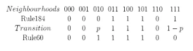
Fig. 3. The transition fromRule184 (p = 0) to Rule60 (p = 1) with p varying to indicate different noise densities (a) p = 0, (b) p = 0:1, (c) p = 0:5, (d)

p = 0:65, (e) p = 0:8 and (f) p = 1:0.

under the transition rule in Table II. Note that the maximum noise den-sity for the transition is 0.5. For example, whenp = 0:6, the transition behaves more likeRule60 than Rule184 and, therefore, the noise den-sity for the transition should be considered as1 0 p = 0:4 for Rule60 rather than 0.6 forRule184.

B. Extracting Boolean Rules from 1-D CA Patterns

1) From Patterns Corrupted by Static Noise: Assume the

neighbor-hood structure of a class of 1-D CA is defined byfcell(j02); cell(j0

1); cell(j); cell(j + 1); cell(j + 2)g. Given the spatio-temporal

pat-terns in Fig. 2, the CA term selection algorithm was used to produce the results in Table III. A typical run using data extracted from the noise-free pattern in Fig. 2(a) is shown in Fig. 4. In each case, 100 trials were conducted using different initial assignments. The program was terminated after 120 generations had been reached. Except for method

TABLE II

TRANSITIONRULE FROMRule184TORule60 WHERE0 < p < 1

a with p = 0, the optimal solutions were found in all the 100 trials. It

TABLE III

SUMMARY OFRESULTSOBTAINED INEXTRACTINGRule22 FROM THE PATTERNS INFIG. 2,USINGMETHODa: ANUNMODIFIEDGENETICALGORITHM

WITHMerAS THEFITNESSFUNCTION,ANDMETHODb: THECA TERM SELECTIONALGORITHM. THE“GENERATIONS” COLUMNINDICATES THE NUMBER OFGENERATIONSREACHED WHEN THEOPTIMALSOLUTION WAS FOUND. AV.R.T. REPRESENTS THEAVERAGERUNTIME IN THESEARCH FOR THEOPTIMALSOLUTION INONETRIAL. ONEHUNDREDTRIALS WEREMADE

FOREACHPROBLEM. THEOPTIMALSOLUTION ISALREADYKNOWN

with different trials, but all involved an incorrectly extended neigh-borhood. For example, the rule produced from the evolution shown in Fig. 4(a) is

snew(j) = s(j 0 1) 8 s(j) 8 s(j + 1) 8 (s(j 0 1) 3 s(j + 1))

8 (s(j 0 1) 3 s(j) 3 s(j + 2)) 8 (s(j 0 1) 3 s(j + 1) 3 s(j 0 2)) 8 (s(j 0 1) 3 s(j + 1) 3 s(j + 2)) 8 (s(j 0 1) 3 s(j) 3 s(j + 1) 3 s(j 0 2)) 8 (s(j 0 1) 3 s(j) 3 s(j 0 2) 3 s(j + 2))

8 (s(j 0 1) 3 s(j + 1) 3 s(j 0 2) 3 s(j + 2)): (8) In contrast, whenp = 0 method b generated only one Boolean rule in all 100 trials, this Boolean rule is

snew(j) = s(j01)8s(j)8s(j+1)8(s(j01)3s(j)3s(j+1)): (9)

Although the Boolean rules in both (8) and (9) produce the same cor-rect truth table ofRule22, the former covers a five-site neighborhood

fcell(j 0 2); cell(j 0 1); cell(j); cell(j + 1); cell(j + 2)g while

the real neighborhood should befcell(j 0 1), cell(j), cell(j + 1)g. The neighborhood structure of the former is therefore suboptimal. This result was obtained because methoda selected the rules with the min-imumMer without considering the structure of the neighborhood. In contrast, the Boolean rule in (9) was obtained using a search also taking into account the number of terms in the candidate rule, and this pro-duced a rule exactly the same as listed in [15] with a correct neighbor-hood and a parsimonious Boolean expression. This is also illustrated in Fig. 4(b) whereSt diminishes after Mer has settled on zero. Further-more, the modulus of errors using methodb converged considerably faster than using methoda because in method b, subpopulations were incorporated to accelerate the convergence. This effect is demonstrated in Table III, where the average run-time using methodb was almost half the time using methoda. It can also be seen from Table III that althoughMer did not converge to zero for either p = 0:1 or p = 0:2, due to random flipping of some cell values, the correct and parsimo-nious Boolean expression in (9) was still obtained in both cases. This suggests that the CA term selection algorithm is not sensitive to static noise when the noise density is within a certain amplitude, in this case,

p 0:2.

2) From Patterns Corrupted by Dynamic Noise: Dynamic noise is

immediately involved in the CA evolution and can considerably

af-(a)

(b)

Fig. 4. Search process forRule22 using the noise-free pattern, and methods

a and b, respectively, (a) using method a and (b) using method b. Legend: The

dashed line is the evolution of the number of terms in the chromosome with the best fitness. The solid line is the evolution of the modulus of error of the chromosome with the best fitness.

TABLE IV

SUMMARY OFRESULTSOBTAINED INEVOLVING THETRANSITION FORM

Rule184TORule60USING THECA TERMSELECTIONALGORITHM

snew(j) = s(j 0 1) 8 (s(j 0 1) 3 s(j)) 8 (s(j) 3 s(j + 1)), which is exactly the same as the Boolean form ofRule184 listed in [15]. The result in Table IV forp = 0:1 produces

snew(j) = s(j 0 1) 8 (s(j 0 1) 3 s(j))

8 (s(j) 3 s(j + 1)) 8 (s(j 0 1) 3 s(j) 3 s(j + 1))

which generates the rule components (01 011 100). Note that in com-parison with the correct rule components forRule184 (01 011 101), the last bit in the identified rule components is incorrect. The reason for this appears to lie in the nature of the rule itself. Rules that pro-duce simple patterns of self-repetition or shifting imply that a certain number of combinations of the states of the cells within the neighbor-hood have probably never appeared in the existing data set. Hence, the search is unlikely to learn that particular behavior and most probably in-discriminately selects a rule from a range of rules satisfying only other combinations. ForRule184, even though the evolution is slightly com-plicated, and the data set extracted from the noise-free pattern is rich enough to allow the identification of the correct rule (00 011 101), the combination of the states of the cells within the neighborhood (111), which corresponds to the last component, appears infrequently and the noise simplifies the data set by eliminating (111). Subsequently, the search failed to learn the behavior of (111) and, hence, produced a wrong result. A similar phenomena appears in other simple 1-D rules such asRule46, Rule116, Rule72, and Rule172. The search may re-peatedly produce incorrect rules even after the size of the data set has been enlarged. Consequently, under certain combination of rules and initial conditions, the optimal solution can be deduced only provided sufficient data are available.

However, forp = 0:8, where the noise density is 1 0 0:8 = 0:2 for the rule transition, the search result issnew(j) = s(j 01)8s(j). This result is correct and parsimonious and exactly the same as the Boolean expression forRule60 listed in [15], even though the noise level is 10% higher than inp = 0:1. This appears to be because of the chaotic nature ofRule60, which is able to generate patterns complicated enough so that even after the patterns are contaminated by a relatively high density of noise, the data set still contains sufficient information to correctly characterize the behavior. Whenp = 1, the result is snew(j) = s(j 0

1) 8 s(j), which is the same as for p = 0:8 and is the parsimonious

Boolean expression forRule60. Note that for p = 0:65, the search also converged to the correct results(j) = s(j 0 1) 8 s(j) despite the high noise density of1 0 0:65 = 0:35 for Rule60.

The search result for the transition rule atp = 0:8 is also shown in Table V. Although the data were contaminated by a dynamic noise with density1 0 0:8 = 0:2, which had substantial impact on the growing patterns (the growth of the noise corrupted patterns was 100% faster than the noise-free patterns), and the error did not converge to zero, the search produced the same correct and parsimonious Boolean rule as identified in the noise-free case (p = 1). This suggests that the CA term selection algorithm is robust in the presence of dynamic noise even for the 2-D case.

C. Extracting Boolean Rules from 2-D CA Patterns

Table V shows the results of the search for CA rules using data produced by both the evolution of a deterministic 2-D rule

Rule(01 101 010 11 101 110 01 001 111 11 100 100) and a

transition(01 101 010 1 110 111(1 0 p) 01 001 111 p1 100 100) of the same rule atp = 0:8 over the five-site von Neumann neigh-borhood in Fig. 1(b). The neighneigh-borhood was initially assumed as the nine-site Moore neighborhood in Fig. 1(c). In each case, 100 trials were conducted using different initial assignments. The program was terminated when 800 generations had been reached. The result

TABLE V

SUMMARY OFRESULTSOBTAINED INEXTRACTING A2-D CA RULE AND THE SAMERULECORRUPTED BY ADYNAMICNOISE/INTRANSITION ATp = 0:8

USING THECA TERMSELECTIONALGORITHM

in Table V for p = 1 produces a Boolean expression of the XOR combination of the following 20 terms:

B = s(i; j 0 1); C = s(i; j) D = s(i; j + 1); E = s(i 0 1; j) F = s(i + 1; j) 3 s(i; j + 1) G = s(i; j 0 1) 3 s(i; j) H = s(i; j 0 1) 3 s(i; j + 1)

I = s(i; j 0 1) 3 s(i + 1; j) J = s(i; j) 3 s(i; j + 1)

K = s(i + 1; j) 3 s(i; j 0 1) 3 s(i; j) L = s(i + 1; j) 3 s(i; j 0 1) 3 s(i; j + 1) M = s(i + 1; j) 3 s(i; j) 3 s(i; j + 1)

N = s(i + 1; j) 3 s(i; j) 3 s(i 0 1; j) O = s(i + 1; j) 3 s(i; j + 1) 3 s(i 0 1; j) P = s(i; j 0 1) 3 s(i; j) 3 s(i; j + 1) Q = s(i; j) 3 s(i; j + 1) 3 s(i 0 1; j)

R = s(i + 1; j) 3 s(i; j 0 1) 3 s(i; j) 3 s(i; j + 1) S = s(i + 1; j) 3 s(i; j 0 1) 3 s(i; j + 1) 3 s(i 0 1; j) T = s(i + 1; j) 3 s(i; j) 3 s(i; j + 1) 3 s(i 0 1; j) U = s(i + 1; j) 3 s(i; j 0 1) 3 s(i; j)

3 s(i; j + 1) 3 s(i 0 1; j):

Table VI shows the tabular form of this identified Boolean rule. It can be seen that this rule covers a five-site von Neumann neighborhood, which has been extracted from the assumed nine-site Moore neighbor-hood and is correct. The truth table produced from the identified rule is also correct. Therefore, according to the principle of parsimony, the identified Boolean rule is optimal. However as shown in Table V the average run time is much longer than in the 1-D noise-free case. This is because the growth of the size of the neighborhood will inevitably in-duce a considerable increase in the number of possible terms that can be included in the Boolean expression and, hence, an increase in the complexity of the search.

D. Extracting Boolean Rules from Patterns Produced by a Large Set of CA Rules

TABLE VI

TABULARFORM OF THEIDENTIFIED2-D BOOLEANRULE

TABLE VII

SUMMARY OFRESULTSOBTAINED INEVOLVINGSOME1-D CA RULES WITHVARIOUSSIZES OFNEIGHBORHOOD.n INDICATES THESIZE

OF THENEIGHBORHOOD

cell(j); cell(j+1), cell(j+2); cell(j+3); cell(j+4)g. The

identi-fied neighborhoods and the truth tables produced by the corresponding Boolean rules are all correct. Therefore, according to the principal of parsimony, the identified Boolean rules are all optimal.

Simulations over a large set of rules suggest that the average run time relies more on the size of the assumed neighborhood than on the size of the actual neighborhood. For example, forRule22, the average run-time in Table VII, where the initial neighborhood was assumed as nine-site, is considerably larger than in Table III, where the initial neighborhood was assumed as five-site. However, as has also been in-dicated in Table VII, under the same neighborhood assumption, rules with more cells in the actual neighborhood tend to require more gener-ations to converge to the optimal solution. Because the CA term selec-tion algorithm discriminates only the number of cells in the neighbor-hood rather than the position each individual cell occupies, the results for 2-D rules were very similar to the 1-D case and are therefore not listed in this paper.

V. CONCLUSIONS

A solution to the inverse problem in cellular automata has been pro-posed using a multiobjective evolutionary algorithm. Both 1- and 2-D cellular automata have been investigated, and it has been shown that the CA rule, in the form of a parsimonious Boolean expression, can be identified by carefully formulating the GA search procedure. The sim-ulation results illustrate the efficiency of the new algorithm and demon-strate that the correct neighborhood and CA rule can be determined in the presence of both static and dynamic noise.

REFERENCES

[1] J. von Neumann, “The general logical theory of automata,” in Cerebral

Mechanisms in Behavior—The Hixon Symposium. New York: Wiley, 1951.

[3] G. Hernandez and H. J. Herrann, “Cellular automata for elementary image enhancement,” Graph. Models Image Process., vol. 58, no. 1, pp. 82–89, 1996.

[4] S. Bhattachariee and S. Sinha, “Cellular automata based scheme for so-lution of Boolean equations,” Proc. Inst. Elect. Eng. Comput. Digital

Tech., vol. 143, no. 3, pp. 174–180, 1996.

[5] S. Surka and K. P. Valavanis, “A cellular automata model for edge re-laxation,” J. Intell. Robot. Syst., vol. 4, no. 4, pp. 379–391, 1991. [6] W. Li, N. H. Packard, and C. G. Langton, “Transition phenomena in

cellular automata rule space,” in Cellular Automata: Theory and

Exper-iment, H. Gutowitz, Ed. Cambridge, MA: MIT Press, 1991. [7] F. C. Richards, “Extracting cellular automaton rules directly from

exper-imental data,” Phys. D, vol. 45, pp. 189–202, 1990.

[8] A. I. Adamatskii, “Complexity of identification of cellular automata,”

Autom. Remote Control, pt. 2, vol. 53, no. 9, pp. 1449–1458, 1992.

[9] W. V. Quine, “A way to simplify truth functions,” Amer. Math. Monthly, vol. 62, pp. 627–631, 1955.

[10] E. J. McCluskey Jr., “Minimization of Boolean functions,” Bell Syst.

Tech. J., vol. 35, pp. 1417–1444, 1956.

[11] S. C. Gupta, “A fast procedure for finding prime implicants of a Boolean function,” Int. J. Electron., vol. 51, no. 5, pp. 701–709, 1981. [12] S. R. Perkins and T. Rhyne, “An algorithm for identifying and selecting

the prime implicants of a multiple-output Boolean function,” IEEE

Trans. Computer-Aided Design, vol. 7, pp. 1215–1218, Nov. 1988.

[13] P. P. Chu, “Applying neural networks to find the minimum cost coverage of a Boolean function,” VLSI Design, vol. 3, no. 1, pp. 13–19, 1995. [14] S. Chattopadhyay, S. Roy, and P. P. Chaudhuri, “KGPMIN: An efficient

multilevel multioutput AND-OR-XOR minimizer,” IEEE Trans.

Com-puter-Aided Design, vol. 16, pp. 257–265, Mar. 1997.

[15] B. H. Voorhees, Computational Analysis of One-dimensional Cellular Automata, ser. World Scientific Series on Nonlinear

Sci-ence. Singapore: World Scientific, 1996.

[16] S. A. Billings, S. Chen, and M. J. Korenberg, “Identification of MIMO nonlinear systems using a forward-regression orthogonal estimator,” Int.

J. Control, vol. 49, no. 6, pp. 2157–2189, 1989.

[17] Z. Michalewicz, Genetic Algorithms + Data Structures = Evolution

Pro-grams. New York: Springer-Verlag, 1994.

[18] D. E. Goldberg, Genetic Algorithms in Search, Optimization and

Ma-chine Learning. Reading, MA: Addison-Wesley, 1989.

[19] J. R. Koza, Genetic Programming: On the Programming of Computers

by Means of Natural Selection. Cambridge, MA: MIT Press, 1992. [20] A. J. Chipperfield and P. J. Fleming, “Genetic algorithms in control

sys-tems engineering,” Control Comput., vol. 23, pp. 88–94, 1996.

The Certainty Factor-Based Neural Network in Continuous Classification Domains

LiMin Fu

Abstract—The integration of certainty factors (CFs) into the neural

computing framework has resulted in a special artificial neural network known as the CFNet. This paper presents the cont-CFNet, which is devoted to classification domains where instances are described by continuous attributes. A new mathematical analysis on learning behavior, specifically linear versus nonlinear learning, is provided that can serve to explain how the cont-CFNet discovers patterns and estimates output probabilities. Its advantages in performance and speed have been demonstrated in empirical studies.

Index Terms—Certainty factor, classification, fuzzy set theory, machine

learning, neural network, probability estimation.

I. INTRODUCTION

The certainty factor (CF) model has been applied to traditional ex-pert systems for management of uncertainty [2], [17]. To map this model into a neural computing framework has generated a number of successful applications [4]–[8], [11], [13]. The term CFNet has been coined by Fu [8] to refer to an artificial neural network whose activa-tion funcactiva-tion is based on the CF model. An important result is that the CFNet can generalize more effectively than neural networks using the sigmoid activation function [7]. Recent research has shown that this network can discover the domain rules with better accuracy than the decision-tree approach [8]. Because certainty factors have traditionally been applied to rule-based environments for handling symbolic data, the CFNet has been tested in domains where instances are described by discrete nominal attributes. It would be a new challenge to apply the CFNet to domains where the data involve continuous numerical attributes. In order to realize this capability, a new system named the cont-CFNet exploits the strength of fuzzy representation. Here, a brief background on fuzzy neural networks is worthwhile.

Based on Zadeh’s fuzzy set theory [19], fuzzy logic views each pred-icate as a fuzzy set. In fuzzy logic, a linguistic variable like “size” can have several linguistic values like “small,” “medium,” or “large.” Each linguistic value is viewed as a fuzzy set associated with a membership function, which can be triangular, bell-shaped, or of another form. The degree of membership can be interpreted as the degree of possibility, which evades the requirement of satisfying the probability axioms.

The relationship between fuzzy systems and neural networks has drawn much attention since both are trainable systems capable of han-dling uncertainty and imprecision and both have found may successful applications. Their complimentary roles suggested in [10] and [14] have led to so-called fuzzy neural networks for handling the fuzzy (in-exact) nature of inference involving symbols (symbolic inference). In such networks, an input pattern is enhanced via fuzzy representation. Furthermore, when the decision function or boundary involves curves, a smooth membership function at fuzzy neural units allows close mod-eling or approximation.

Manuscript received July 11, 1999; revised May 28, 2000. This work was supported by the National Science Foundation under Grant ECS-9615909. This paper was recommended by Associate Editor W. Pedrycz.

The author is with the Department of Computer and Information Sciences, University of Florida, Gainesville, FL 32611 USA (e-mail: fu@cise.ufl.edu).

Publisher Item Identifier S 1083-4419(00)06719-4.