A new constrained total variational deblurring model and its fast algorithm

A New Constrained Total Variational Deblurring Model and Its Fast

Algorithm

Bryan Michael Williams∗_{, Ke Chen}†_{, and Simon P. Harding}‡

Abstract

Although image intensities are non-negative quantities, imposing positivity is not always sidered in restoration models due to a lack of simple and robust methods of imposing the con-straint. This paper proposes a suitable exponential type transform and applies it to the commonly-used total variation model to achieve implicitly constrained solution (positivity at its lower bound and a prescribed intensity value at the upper bound). Further to establish convergence, a convex model is proposed through a relaxation of the transformed functional. Numerical algorithms are presented to solve the resulting non-linear partial differential equations. Test results show that the proposed method is competitive when compared with existing methods in simple cases and more superior in other cases.

Key words. Total variation, image deblurring, alternating direction method of multipliers, box constraint, transforms.

AMS subject classifications. 68U10, 65J22, 65K10, 65T50, 90C25.

1

Introduction

Image processing techniques, such as image reconstruction which includes removing image noise from a given image (denoising) [29], reconstructing an image from a given blurred image (deblurring) [18], reconstructing the missing or damaged portion of an image (inpainting) [9], emphasizing the boundaries of an image by different filters or segmenting an image into subregions (segmentation) [17], have been widely used in many areas. Despite significant developments in photographic techniques and technology, blur is still a major cause for image quality degradation in clinical settings. This is due to many factors such as motion of the camera or more commonly in the case of retinal images the target scene, defocusing of the lens system, imperfections in the electronic, photographic, transmission medium, or obstructions. In this paper, we are concerned with variational models for restoration of such blurred and noisy images.

An observed blurred image can be written as a convolution of the true image with a blur function, known as the Point Spread Function (PSF) or kernel K [25]. There are three main deconvolution problems: 1) blind deconvolution, which includes the cases when both the kernel and the image are unknown [25, 26]; 2) semi-blind restoration, in which the kernel is assumed to belong to a class of parametric functions; or 3) non-blind deconvolution where only the image is unknown [18]. All three types are important not only in many scientific applications such as astronomical imaging, medical imaging, and remote sensing, but also for consumer photography.

∗_{First two authors are with Centre for Mathematical Imaging Techniques and Department of Mathematical Sciences,}

The University of Liverpool, United Kingdom. Email: [email protected]

†_{For correspondence, Email: [email protected], Web: http://www.liv.ac.uk/cmit}

Deconvolution in the case of known blur, has been investigated widely in the last few decades giving rise to a variety of solutions [2, 3, 15, 22, 27, 24, 31, 30, 33]. In non-blind deconvolution, the point spread function is assumed known even though this information is not available in most of the real applications. In many cases, we know that our restored image must have strictly non-negative intensities, but the solution by traditional methods may yield results which are not necessarily posi-tive. This has implications for most images with significant amounts of dark space, i.e. images with many pixel intensity values close to or equal to zero, as well as for blind deconvolution where the representation of certain blur functions has a significant amount of zero or near-zero values.

In this paper, we present a model for non-blind deconvolution which not only ensures a strictly positive result but also limits the upper boundary of the image intensity values, keeping them within a prescribed range. Related work in this area can be found as early as [7] and more work has been carried out in recent years which attempts to find strictly positive solutions for several applications, particularly astronomical imaging. Vogel and Bardsley [4] gave a method for large-scale minimization problems with non-negativity constraints using a cost functional including the statistics of the noise in the image data. A reduced Newton method was introduced such that Newton steps are only taken in the inactive variables, meaning those which are non-zero. A sparse matrix preconditioner was also introduced to improve convergence of Conjugate Gradient which is used to compute approximate reduced Newton steps. Benvenuto et al. [6] attempted to increase the efficiency of the projected Langweber method and iterative image space reconstruction algorithm, both of which demonstrate the property of semi-convergence. The results of the algorithms improve at the earlier iterations and then begin to worsen. The algorithms are also quite slow. The aim of Benvenuto et al. was primarily to improve the speed and convergence of these algorithms. The works of [12, 13] proposed other ideas based on nonnegative projections for deblurring. More recently, Chan et al. [15] gave a method for constrained image deblurring which is related to [4] but uses efficient alternate direction methods to drive the restored image closer to a projection of itself onto the ideal range. Since such projections (typically scaling or truncation) may cause a decrease in quality if simply applied at the end, the authors of [15] improve results by successively forcing the intensity values of the image to lie within a range which tends towards the ideal.

The rest of the paper is organised as follows. Section 2 reviews the total variation (TV) based variational models for denoising and deblurring. Section 3 presents our proposed transform and, consequently, its resulting model and algorithms. Section 4 discusses some refinement issues followed by Section 5 of numerical results and Section 6 of conclusions.

2

The TV based deblurring models

Noise and blur can be commonly found in digital images due to factors such as imperfections of the capturing equipment and scattering through nonhomogeneous medium. Following the work of [29], we consider the linear deblurring problem with additive noise

z=k_∗u+η (1)

where z is the (known) observed image andη is the unknown noise function. There are two related models that one may consider.

Given knowledge of the blurring kernelk, the TV regularised model [29, 16, 4, 34] reconstructsu

from solving

min

u

Z

Ω

(k_∗u₋z)2dΩ +α1kukβT V, kuk β T V =

Z

Ω|∇

where α1 > 0 and kuk_{T V}β = R_Ω|∇u|βdΩ =

R

Ω

q

u2

x+u2y+β dΩ, where β is a small non-negative

constant, is a smooth approximation of the total variation. The model has been widely studied. Recently, algorithms for optimal selection of the parameterα1 have also been proposed in [21, 37, 20].

Then to restore the kernelk from a known imageu, a related model to (2) may be proposed

min

u

Z

Ω

(u_∗k₋z)2dΩ +α2kkkβT V, s. t. k≥0,

Z

Ω

k(s, t)dsdt= 1, (3)

whereα2 >0 and we have used the equalityu_∗k=k_∗u. Our main concern in this paper is equation (2).

Here we remark that for (2), from our experience, the positivity method from [34] appears to be reliable. However, for model (3), the method of projecting solutions to satisfy the constraints

k _≥ 0, R_Ωk(s, t)dsdt= 1 seems less robust. Therefore, it is of importance to seek alternative and effective methods.

3

A transform based method for implicitly constrained

reconstruc-tion

In this section, we present a new transform method for imposing positivity for solving models (2)-(3). Our method will transform our constrained model to a non-constrained one. Therefore the positivity constraint is automatically satisfied. Below we use model (2) as the example.

Our motivation comes from a simple idea. If we wish foru_≥0, we setu= exp(ψ) and reformulate our model in the new variable ψ. Then for any ψ, we can ensure u _≥ 0. However, this seemingly great idea does not work because the inverse transform ψ = lnu does not allow u = 0. A remedial solution is to define the modified transform u = exp(ψ)₋ǫ so ψ = log(u+ǫ); however to ensure

u_≥0, we require ψ_≥log(ǫ) which implies thatψmust be constrained i.e. the underlying transform is not suitable. We would therefore aim to choose ǫ to be a very small positive number so that any final projection, if necessary, would have minimal effect on the result.

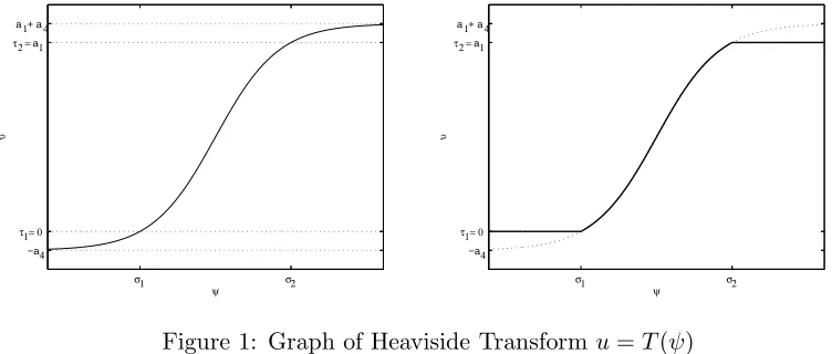
In order to impose a constraint on both the upper and lower bounds ofu, we have found that a suitable exponential type transform is the following

u= ˜Hǫ(ψ) =

w+ 2b

1 +e−ψǫ

−b

which resembles a smooth approximation to the Heaviside function given by

H(ψ) =

0, if ψ <0 1, if ψ_≥0,

whereǫ, b, w >0, and 0_{≈ −}b_≤H˜ǫ(ψ)≤w+b≈wdefines the intensity range forany ψ. Practically

one may take, for (3), b= 0.1, w = 255 to accommodate the commonly used rangeu_∈[0,255] and, for (27),b= 0.01, w= 1 to allow k_∈[0,1]. Note the inverse transformψ=₋ǫ₂logw_u+−_bu allows u= 0.

To allow generality, our proposed transform will be of the form

T(ψ) = a1+ 2a4 1 +a2e

−2ψ a3

where a= (a1, a2, a3, a4) and allaj’s are positive. Note 0≈ −a4 ≤u=T(ψ)≤a1+a4 ≈a1 for any ψ. As illustrated in Fig.1, the generality allows us to adjust the maximal and minimal values of the range using a1 and a4, the spread of usable range of ψ usinga3 and the point of u at which ψ will

be equal to zero usinga2. We can, if we wish, use this to restrict all values ofψ to positive but this is not necessary.

a + a

−a a

σ 1 σ 2

4 τ = 0₁ τ = _{2 1} 1 4

υ

ψ

a + a

−a a

σ 1 σ 2

4 τ = 0₁ τ = _{2 1} 1 4

υ

ψ

Figure 1: Graph of Heaviside Transform u=T(ψ)

Once the transform is specified, we now consider how to use it to reconstruct ψ first and hence the image u. The model (2) as studied in [34] can be transformed from

min

u f(u) =

1 2

Z

k(x₋x′, y₋y′)u(x′, y′)dΩ₋z(x, y)2

2+αL(u)

(with u_≥0) to the new problem forψ

min

ψ f(ψ) =

1 2

Z

k(x₋x′, y₋y′)T(ψ(x′, y′))dΩ₋z(x, y)2

2+αL(T(ψ)) (5)

whereL denotes the TV regulariser for (2) and theH1 for (9). The new and transformed model (5)

has no constraint on ψ and yet can ensure (3) to have a positive solution u. However, since both terms in (5) are non-linear in ψ, it remains to address the numerical solution methods.

In what follows, we shall propose to treat term 1 in (5) by linearisingT(ψ) (due to the challenge associated with a non-local operator k) and term 2 by lagged diffusion ideas (as for solving the denoising [34]).

Linearisation of T(ψ). The Taylor expansion of T(ψ) aboutψ= 0 is given by

T(ψ) =A+Bψ+O ψ2, A= a1+ 2a4 1 +a2 −

a4, B=

2a2(a1+ 2a4)

(1 +a2)2a3 .

Thus we can decomposeT(ψ) by separating its linear term in the form

u=T(ψ) =A+Bψ + ¯v¯( ˜ψ), v¯¯( ˜ψ) = ¯v( ˜ψ)₋A, v¯( ˜ψ) =T( ˜ψ)₋Bψ.˜

Iterative minimisation. Using the above decomposition, our solution strategy is as follows:

1: u(0) _←z andψ(0)_←T−1(u(0))

3: Solve forψ(ℓ+1)_{, givenψ}(ℓ)_{, from}

ψ(ℓ+1)_←min_kk_∗ψ(ℓ+1)B₋z¯(ψ(ℓ))_k2₂+α_kBψ(ℓ+1)) + ¯v(ψ(ℓ))_kβ_{T V} (_∗)

4: where ¯z(ψ(ℓ)_{) =z−k∗¯v(ψ}(ℓ)_).

5: end for

We now discuss how to solve the above equation (*) i.e.

min

ψ

f(ψ) = 1

2||Bk∗ψ−z¯||

2

L2_(Ω)+α

Z

Ω|∇

(Bψ+ ¯v)_|βdΩ

. (6)

Consider each term in turn. First letf1 = 1₂||Bk∗ψ−z¯||2_L2_(Ω) so minψf1 is given when∂f1/∂ψ = 0.

Here ∂f1 ∂ψ = ∂ ∂ψ 1

2||Bk∗ψ−z¯||

2

L2_(Ω) =

1 2

∂

∂ψ(Bk∗ψ−z¯) 2

=

∂

∂ψ(Bk∗ψ)

(Bk_∗ψ₋z¯) = (Bk)T(Bk_∗ψ₋z¯).

Second letf2=R_Ω∇(Bψ+ ¯v)dΩ and minψf2 is given when ∂

∂ǫ(f2(ψ+ǫφ))|ǫ→0 = 0 for an arbitrary

functionφ. We have

∂

∂ǫf2(ψ+ǫφ)

_ǫ →0 = ∂ ∂ǫ Z Ω|∇

(B(ψ+ǫφ) + ¯v)_|βdΩ

_ǫ →0 = Z Ω ∂

∂ǫ|∇(B(ψ+ǫφ) + ¯v)|βdΩ

_ǫ →0 = Z Ω

∇(B(ψ+ǫφ) + ¯v)

|∇(B(ψ+ǫφ) + ¯v)_|β · ∇BφdΩ

ǫ→0

=

Z

Ω

∇(Bψ+ ¯v)

|∇(Bψ+ ¯v)_|β · ∇BφdΩ

= ₋

Z

Ω∇ ·

∇(Bψ+ ¯v)

|∇(Bψ+ ¯v)_|β

!

BφdΩ +

Z

Γ

∇(Bψ+ ¯v)

|∇(Bψ+ ¯v)_|β ·Bφ~ndΓ.

We have therefore that minψ{f =f1+f2} is solved by

(Bk)T(Bk_∗ψ₋z¯) +α_{∇ ·} ∇(Bψ+ ¯v)

|∇(Bψ+ ¯v)_|β

!

B = 0 (7)

where ¯z= ¯z(ψ) =z₋k_∗¯v(ψ) and ¯v= ¯v(ψ) =T(ψ)₋Bψ.

Overall Algorithm. Assume u has a Dirichlet boundary condition. Then the discretised the Point Spread Function (PSF)kleads to a Block Toeplitz matrix with Toeplitz Blocks (BTTB) [22, 34]. In order to define the transform, we calculate the parameters a1, . . . , a4 according to the Appendix. We calculate the initial estimate ofψ(0) given the initial estimate ofu(0) as follows:

u=T(ψ) = a1+ 2a4 1 +a2e−

2ψ a3

−a4, ψ=T−1(u) =−

a3

2 ln

a1−u+a4 a2(u+a4)

.

Algorithm 1 A Transform based algorithm for positivity

1: function Trans_{(z, k, α, β,a, tol, maxit)}

2: u(0)_←z

3: Calculatea=_{a1, a2, a3, a4}

4: ψ(0)← −(a3/2) log a1+a4−u(0)/ a2(u(0)+a4)

5: forℓ_←1 tomaxitdo

6: Solve equation for ψ(ℓ+1) given ψ(ℓ), i.e.

ψ(ℓ+1) _← SOLVE (Bk)T _∗k_∗ψ(ℓ+1)₋z(ψ(ℓ))₋α_{∇ ·} ∇ Bψ

(ℓ+1)_−v(ℓ)

∇Bψb(ℓ+1)_−v(ℓ)

_β

= 0

7: wherez(ψ(ℓ)) =z−k∗v(ψ(ℓ)) and ψbdenotes a lagging fromψ. 8: end for

9: On exit,u(ℓ+1) _{←(a1+ 2a4)/(1 +a2exp(−2ψ/a3)).}

10: end function

4

Refinements and other solution strategies

4.1 Alternative Linearisation

In order to improve the speed of obtaining a solution, we carry out the Total Variation norm lineari-sation alongside the updating of the linearilineari-sation of the transform, thereby solving

(Bk)T _∗k∗ψ(ℓ+1)_−z¯(ψℓ_{)−α∇ ·} ∇ Bψ(

ℓ+1)_−v¯(ψℓ₎

_∇ Bψ(ℓ)_−v¯(ψℓ₎ β

= 0. (8)

In this way, we hope to get speed-up due to the saving of iterations on ψb. Experimental results are shown in Figure 8 and error values and CPU times for this method and the previous transform method are given in Table 6. It can be noted that, the reduction in CPU time is significant.

4.2 Alternative Regularisation

While the total variation semi-norm which we have used in our model gives good results for images which have sharp changes in intensity and hence jumps in the pixel intensity value, improved results may be found by considering alternative regularisation to treat smooth images. In this section, we consider a simple form of alternative regularisation using the L2 norm of the gradient of the image.

More robust regularizations are based on high order regularisers; see [10, 8, 28, 19].

In the traditional case, using a least squares fitting term andL2 as a regularisation term, we will

obtain a linear partial differential equation to solve. We give this minimizing functional as

f(u) = 1

2||k∗u−z||

2

L2

(Ω)+ α

2

Z

|∇u_|2dΩ. (9)

The well-known Euler-Lagrange equation for the imageu is therefore given by

Now referring to the above section, we substituteu=Bψ+ ¯vψ˜to (9)

f(u) = 1

2||k∗(Bψ+ ¯v

˜

ψ)₋z_||2_L2

(Ω)−α

Z

|∇(Bψ+ ¯vψ˜)_|2dΩ (11)

= 1

2||Bk∗ψ−z¯( ˜ψ)||

2

L2

(Ω)−α

Z

|∇(Bψ+ ¯vψ˜)_|2dΩ (12)

where ¯z(ψ) =z₋k_∗v¯ψ˜and ¯vψ˜=Tψ˜₋Bψ˜. The linearised Euler-Lagrange equation is

kT _∗Bk_∗ψ₋z¯ψ˜₋α∆Bψ+ ¯vψ˜= 0. (13)

4.3 Initialisation of u and k

Since there exist many efficient algorithms for solving models (2) and (3) without the positivity constraints, one idea of acquiring good initialisations foruandkis through applying such algorithms first.

In fact, the simplistic L2 method given by minimising (9) leads to solving the linear partial

differential equation (10) which can be done efficiently. We may therefore use the solution of it as the initial estimate u and then our transform model will offer a positive solution.

As we shall see from the next section, for model (3) with the unknown kernel k, the Vogel’s method [34] is no longer effective but we may use its result as an initial guess for our transform model; see Table 7 and Figure 9.

4.4 An Acceleration Algorithm for the Model

While our model performs well, it can often be rather slow to execute, particularly in cases of Gaussian blur. We address this issue using an alternating direction method (ADM) [15, 24, 36, 35]. We aim to separate our model into one of deblurring and one of denoising, each of which can be executed reasonable quickly. Starting with the unconstrained non-negative functional given by equation (5) we use the ADM to create the augmented Lagrangian functional

f(u, ψ, λ) = 1

2||k∗u−z||

2

L2

(Ω)+αL(Ta(ψ)) + γ

2||u−Ta(ψ)||

2

L2

(Ω)+< λ, u−Ta(ψ)> (14)

whereLrepresents either total variation (where we expect jumps in intensity) or L2 (where we expect smooth edges) i.e.

L(u) =

Z

Ω|∇

u_|βdΩ, or L(u) =

Z

Ω|∇

u_|2dΩ. (15)

Our aim is now to minimisef with respect tou,ψ and λ. Then we can give the Euler Lagrange equation for u:

kT _∗(k_∗u₋z) +γ(u₋Ta(ψ)) +λ= 0 (16)

and, rearranging, we have

where δ denotes the delta function and we can solve this using Fourier transforms. For additional support, we might add a term for u, given by χL1(u) where χ >0 and L1 is a regularisation term.

This model can be achieved by setting χ= 0.

For the second equation, we minimise with respect to ψ as follows. We must deal with the nonlinearity of the transform. We do this by considering the Taylor expansion given by

Ta(ψ) =A+Bψ+O(ψ2)

and approximate the transform with Ta(ψ) = Bψ+R(ψ) where R, the residual, is given by R =

Ta(ψ)₋Bψ. In practice, we will use this to form a fixed-point lagging technique by substituting

Ta(ψ,ψ˜) =Bψ+R( ˜ψ), lagging ˜ψ and updating until _||ψ₋ψ˜_||is sufficiently small.

−Bλ₋γBu₋(Bψ+ ˜R)+αL( ˜ψ)ψ= 0 (18)

where, for total variation,

L( ˜ψ)ψ= 4 ˜E1(a1+ 2a4)( ˜E1−1)|∇ψ|β (1 + ˜E1)3a23

− ∇ · 2(a1+ 2a4) ˜E1

(1 + ˜E1)2a3|∇ψ˜|β

∇ψ

!

.

Overall Algorithm

In order to solve our model, we begin with the initial estimate (typically the received image) and calculate the initial estimate of ψ using the chosen parameters. We then proceed to solve foru and

ψ, updating λ. Our algorithm is given below in Algorithm 2.

Algorithm 2 An Accelerated Transform based algorithm for positivity

1: function ATrans_{(z, k, α, β, γ, λ}(1)_{,a, tol, maxit)}

2: u(0)←z

3: Calculatea=_{a1, a2, a3, a4}

4: ψ(0)_{← −}(a3/2) log a1+a4−u(0)/ a2(u(0)+a4)

5: forℓ1←1 tomaxit do

6: forℓ2 ←1 tomaxitdo

7: Solve equation foru(ℓ2+1) _{given u}(ℓ2)_{, i.e.}

u(ℓ2+1)

← SOLVEkT(ku(ℓ2+1)

−z) +γ(u(ℓ2+1)

−(Bψ+ ˜R)) +χL1( ˜u(ℓ2))u(ℓ2+1)

=₋λ(ℓ1)

8: end for

9: forℓ3 ←1 tomaxitdo

10: Solve equation forψ(ℓ3+1) _{given ψ}(ℓ3)_{, i.e.}

ψ(ℓ3+1)

← SOLVE ₋γBu(ℓ2+1)

−(Bψ(ℓ3+1)

+ ˜R)+αL( ˜ψ(ℓ3))ψ(ℓ3+1)

=Bλ(ℓ1)

11: end for

12: Updateλ(ℓ1+1)

←λ(ℓ1)_{+γ u}(ℓ2+1)

−Ta ψ(

ℓ3+1)_.

13: end for

14: On exit,u(ℓ1+1)

←(a1+ 2a4)/(1 +a2exp(−2ψ(ℓ3+1)/a3)).

15: end function

4.5 A Reformulated Convex Model

new model is convex by the addition of a suitable term. We can then show convergence from the established approaches (see [23, 34, 5]). Tests in Section 5 will demonstrate that such a relaxation does not have a considerable impact on the solution or the quality of the restoration.

We aim to find an appropriate convex relaxation of this model by considering the fitting and regularisation terms separately since the sum of two convex functions is also convex. We attempt to obtain convexity of the fitting terms with the addition of a fitting term involving the function ψ of the form

µ

Z

Ω

(ψ₋ζ)2dΩ

where ζ is a function not depending on ψ and µ is a non-negative real constant which must be sufficiently large to make the model (14) convex. In fact we see that, for this model,µmay be quite small so that assuming close proximity of the arguments this term should have only a small impact on the results. ζ should be a function which is approximately equal to ψ but not depend on u so that convexity with respect to u is unaffected. We take ζ =T−1

a (z

∗_{) where}

z∗ = arg min

u

Z

Ω

(k_∗u₋z)2dΩ +α

Z

Ω|∇ u_|2dΩ

.

Actually any other similar model that can be solved efficiently will also suffice. The regularisation term requires a similar consideration for convexity, leading to

f(u, ψ;λ) = 1

2||k∗u−z||

2

L2

(Ω)+ γ

2||Ta(ψ)−u||

2

L2

(Ω)+< λ, Ta(ψ)−u >

+µ_||ψ₋ζ_||2_L2_(Ω)+α

Z

Ω

∇Ta(ψ) +θ_||ψ₋ζ_||2_L2_(Ω)

βdΩ. (19)

It turns out thatµ andθ must satisfy

µ_≥ 8 (a1+ 2a4)

27a2₃ (2γ(a4+Lu) +Lλ), θ≥ −

2(a1+ 2a4)(3√3−5)

3₋√33a2 3

. (20)

To give an example of the values for the parameters, if we assume that our image is contained in the range [0,1],_Lu=Lλ = 0, anda={1,1,0.44,0.01} foru=Ta(ψ), then µ≥0.04γ and θ≥ −1.

In order to minimise the functional, we first calculateζ and proceed with alternate minimisation. We present our overall algorithm below in Algorithm 3. For brevity, we do not present the Euler-Lagrange equation forψ but it can be calculated in a similar manner to those above.

We would now like to show that the functional defined above is convex.

Theorem 4.1 Let Ω _⊂ Rn be a non-empty convex subset of Rn and f : Ω _→ R∪ {+_∞} be the function defined by (19–20). Thenf is convex with respect to the argument ψ for ψ defined onΩ.

Proof. It is sufficient to show that the functional (19) is a sum of two convex functions. (i) The first part is given by

F(u, ψ) =

Z

Ω

γ(Ta(ψ)₋u)2+λ(Ta(ψ)₋u) +µ(ψ₋ζ)2dΩ. (21)

Algorithm 3 A deblurring algorithm based on convex formulation

1: function CTrans_{(k, z, λ}(1)_{;αs, γ, α, µ, θ)}

2: Solve the well known equation forζ from

z∗= min

u

n

fs(u) =||k∗u−z||_L22_(Ω)+α_s||∇u||2_L2_(Ω)

o

3: Calculatea={a1, a2, a3, a4}

4: u(0)_←z

5: ψ(0)_←T−1

a (z)

6: ζ_←Ta(P(z∗))

7: forℓ_←1 tomaxitdo

8: Solve equation for u(ℓ+1) givenu(ℓ), i.e.

u(ℓ+1)_← SOLVE (k†k+γδ)_∗u(ℓ+1) =k†z+λ(ℓ)+γTa

ψ(ℓ)

9: Solve equation for ψ(ℓ+1) _{given ψ}(ℓ)_{, i.e.}

ψℓ+1 _←min

ψ

n

fu(ℓ+1), ψ;λ(ℓ)o

10: Updateλℓ+1 =λℓ+γ u(ℓ+1)₋Ta ψ(

ℓ+1)

11: end for

12: On exit,u← Ta ψ(

ℓ+1)_.

13: end function

To show that (21) is convex, we require the second order derivative given by

∂2F(u, ψ)

∂ψ2 = 2µ−2J(ψ) [−2γ(Ta(ψ) +a4)a2E−(2γ(Ta(ψ)−u) +λ) (a2E−1)] (22)

to be non-negative, where J(ψ) = 2(Ta(ψ)+a4)a2E

(1+a2E)2a2₃ and E=E(ψ) := exp(−2ψ/a3).

It is not difficult to show that the term to the right ofJ(ψ) is contained in the bound (_−∞,2γ(a4+

Lu) +Lλ) whereLu andLλ are the lower bounds ofuand λrespectively. For the functionJ, we can

find that there is only one maximum by calculating the first derivative and finding the limits of the function as follows. We calculate the zero-point of the derivative

∂J ∂ψ =

12(a1+ 2a4)a22E2

(1 +a2E)4a33 −

4(a1+ 2a4)a2E

(1 +a2E)3a33

= 0 _⇔ ψ= a3

2 ln(2a2)

at which the functionJ is non-negative and strictly positive assuming that at least one ofa1 and a4

are non-zero, since a1, . . . , a4 are non-negative constants.

Taking limits now and noting that limψ→−∞E =∞and limψ→∞E= 0, we find that the function J tends to 0 at _±∞with a non-negative turning point given at ψ=a3ln(2a2)/2 which must be the

maximum.

lim

ψ→−∞

2a1+2a4

1+a2E

a2E

(1 +a2E)2a23

= lim

ψ→−∞

2 (a1+ 2a4)a2 1

E + 3a2+ 3a22E+a32E2

a2 3

= 0 (23)

lim

ψ→∞

2a1+2a4

1+a2E

a2E

Since the function tends to zero at both limits and has a single extremity, which is greater than or equal to zero, we can conclude that this is the maximum value and that the minimum is equal to zero, i.e.

J(ψ)_∈

0, Ja3

2 ln(2a2)

= 8 (a1+ 2a4) 27a2

3

.

Substituting these bounds and inequalities, including µ from (20), into (22), it is clear that the convexity condition ∂2F(u, ψ)/∂ψ2 _≥0 is satisfied.

(ii) For the (second part) total variation term, we begin by showing that if the function ω is convex then its total variation is also convex. It will then remain to show that the function (26) is convex given the restriction on the valueθ. Recall the definition of a total variation via duality [14]

G(ψ) =G(ω(ψ)) = sup

−

Z

Ω

ω(ψ)divφ dx:φ_∈C_c∞ Ω;RN,_|φ(x)_{| ≤}1_∀x_∈Ω

and, when ω = ω(ψ) is differentiable, ₋R_Ωω(ψ)divφ dx = R_Ωφ_{· ∇}ω(ψ)dx. Letting Lφ : ψ 7→ −RΩω(ψ)divφ dx, we would like to show that if ω is convex then G(ψ) is also convex. That is

∀ ψ1, ψ2 and t∈[0,1], we have G(tψ1+ (1−t)ψ2) ≤ tG(ψ1) + (1−t)G(ψ2).Assuming that ω(ψ)

is convex with respect to ψthen we have the relation

ω(tψ1+ (1−t)ψ2) ≤ tω(ψ1) + (1−t)ω(ψ2)

and

Lφ(tψ1+ (1−t)ψ2) ≤ tLφ(ψ1) + (1−t)Lφ(ψ2) ≤ tG(ψ1) + (1−t)G(ψ2) (25)

Since Gis the supremum of the functions Lφ, i.e.

sup

φ

Lφ(tψ1+ (1−t)ψ2) =G(tψ1+ (1−t)ψ2),

we have by (25) that G(tψ1+ (1−t)ψ2) ≤tG(ψ1) + (1−t)G(ψ2).That is, if the transformω(ψ) is

convex for ψ then the total variation is convex forψ. It remains to show that the function

ω(ψ) =Ta(ψ) +θ_||ψ₋ζ_||2_L2_(Ω), (26)

where ζ is as described above, is convex. Proceeding as in (i), we calculate the second derivative

∂2_ω

∂ψ2 = 2θ−2J1(ψ), J1(ψ) :=

2(a1+ 2a4)a2E(1−a2E)

(1 +a2E)3a23

.

We would like to find the upper bound of this function. We consider the limits

lim

ψ→−∞J1(ψ) = limψ→−∞

2(a1+ 2a4)a2E(1−a2E)

(1 +a2E)3_a2 3

= 0,

lim

ψ→∞J1(ψ) = limψ→∞

2(a1+ 2a4)a2E(1−a2E)

(1 +a2E)3a23

= 0,

which are equal to zero. We now find the extrema

∂J1

∂ψ = −8(a1+ 2a4)a2E

a2₂E2₋4a2E+ 1

a3₃(1 +a2E)4 = 0 ⇔ ψ =

−a3

2

2_±√3

at which J1 is given by

J1 −a3

2

2_±√3

a2

!

=₋2(a1+ 2a4)(2±

√

3) 1_±√3 3_±√33a2₃ .

It is easy to observe that a positive value is obtained at ψ=₋a3(2−√3)/2a2 and a negative value

is obtained atψ=₋a3(2 +√3)/2a2. We can therefore conclude that the values ofJ1 lie in the range

"

−2(a1+ 2a4)(3

√

3 + 5)

3 +√33a2 3

,2(a1+ 2a4)(3

√

3₋5)

3₋√33a2 3

#

,

so that ∂2ω(ψ)/∂ψ2 = 2θ₋2J1(ψ)≥0, ifθis from (20), as required.

5

Experimental results

Our experimental tests are hoped to show the effectiveness of image restoration by our Algorithm 1 in comparison with Vogel’s positivity method [4, 34], the projection method [15] and other methods that do not impose positivity constraints. We also compare with unconstrained (and partly constrained) models which have the constraint applied at the end by truncation or scaling. Specifically, in tables and figures, we denote the compared methods by these abbreviations:

• ROF: the well-known model (2) without positivity constraint.

• ROFT hr: the well-known model (2) with positivity and upper limit constraints applied at the

end by truncation.

• ROFSca: the well-known model (2) with positivity and upper limit constraints applied at the

end by scaling.

• Vogel: the non-negatively constrained restoration model by [4].

• VogelT hr: the non-negatively constrained restoration model by [4] with upper limit constraint

applied at the end by truncation.

• VogelSca: the non-negatively constrained restoration model by [4] with upper limit constraint

applied at the end by scaling.

• Proj: the constrained projection model by [15].

• New1: Algorithm 1 for model (5).

• New1L2: Algorithm 1 to solve the minimization of (9).

• New2: Algorithm 2 for model (14) i.e. an accelerated version of New1.

• MixL2TV: Algorithm 1 to solve (13) followed by Algorithm 1 to solve (7) using the solution of

(13) as the initial estimate.

• New3: Algorithm 3 for the reformulated model (19) i.e. the convex version of New2.

We use “Received” to mean the received imagez.

Seven sets of experimental results using 3 test images: the box-triangle image (Im1), the satellite image (Im2) and the retina image (Im3) are selected; see Figure 2. For the transform u=T(ψ), we choosea1 = 1,1.08,255 anda4= 10−2,10−2,0.5 respectively for the 3 test images (notea2, a3 are set

as in Appendix). For the blurring model (1), we have considered small and large levels of motion blur

(a) Im1 - Box-Triangle Image (b) Im2 - Satellite Image (c) Im3 - Retina Image

Figure 2: Test case images.

(Bl1 and Bl2 respectively) and small and large levels of Gaussian blur (Bl3 and Bl4 respectively); see Figure 3.

(a) Bl1 Shape (b) Bl1 Mesh (c) Bl1 Mesh

Close-up

(d) Bl2 Shape (e) Bl2 Mesh

(f) Bl3 Shape (g) Bl3 Mesh (h) Bl3 Mesh

Close-up

(i) Bl4 Shape (j) Bl4 Mesh

Figure 3: PSFs used for test cases. Images (a)-(c) show Bl1 - small motion blur, images (d)-(e) show Bl2 - large motion blur, images (f)-(h) show Bl3 - small Gaussian blur, and images (i)-(j) show Bl4 - large Gaussian blur.

There are several common measures for testing the quality of the restored image, including the following. We let utrue denote the true image, u the restored image, z the received image and letm

and nbe the number of pixels horizontally and vertically respectively. Then we have:

• Mean Squared Error (MSE) is given by M SE = _mn1 P_x,y(utrue(x, y)−u(x, y))2 and Root

Mean Squared Error (RMSE) is given by RM SE=√M SE.

• Signal-to-Noise Ratio (SNR) in dB is given by SN R= 10 log₁₀

P

x,y|utrue(x,y)| 2

P

x,y|utrue(x,y)−u(x,y)|2

• Peak Signal-to-Noise Ratio (PSNR) is given by P SN R= 20 log₁₀maxx,y|utrue(x,y)|

RM SE

Note that the RMSE is given by the L2 norm of the difference between the true image and the

restored image divided by the total number of pixels, i.e. RM SE = (1/mn)_||utrue−u||L2_(Ω). Given

astronomical images and images with significant amounts of black space, it is typically more common to use the L1 norm. We expect that these may provide more accurately descriptive measures of our data and the impact of the model in terms of non-negativity. We therefore propose the measures

• L1 Error given by

Er1 =||utrue−u||L1_(Ω)=

1

mn

X

x,y

|utrue(x, y)−u(x, y)|.

• A version of PSNR using theL1 norm of the difference between the true image and the restored

image is given by

Er2 = 20 log₁₀

_max

x,y|utrue(x, y)| Er1

.

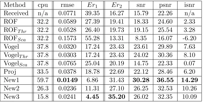
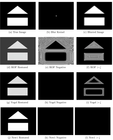
Model (1) with Gaussian blur. Result set 1 uses Im1 corrupted by Gaussian blur to demon-strate the effectiveness of the model in keeping the intensity values of the image constrained. We see in Figure 4 and Table 1 that [4] keeps the image positive but allows some points to take intensity values which are outside of the expected range, while [15] and the new models successfully keep the intensity values positive and within the expected range at all points.

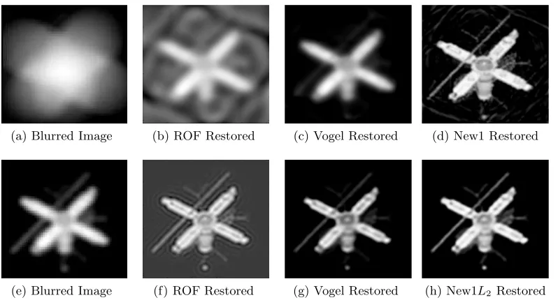
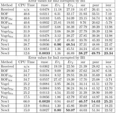
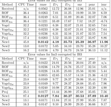
Model (1) with Motion blur. Result set 2 consists of Im2 and Im3 corrupted by small motion or small Gaussian blur. We see in Figure 5 and Tables 2–3 that for images corrupted by small levels of blur the results are competitive between the models. Error values are improved but visual quality is similar.

Model (1) with Heavy blurs. Result set 3 consists of Im2 corrupted by larger levels of blur (Bl2 and Bl4). We see in Figure 6 and Table 4 that that results are improved visually and in the error values for the new model in the case of Bl2. For Bl4, the Transform Model appears to be a closer approximation but the error values are similar.

Model (1) with Blur and a varying level of noise. Result set 4 consists of Im2 corrupted by Bl3 and varying amounts of noise (1% and 50%). We see in Figure 7 and Table 5 that visually the Transform model offers some improvement in quality while the error values are similar.

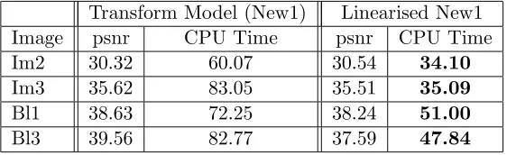
Model (1) by Algorithm 1 with alternative linerisation (8). Result set 5 shows in Figure 8 and Table 6 the results using the linearised Transform model. We can see that for the same quality of the restored image, the CPU time is improved.

Algorithm 1 combined with Vogel’s model. Result set 6 shows in Figure 9 and Table 7 examples using the received image as the initial estimate and the results of Vogel’s model as the initial estimate. We can see that this technique is useful for restoring the PSF given the image. In the case of the motion blur example, the CPU time is significantly improved and in the case of Gaussian blur, the error value is improved. In all cases, the visual quality is adequate.

Model (2) with Blurs. Now we consider the solution of model (3) for k. Result set 7 consists of motion and Gaussian blur PSFs which are regarded as being blurred by Im2. The task here is to recover the PSF given the true image. As the initial estimate, rather than taking the received data

Finally, to simultaneously restore bothu andkin the so-called blind deconvolution problem, the TV based model by [18] is the following

min

u

Z

Ω

(u_∗k₋z)2dΩ +α1_ku_kβ_{T V} +α2_kk_kβ_{T V}, s. t. k_≥0,

Z

Ω

k(s, t)dsdt= 1, (27)

whereα1, α2>0. Related studies can be found in [1, 11, 36, 32, 38]. In other experiments, we have

tried double transforms which appear to improve the robustness. This model will be investigated further in the future.

Method cpu rmse Er1 Er2 snr psnr isnr

Received n/a 0.0771 39.35 16.27 15.79 22.26 n/a

ROF 32.2 0.0589 27.39 19.41 18.33 24.60 2.33

ROFT hr 32.2 0.0528 26.40 19.73 19.15 25.54 3.28

ROFSca 32.2 0.1573 55.28 13.31 8.35 16.07 -6.20

Vogel 37.8 0.0320 17.24 23.43 23.61 29.89 7.63

VogelT hr 37.8 0.0303 17.24 23.43 24.02 30.36 8.10

VogelSca 37.8 0.0765 25.04 20.19 14.75 22.33 0.07

Proj 33.5 0.0378 18.78 22.69 22.12 28.46 6.20

New1 59.7 0.0149 6.86 31.43 30.28 36.55 14.29

New2 26.3 0.0236 11.31 27.10 26.25 32.53 10.26

New3 15.8 0.0241 4.45 35.20 26.02 32.35 10.09

Table 1: Result Set 1 - Error values for Im1 corrupted by Gaussian blur with no Noise. We can see that the error values are improved when using the Transform models and CPU time is improved by using New2–New3. As designed, the results of New2–New3 are very similar, showing that the additional term does not have a considerable effect on results.

6

Conclusion and Future Work

We have presented models to reconstruct images and PSFs and demonstrated that they can ensure positivity through introducing a transform and also keep the intensities of the restored data within the appropriate range. We have also demonstrated that the model offers competitive results in the case of small levels of blur and noise but much improved results in the case of corruption by larger levels of blur and noise. This model is particularly effective in giving a close approximation of the kernel (in the case where the image is known) which is of great importance in the case of blind deblurring. The transform idea is applicable potential to a class of other variational models. Since non-negativity is a significant criterion for blind deblurring models, we hope to consider such applications in the near future.

Appendix – Selection of Parameters in

T

(

ψ

)

The parametera1 is easily chosen, assuming knowledge of the bits-per-sample (bps) value of the true

image and the blurred image. This will typically be between 1 and 255 for images of bps 1 to 8 respectively, but can be quite low for the kernel. For example, a fairly compact-radius out-of-focus blur may have a kernel value upper limit of 10−2_{. While a larger value ofa}

1 should still give a good

approximation, it is essential that a1 be at least as large as the maximum image intensity value or kernel value and advisable that it be close to this. The parametera4 should be chosen in proportion

(a) True Image (b) Blur Kernel (c) Blurred Image

(d) ROF Restored (e) ROF Negative (f) ROF> ζ

(g) Vogel Restored (h) Vogel Negative (i) Vogel> ζ

(j) New1 Restored (k) New1 Negative (l) New1> ζ

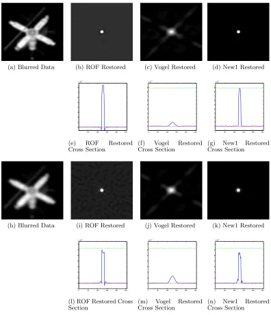
(a) Blurred Image (b) ROF Restored (c) Vogel Restored (d) New1 Restored

(e) Blurred Image (f) ROF Restored (g) Vogel Restored (h) New1 Restored

Figure 5: Result Set 2 - restoring images Im2 and Im3 corrupted by small motion blur Bl1 or small Gaussian blur Bl3. In some cases the results from the Transform model appear sharper than other models and more small detail is visible.

(a) Blurred Image (b) ROF Restored (c) Vogel Restored (d) New1 Restored

(e) Blurred Image (f) ROF Restored (g) Vogel Restored (h) New1L2 Restored

Error values for Im2 corrupted by Bl1

Method CPU Time rmse Er1 Er2 snr psnr isnr

Received n/a 0.0478 11.18 27.19 14.47 26.41 n/a

ROF 40.6 0.0211 6.31 32.17 21.93 33.51 7.10

ROFThr 40.6 0.0183 5.05 34.09 23.15 34.74 8.33

ROFSca 40.6 0.0932 25.81 19.93 9.76 20.62 -5.79

Vogel 31.9 0.0107 3.08 38.39 27.79 39.39 12.98

VogelThr 31.9 0.0107 3.08 38.39 27.79 39.39 12.98

VogelSca 31.9 0.0478 3.12 38.27 27.85 39.38 12.98

Proj 16.2 0.0054 1.37 45.40 33.76 45.33 18.92

New1 38.7 0.0036 0.96 48.54 37.31 48.88 22.47

New2 12.8 0.0051 1.36 45.51 34.24 45.81 19.40

New3 12.6 0.0033 1.16 46.89 38.27 49.75 23.34 Error values for Im3 corrupted by Bl1

Method CPU Time rmse Er1 Er2 snr psnr isnr

Received n/a 0.0362 19.19 22.50 21.39 28.82 n/a

ROF 34.7 0.0178 9.09 29.00 27.62 34.97 6.16

ROFThr 34.7 0.0164 8.52 29.55 28.33 35.69 6.88

ROFSca 34.7 0.0557 27.47 19.39 17.70 25.08 -3.74

Vogel 25.2 0.0084 3.95 36.24 34.14 41.51 12.70

VogelThr 25.2 0.0084 3.95 36.24 34.14 41.52 12.70

VogelSca 25.2 0.0113 4.54 35.02 31.39 38.90 10.09

Proj 17.5 0.0056 1.86 42.79 37.62 44.97 16.16

New1 66.0 0.0020 0.94 48.67 46.57 54.03 25.21

New2 12.9 0.0044 1.30 45.86 39.69 47.04 18.23

New3 15.0 0.0027 0.80 50.07 44.03 51.34 22.52

Error values for Im2 corrupted by Bl3

Method CPU Time rmse Er1 Er2 snr psnr isnr

Received n/a 0.0562 12.72 26.08 12.96 25.01 n/a

ROF 36.4 0.0263 7.01 31.25 19.99 31.59 6.59

ROFThr 36.4 0.0249 6.51 31.89 20.46 32.07 7.06

ROFSca 36.4 0.1221 33.49 17.67 7.52 18.27 -6.74

Vogel 32.2 0.0233 6.38 32.07 21.01 32.65 7.64

VogelThr 32.2 0.0233 6.38 32.07 21.01 32.65 7.64

VogelSca 32.2 0.0236 6.31 32.16 21.07 32.55 7.54

Proj 17.4 0.0203 5.52 33.33 22.27 33.87 8.86

New1 45.8 0.0142 4.18 35.73 25.39 36.97 11.96

New2 13.0 0.0172 5.05 34.10 23.70 35.28 10.27

New3 16.2 0.0156 4.70 34.73 24.58 36.13 11.12

Error values for Im3 corrupted by Bl3

Method CPU Time rmse Er1 Er2 snr psnr isnr

Received n/a 0.0422 24.01 20.56 20.04 27.49 n/a

ROF 35.2 0.0236 14.79 24.76 25.17 32.54 5.05

ROFThr 35.2 0.0226 14.35 25.03 25.56 32.93 5.44

ROFSca 35.2 0.0855 42.65 15.57 14.18 21.36 -6.12

Vogel 23.8 0.0169 9.77 28.37 28.06 35.44 7.95

VogelThr 23.8 0.0169 9.77 28.37 28.08 35.45 7.96

VogelSca 23.8 0.0240 10.98 27.36 24.68 32.39 4.90

Proj 25.1 0.0177 11.44 26.99 27.68 35.05 7.56

New1 87.4 0.0127 7.84 30.27 30.53 37.89 10.40

New2 13.1 0.0171 11.04 27.31 27.99 35.35 7.87

New3 16.3 0.0147 9.10 28.99 29.35 36.66 9.17

Error values for Im2 corrupted by Bl2

Method CPU Time rmse Er1 Er2 snr psnr isnr

Received n/a 0.22 63.17 12.80 -2.13 13.66 n/a

ROF 2.01 0.13 33.77 18.24 6.08 18.31 4.65

Vogel 16.02 0.11 26.55 20.33 7.30 19.71 6.05

New1 47.64 0.06 14.87 25.36 14.03 25.41 11.75

New1L2 30.18 0.07 18.68 23.38 11.77 23.33 9.67

MixL2TV 13.65 0.10 24.32 21.09 9.03 20.87 7.21

Error values for Im2 corrupted by Bl4

Method CPU Time rmse Er1 Er2 snr psnr isnr

Received n/a 0.0909 21.40 21.56 8.04 20.83 n/a

ROF 54.8 0.0596 14.98 24.66 12.72 24.49 3.66

Vogel 37.9 0.0565 13.00 25.88 13.11 24.96 4.13

New1 31.3 0.0489 11.72 26.78 14.45 26.22 5.39

Table 4: Result Set 3 - Error values for Im2 corrupted by Bl2 and Bl4. There is a noticeable improvement in the case of and while the results for Bl4 are competitive, the transform is slightly improved over competing models.

(a) Blurred Image (b) ROF Restored (c) Vogel Restored (d) New1 Restored

(e) Blurred Image (f) ROF Restored (g) Vogel Restored (h) New1 Restored

Figure 7: Result Set 4 - Restoring Im2 corrupted by Bl3 and 1% noise (top row) and 50% noise (bottom row). We can see that visually the Transform method appears to give improved results for weaker and stronger levels of noise.

(a) Im2 (b) Im3 (c) Bl1 (d) Bl3

Error values for Im2 corrupted by Bl3 and 1% noise.

Method CPU Time rmse Er1 Er2 snr psnr isnr

Received n/a 0.0479 11.34 27.07 14.49 26.40 n/a

ROF 42.1 0.0304 7.85 30.26 18.82 30.35 3.95

Vogel 12.1 0.0237 6.41 32.03 20.80 32.52 6.12

New2 4.9 0.0196 5.73 33.01 22.61 34.15 4.85 Error values for Im2 corrupted by Bl3 and 50% noise.

Method CPU Time rmse Er1 Er2 snr psnr isnr

Received n/a 0.0639 60.71 13.14 -13.24 12.59 n/a

ROF 15.00 0.0783 19.58 22.97 11.50 22.77 10.19

Vogel 5.64 0.0980 22.91 21.61 9.72 20.86 8.27

New1 55.76 0.0718 17.12 24.14 12.20 23.52 10.94

Table 5: Result Set 4 - Error values for Im2 corrupted by Bl2 and varying amounts of noise. We can see that the Transform model can offer improved results, particularly for larger levels of noise.

Transform Model (New1) Linearised New1

Image psnr CPU Time psnr CPU Time

Im2 30.32 60.07 30.54 34.10

Im3 35.62 83.05 35.51 35.09

Bl1 38.63 72.25 38.24 51.00

Bl3 39.56 82.77 37.59 47.84

Table 6: Result Set 5: Error values and CPU time for restoring images Im2 and Im3 as well as PSFs BL1 and BL3 using the Transform method and the Linearised Transform method. We can see that the quality of the restored image is not significantly different for each case but the CPU time is improved using the Linearised Transform method.

(a) Im2 (b) Im3 (c) Bl1 (d) Bl3

Figure 9: Result Set 6: Restored images and PSFs using the Linearised Transform method with the result of Vogel’s method as the initial estimate.

New1 MixVogTV

Image psnr CPU Time psnr CPU Time

Im2 30.54 34.10 30.61 39.79

Im3 35.51 35.09 35.71 46.83

Bl1 38.24 51.00 38.80 27.59

Bl3 37.59 47.84 42.53 51.14

(a) Blurred Data (b) ROF Restored (c) Vogel Restored (d) New1 Restored

50 100 150 200 250 0 1 2 3 4 5 6 7 8 x 10−3

(e) ROF Restored

Cross Section

0 50 100 150 200 250 −1 0 1 2 3 4 5 6 7 8 9 x 10−3

(f) Vogel Restored

Cross Section

0 50 100 150 200 250 −1 0 1 2 3 4 5 6 7 8 9 x 10−3

(g) New1 Restored

Cross Section

(h) Blurred Data (i) ROF Restored (j) Vogel Restored (k) New1 Restored

0 50 100 150 200 250 −1 0 1 2 3 4 5 6 7 x 10−3

(l) ROF Restored Cross Section

0 50 100 150 200 250 −1 0 1 2 3 4 5 6 7 x 10−3

(m) Vogel Restored

Cross Section

0 50 100 150 200 250 −1 0 1 2 3 4 5 6 7 x 10−3

(n) New1 Restored

Cross Section

We attempt to select the remaining parametersa2 and a3 in order to control the upper and lower

bounds of ψ as well as the value of ψ when u is equal to zero. In order to control the bounds, we define a length Σ =σ4−σ3 whereσ3 and σ4 represent two intensity values ofψ. We would then like

forτ4−τ3=T(σ4)−T(σ3) = Σ. From ψ(τ) =T−1(τ) =−a₂3ln

a1−τ+a4

a2(τ+a4)

, we have

Σ = σ4₋σ3 = ψ(τ4)₋ψ(τ3) (28)

= a3 2 ln

(a1₋τ3+a4)(τ4+a4) (τ3+a4)(a1−τ4+a4)

. (29)

So, assuming we fix Σ, τ3,τ4,a1 and a4, we have

a3=

2Σ

ln(a1−τ3+a4)(τ4+a4)

(τ3+a4)(a1−τ4+a4)

For our model, we fix the width Σ =τ4−τ3 (see Figure 11) and letτ4 =a1−τ3. Then, from 29,

we have

a3 = 2(τ4−τ3) ln(a1−τ3+a4)(τ4+a4)

(τ3+a4)(a1−τ4+a4)

= a1−2τ3 ln(a1−τ3+a4)

(τ3+a4)

.

The only remaining parameter whicha3 is dependent on and which has not already been decided is τ3. We find that τ3=a1/4 is adequate for the transform.

σ 3 σ 4 τ

3 τ 4

υ

ψ σ 3 σ 4

τ 3 τ 4

υ

ψ Σ

Σ

Figure 11: Graph of Heaviside Transformu=T(ψ)

We may use the parametera2 to control the value ofψ atu=T(ψ) = 0. We consider two cases: the first given by T(ψ) = a1/2 and the second given by T(ψ) = τ1 at ψ = 0 where τ1 is the lower

bound of ψ. The first option will make the graph pass through zero at the midpoint of the intensity values and the second will make all values of ψ naturally positive since the lower bound ofψ will be equal to zero. Letting u=T(ψ)

u= a1+ 2a4 1 +a2e

−2ψ a3

−a4.

Rearranging, we have

a2= a1+a4−u

e

−2ψ a3 (u+a

and so for the first case, we have

a2=

a1+a4−a1/2 a1/2 +a4 =

a1/2 +a4 a1/2 +a4 = 1,

and for the second case, we have

a2 = a1+a4−τ1

τ1+a4 .

In application, either of these will be sufficient to recover the image with similar results. In the case of the kernel, better results are obtained with a2 = 1. It is there advised therefore thata2 = 1

is the appropriate value for this parameter.

In summary, oncea1 anda4 are defined, the other quantities in the transformT(ψ) = a1+2a4 1+a2e

−2ψ a3

−

a4 can be determined automatically assuming that τ3 =a1/4 anda2 = 1 are acceptable.

References

[1] M. S. C. Almeida and L. B. Almeida. Blind and semi-blind deblurring of natural images. IEEE T. Image Process., 19(1):36–52, 2010.

[2] M. A. Bahnam and A. K. Katsaggelos. Digital image restoration. IEEE Signal Proc. Mag., 14(2):24–41, 1997.

[3] L. Bar, N. Sochen, and N. Kiryati. Semi-blind image restoration via Mumford-Shah regulariza-tion. IEEE T. Image Process., 15(2):483–493, 2006.

[4] J. M. Bardsley and C. R. Vogel. A nonnegatively constrained convex programming method for image reconstruction. SIAM J. Sci. Comput., 25(4):1326–1343, 2004.

[5] Aharon Ben-Tal and Arkadi Nemirovski. Lectures on modern convex optimization. SIAM pub-lications, 2001.

[6] F. Benvenuto, R. Zanella, L. Zanni, and M. Bertero. Nonnegative least-squares image deblurring: improved gradient projection approaches. Inverse Probl., 26(2):025004, 2009.

[7] Y Biraud. A new approach for increasing the resolving power by data processing. Astron. Astrophys., 1:124–127, 1969.

[8] K. Bredies, K. Kunisch, and T. Pock. Total generalized variation. SIAM J. Imaging Sci., 3:492–526, 2010.

[9] C. Brito-Loeza and K. Chen. Multigrid method for a modified curvature driven diffusion model for image inpainting. J. Comput. Math., 26(6):856–875, 2008.

[10] C. Brito-Loeza and K. Chen. Multigrid algorithm for high order denoising. SIAM J. Imaging Sci., 3(3):363–389, 2010.

[11] J. F. Cai, H. Ji, C. Liu, and Z. Shen. Framelet based blind motion deblurring from a single image. IEEE T. Image Process., 21:562–572, 2012.

[13] D. Calvetti, B. Lewis, L. Reichel, and F. Sgallari. Tikhonov regularization with nonnegativity constraint. Electron. Trans. Numer. Anal., 18:153–173, 2004.

[14] Antonin Chambolle, Vicent Caselles, Daniel Cremers, Matteo Novaga, and Thomas Pock. An introduction to total variation for image analysis.Theoretical foundations and numerical methods for sparse recovery, 9:263–340, 2010.

[15] R. H. Chan, M. Tao, and X. M. Yuan. Constrained total variational deblurring models and fast algorithms based on alternating direction method of multipliers. SIAM J. Imaging Sci., 6:680–697, 2013.

[16] T. F. Chan and K. Chen. On a nonlinear multigrid algorithm with primal relaxation for the image total variation minimisation. Numer. Algorithms, 41(4):387–411, 2005.

[17] T. F. Chan and L. A. Vese. Active contours without edges. CAM Report, UCLA, pages 98–53, 1998.

[18] T. F. Chan and C. K. Wong. Total variation blind deconvolution. IEEE T. Image Process., 7(3):370–375, March 1998.

[19] Q. Chang, X.-C. Tai, and L. Xing. A compound algorithm of denoising using second-order and fourth-order partial differential equations. Numer. Math. Theor. Meth. Appl., 2:353–376, 2009.

[20] K. Chen, E. Loli Piccolomini, and F. Zama. An automatic regularization parameter selection algorithm in the total variation model for image deblurring. Numer. Algorithms, pages 1–20, 2013.

[21] Y. Dong, M. Hinterm¨uller, and M. M. Rincon-Camacho. Automated regularization parameter selection in multi-scale total variation models for image restoration. J. Math. Imaging Vis., 40:83–104, 2011.

[22] C. Hansen, J. G. Nagy, and D. P. O’Leary. Deblurring Images: Matrices, Spectra, and Filtering. SIAM publications, 2006.

[23] Jean-Baptiste Hiriart-Urruty and Claude Lemar´echal. Convex Analysis and Minimization Al-gorithms: Part 1: Fundamentals, volume 305 ofA Series of Comprehensive Studies in Mathe-matics. Springer, 1993.

[24] Y. Huang, M. K. Ng, and Y.-W. Wen. A fast total variation minimization method for image restoration. Multiscale Model. Simul., 7:774–795, 2008.

[25] D. Kundur and D. Hatzinakos. Blind image deconvolution.IEEE Signal Proc. Mag., 13(3):43–64, May 1996.

[26] D. Kundur and D. Hatzinakos. Blind image deconvolution revisited. IEEE Signal Proc. Mag., 13(6):61–63, Nov 1996.

[27] R. L. Lagendijk, I. Biemond, and D. E. Boekee. Regularized iterative image restoration with ringing reduction. IEEE T. Acoust. Speech, 36(12):1874–1888, 1988.

[29] L. Rudin, S. Osher, and E. Fatemi. Nonlinear total variation based noise removal algorithms.

Physica D, 60:259–268, 1992.

[30] M. I. Sezan and A. M. Tekalp. Survey of recent developments in digital image restoration. Opt. Eng., 29(5):393–404, May 1990.

[31] M. I. Sezan and H. J. Trussell. Prototype image constraints for set-theoretic image restoration.

IEEE T. Signal Proces., 39(10):2275–2285, 1991.

[32] Q. Shan, J. Jia, and A. Agarwala. High-quality motion deblurring from a single image. InACM SIGGRAPH 2008 Papers, 2008.

[33] Y. Shi, Q. Chang, and J. Xu. Convergence of fixed point iteration for deblurring and denoising problem. Appl. Math. Comput., 189:1178–1185, 2007.

[34] C. R. Vogel. Computational Methods for Inverse Problems. SIAM, 2002.

[35] F. Wang. Alternating Direction Methods for Image Recovery. PhD thesis, Hong Kong Baptist University, 2012.

[36] W. Wang and M. K. Ng. On algorithms for automatic deblurring from a single image. J. Comput. Math., 30:80–100, 2012.

[37] Y. Wen and R. H. Chan. Parameter selection for total variation based image restoration using discrepancy principle. IEEE T. Image Process., 21:1770–1781, 2012.