Toward Realizable Quantum Computers

Thesis by

Michael Edward Beverland

In Partial Fulfillment of the Requirements for the degree of

Doctor of Philosophy

CALIFORNIA INSTITUTE OF TECHNOLOGY Pasadena, California

2016

© 2016

Michael Edward Beverland ORCID: [Author ORCID]

ACKNOWLEDGEMENTS

I have been very lucky to have been surrounded by many inspiring scientists while a graduate student at Caltech.

Firstly, I would like to thank my advisor, John Preskill, for always finding time to hear me out when I wanted to explain my often underdeveloped ideas. He will always be my role model as a physicist. Along with John, I would also like to thank the rest of my thesis committee: Xie Chen, Alexei Kitaev, and Gil Refael.

I have also received valuable mentorship from my main collaborators Alexey Gor-shkov, Gorjan Alagic, Fernando Pastawski, and Krysta Svore. Their guidance has been invaluable.

Special thanks goes to my officemate, collaborator and good friend Aleksander Kubica. I have had many other exceptional collaborators deserve a lot of credit for the work presented in this thesis: Gretchen Campbell, Jeongwan Haah, Ana Maria Rey, Michael Martin, Andrew Koller, Hector Bombin, Robert Koenig, Sumit Sijher, and Oliver Buerschaper.

John’s group meetings have been a hub for quantum information and have provided much inspiration. Regular attendees during my time include, Ning Bao, Mario Berta, Thom Bohdanowicz, Peter Brooks, Todd Brun, Darrick Chang, Elizabeth Crosson, Nicolas Delfosse, Andrew Essin, Glen Evenbly, Bill Fefferman, Matthew Fishman, Steve Flammia, Alexey Gorshkov, David Gosset, Nick Hunter-Jones, Joe Iverson, Stacey Jeffery, Stephen Jordan, Isaac Kim, Olivier Landon-Cardinal, Netanel Lindner, Shaun Maguire, Prabha Mandayam, Spiros Michalakis, Roger Mong, Evgeny Mozgunov, Leonid Pryadko, Kirill Shtengel, Sujeet Shukla, Kristan Temme, and Beni Yoshida.

ABSTRACT

The work in this thesis splits naturally into two parts: (1) experimentally oriented work consisting of experimental proposals for systems that could be used to imple-ment quantum information tasks with current technology, and (2) theoretical work focusing on universal fault-tolerant quantum computers which we hope can be scaled as experimental capabilities continue to move forward. Chapters one, three, and four are based on published work Michael E. Beverland et al.,2016; Koller et al., 2014; Michael E Beverland et al.,2016; Kubica and M. Beverland,2015. Chapters two and three cover currently unpublished work (at the time of writing).

In the first chapter we propose trapping cold atoms in a square-well to robustly implement a spin hamiltonian which is naturally protected from the dominant source of noise. The key feature is that the system’s Hamiltonian has parameters which are independent of the spatial degrees of atomic motion which is not the case for spin hamiltonians made with other traps or a different type of atom. The Hamiltonian is highly symmetric (invariant under both on-site spin rotations and site permutations), and exactly solvable. This highly symmetric spin model should be experimentally realizable even when the vibrational levels are occupied according to a high-temperature thermal or an arbitrary non-thermal distribution.

After analyzed the experimental aspects of the proposal and a few direct applications in the first chapter, in chapter two we focus on a particular application for which the system is particularly well suited: spectrum estimation of unknown density matrices. The symmetry group of the Hamiltonian is precisely the group which is relevant for the Young diagram algorithm to measure density matrices Keyl and Werner,2001. The highly entangled Young diagram measurements are performed naturally via standard Ramsey spectroscopy in our system, when prepared with a copy of the unknown density matrix in the nuclear spin of each atom.

for storing quantum information and can result in high error thresholds. In chapter three, we consider the fault-tolerant processing of information in such codes. As opposed to studying braiding of anyons, about which much was already known, we considered the action of locally generated unitary logical gates. Locally generated logical gates of topological codes are intrinsically fault tolerant because spatially localized errors remain localized, and therefore correctible. They are also expected to be much easier to implement than braiding in some settings. Unfortunately, we find severe limitations on the locally generated logical gates. No code in this class has a universal set of locally generated gates, and topological codes which support anyons which are universal for braiding have no non-trivial locally generated gates. Abelian models have locally generated gates restricted to the Clifford group. We derive these results by relating logical gates of a topological code to automorphisms of the Verlinde algebra of the corresponding anyon model.

Although are results are negative, there are ways around them. Firstly, braiding is known to be universal for some topological codes, although they may be hard to implement in practice. There is a standard approach Sergey Bravyi and Alexei Kitaev, 2005, using resource states, to complete the universal gate set for a code which admits the full (but non-universal) Clifford group. These resource states cannot be fault-tolerantly generated in the code, but they can be distilled so that many noisy resource states can be traded for fewer resource states with less noise. The drawback is that this approach involves very significant overhead, which accounts for the vast majority of the quibits required in the realistic overhead estimates Austin G Fowler et al.,2012.

Although in chapter three we find that two-dimensional topological codes have severe restrictions on the locally generated gates that can occur, in higher dimensional topological codes there is considerably more freedom. In chapter four we describe a three-dimensional topological code for which one can use locally generated unitaries (along with local measurement) to achieve a universal gate set. Our work is based on ideas from Bombín’s paperGauge Color Codes[arXiv:1311.0879v3]. We show how to transversally implement the generalized phase gate Rn = diag(1, e2πi/2n) in an

PUBLISHED CONTENT AND CONTRIBUTIONS

Beverland, Michael E et al. (2016). “Protected gates for topological quantum field theories”. In:Journal of Mathematical Physics57.2, p. 022201.

Beverland, Michael E. et al. (2016). “Realizing exactly solvable SU(N) magnets with thermal atoms”. In:Phys. Rev. A93 (5), p. 051601.

Koller, A. P. et al. (2014). “Beyond the Spin Model Approximation for Ramsey Spectroscopy”. In:Phys. Rev. Lett.112, p. 123001.

Kubica, Aleksander and Michael Beverland (2015). “Universal transversal gates with color codes: A simplified approach”. In:Physical Review A91.3, p. 032330.

TABLE OF CONTENTS

Acknowledgements . . . iii

Abstract . . . iv

Published Content and Contributions . . . vii

Table of Contents . . . viii

I Small quantum computers

1

1.1 Background and Motivation . . . 2

1.2 Spin Hamiltonian: ground electronic level only . . . 5

1.3 Exact eigenenergies and eigenstates . . . 6

1.4 Robustness to imperfections . . . 10

1.5 Experimental proposal: spin diffusion dynamics . . . 12

1.6 Derivation of spin-diffusion dynamics . . . 13

1.7 Spin Hamiltonian: ground and first excited electronic levels . . . 17

1.8 Experimental proposal: GHZ state preparation . . . 18

1.9 Derivations for GHZ state preparation . . . 21

1.10 Experimental Details . . . 22

1.11 Outlook . . . 26

Chapter II: Spectrum Estimation . . . 27

2.1 Motivation and Background . . . 27

2.2 Overview of the proposal . . . 29

2.3 Spectrum estimation forN = 2 . . . 31

2.4 Generalization to arbitraryN . . . 33

2.5 Expectation value of the number operator . . . 34

2.6 Variance of the number operator (ongoing work) . . . 38

2.7 Experimental Considerations . . . 40

2.8 Outlook . . . 41

II Scalable quantum computers

42

3.1 Introduction . . . 43

3.2 TQFTs: background . . . 51

3.3 Constraints on locality-preserving automorphisms . . . 66

3.4 Global constraints from the mapping class group . . . 71

3.5 Global constraints fromF-moves on then-punctured sphere . . . 79

3.6 The Fibonacci and Ising models . . . 86

3.8 Density on a subspace and protected gates . . . 100

3.9 Simplifications from excited states . . . 102

Chapter IV: Code switching. . . 106

4.1 Introduction . . . 106

4.2 Color code in two dimensions . . . 108

4.3 Color code in higher dimensions. . . 115

4.4 Transversal gates in color codes . . . 121

4.5 Universal transversal gates with color codes . . . 126

4.6 Acknowledgements. . . 131

Chapter V: Overhead of code switching and state distillation . . . 132

5.1 Quantum computing overhead . . . 133

5.2 Delfosse decoder . . . 137

5.3 Two-dimensional color code thresholds . . . 144

5.4 Code switching – dimension jump . . . 149

5.5 Overhead for code switching . . . 152

5.6 Magic state distillation . . . 155

5.7 Overhead for state distillation . . . 158

5.8 Outlook . . . 160

Part I

Small quantum computers

C h a p t e r 1

A NATURALLY PROTECTED SYMMETRIC HAMILTONIAN

In this chapter we propose the use ofn thermal fermionic alkaline-earth atoms in a flat-bottom trap to robustly implement a spin model which is naturally protected from noise. The key feature is that the system’s Hamiltonian has parameters which are independent of the spatial degrees of atomic motion which is not the case for spin hamiltonians made with other traps or a different type of atom. The hamiltonian displays two symmetries: theSnsymmetry that permutes atoms occupying different vibrational levels of the trap and the SU(N) symmetry associated with N nuclear spin states. The high symmetry makes the model exactly solvable, which, in turn, enables the analytic study of dynamical processes such as spin diffusion in this SU(N) system. We also show how to use this system to generate entangled states that allow for Heisenberg-limited metrology.

This highly symmetric spin model should be experimentally realizable even when the vibrational levels are occupied according to a high-temperature thermal or an arbitrary non-thermal distribution.

1.1 Background and Motivation

(unless the traps are operated near surfaces, which can reduce spacings and increase energy scales Gullans et al.,2012; Romero-Isart et al.,2013; González-Tudela et al., 2015), it is a significant challenge in experimental cold atom physics to achieve temperatures and decoherence rates low enough to access superexchange-based quantum magnetism.

Since ultracold atoms can be prepared in specific internal (i.e. spin) states with extremely high precision, spin temperatures that can be realized are much lower than the experimentally achievable motional temperatures. It is therefore tempting to circumvent the problem of high motional temperature by constructing a spin model in such a way that the motional and spin degrees of freedom are effectively decoupled. We provide a recipe for such a decoupling and hence for realizing spin models with thermal atoms.

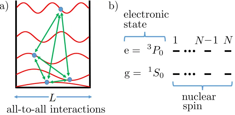
The first crucial ingredient for implementing such a spin model is to depart from second-order superexchange interactions and use contact interactions to first order Gibble,2009; A. M. Rey, A. V. Gorshkov, and Rubbo,2009; Yu and Pethick,2010; Pechkis et al., 2013; C. Deutsch et al., 2010; Maineult et al.,2012; Hazlett et al., 2013; Martin et al., 2013; Swallows et al., 2011; Koller et al., 2014. As shown in Fig. 1.1(a), this can be achieved if all atoms sit in different orbitals of the same anharmonic trap and remain in these orbitals throughout the evolution, which is a good approximation for weak interactions Martin et al.,2013; Swallows et al.,2011;

a)

b)

electronic

state

e =

P

g =

S

1

N

1

N

nuclear

spin

all-to-all interactions

Gibble,2009; A. M. Rey, A. V. Gorshkov, and Rubbo,2009; Yu and Pethick,2010. In that case, the occupied orbitals play the role of the sites of the spin Hamiltonian. However, because of high motional temperature in such systems, every run of the experiment typically yields a different set of populated orbitals and hence a different spin Hamiltonian Martin et al.,2013. Thus, unless the dynamics are constrained to states symmetric under arbitrary exchanges of spins Martin et al., 2013, every run of the experiment would lead to different spin dynamics.

The second crucial ingredient of our proposal to decouple spin and motion is therefore to use an infinite one-dimensional square-well potential as the anharmonic trap, with the motion frozen along the other two directions. The interaction terms in the spin Hamiltonian H are proportional to the squared overlap of pairs of distinct sinusoidal orbitals, and are thus all of equal strength. ThereforeHˆ is independent of which orbitals are occupied, leading to spin-motion decoupling and temperature independent predictions, as well as opening up the possibility of precise control. Moreover, sinceHˆ is invariant under any relabeling of the noccupied orbitals, Hˆ hasSnpermutation symmetry.

Alkaline-earth atoms enrich the symmetry. In such atoms, the vanishing electronic angular momentumJ in the electronic clock statesg =1S0 ande =3P0 results in the decoupling of the nuclear spin I fromJ [Fig.1.1(b)]. This endowsHˆ with an additional SU(N) spin-rotation symmetry, whereN can be tuned between 2 and

2I+ 1by choosing the initial state A. V. Gorshkov, Hermele, et al.,2010; M. A. Cazalilla, Ho, and Ueda, 2009; X. Zhang et al., 2014; Scazza et al., 2014; Guido Pagano et al., 2014; Cappellini et al., 2014. Restricted to g, Hˆ is just the sum of spin-swaps over all pairs of occupied orbitals and can be diagonalized in terms of irreducible representations of the group of symmetriesG=Sn×SU(N).

Motional-temperature-insensitive spin models can also be realized using long-range interactions between ions in Paul traps Sorensen and Klaus Molmer,1999, Penning traps Richerme et al., 2014; Jurcevic et al., 2014; Britton et al., 2012, and also between molecules Micheli, Brennen, and Zoller,2006; Barnett et al.,2006; A. V. Gorshkov, Manmana, et al.,2011; Yan et al.,2013or Rydberg atoms Schauß et al., 2012 pinned at different sites of an optical lattice. However, the realization of

SU(N)-symmetric spin models in such systems requires a great deal of fine tuning Alexey V. Gorshkov, Hazzard, and Ana Maria Rey,2013.

Gogolin, 2015, especially in the presence of long-range interactions Richerme et al., 2014; Jurcevic et al.,2014, we first study spin diffusion Sommer et al., 2011; Koschorreck et al., 2013; Yan et al., 2013 in a system of g atoms only. Due to crucial use of representation-theoretic techniques, our calculations are not only ex-ponentially faster than naive exact diagonalization but also, for N = 2, yield a closed-form expression for all n. We then present a protocol that employs both

g and e states to create Greenberger-Horne-Zeilinger (GHZ) states Greenberger, Horne, and Zeilinger,1989, which could be used to approach the Heisenberg limit for metrology and clock precision Bollinger et al.,1996.

1.2 Spin Hamiltonian: ground electronic level only

A single mass-M fermionic alkaline-earth atom (for now, in its ground electronic stateg) trapped in a 1D spin-independent potentialV(x)has real orbitalsφj(x)with energiesEj satisfying[−(~2/2M)∂2/∂x2+V(x)]φj(x) =Ejφj(x). The operator

ˆ

c†_jpcreates an atom from the vacuum inφj(x)with nuclear spin statep∈1,2, ..., N. For n identical atoms in the same potential with contact s-wave interactions, the Hamiltonian isHˆ =P_jpEjˆcjp† ˆcjp+P_p<qP_jkj0_k0Ujkj0k0ˆc†_jpcˆj0pˆc†kqcˆk0q, where

Ujkj0k0 = 4π_~ω_⊥agg

Z ∞

−∞

dxφj(x)φk(x)φj0(x)φk0(x), (1.1)

andagg is the 3D-scattering length, and a potential with frequencyω⊥ freezes out transverse motion.

To obtain the desired highly symmetric Hamiltonian, we specialize to the case whereV(x)is a width-Linfinite square well, with well-known eigenstatesφj(x) =

p

2/Lsin(jπx/L) for0 ≤ x ≤ L, with energyEj = (πj/L)2/2M. Then Ujkj0k0

is zero unless (i): (j ± k) = ±(j0 ± k0); to first order in the interaction, we can also set Ujkj0k0 → 0 unless P_jpEjˆc†jpcˆjp is conserved, which occurs when (ii): j2 +k2 = j02 +k02. Conditions (i) and (ii) are both satisfied if and only if

(j0, k0) = (j, k)or(k0, j0) = (j, k). As the system conserves orbital occupancies, it can be described by a spin model. Assuming orbitals are at most singly occupied (nˆj =Ppˆcjp† cˆjp ≤1for allj)1, the spin Hamiltonian is:

ˆ

H =₋UX

j<k

ˆ

sjk, (1.2)

1

where ˆsjk ≡ Ppqˆc†jpcˆjqcˆ†kqˆckp swaps spins j andk, and the sum is over occupied orbitals. Crucially, U ≡ 4πagg~ω⊥/L is independent ofj andk. We dropped a constantPjEj +n(n−1)U/2, which will have no effect on spin dynamics. For a fixed set of occupied orbitals,Hˆ hasNnbasis states|p1, p2, ..pniwithpj ∈1, ..., N.

1.3 Exact eigenenergies and eigenstates

ForN = 2, the spin-swap can be written in terms of the Pauli operators: ˆsjk = 1/2+

(ˆσx jσˆkx+ˆσ

y jσˆ

y

k+ˆσjzσˆkz)/2, allowing Eq. (1.2) to be written asHˆ =−U

h

~ S2₊ n

4(n−4)

i

, whereS~ = 1₂Pj~σj. The eigenstates ofHˆ forN = 2are therefore the well-known Dicke Dicke,1954states|S, Sz, ki, with energies

E(S) = ₋UhS(S+ 1) + n

4(n−4) i

.

The quantum numberklabels distinct states with the sameS~2 andSˆz eigenvalues. We now describe the general case for arbitraryN.

The Hamiltonian in equation (1.2) has two obvious symmetries: permutations inSn of then occupied orbitals, and application of the same unitary inSU(N)to all of the spins. Define a unitaryUˆ( ˆV , σ)which permutes occupied orbitals by σ ∈ Sn and implements the spin rotationVˆ ∈SU(N):

ˆ

U( ˆV , σ)_|p_1i|p2i...|pni ≡ Vˆ|pσ−1(1)iVˆ|p_σ−1(2)i...Vˆ|p_σ−1(n)i. _(1.3)

These unitaries (for all Vˆ ∈ SU(N) and σ ∈ Sn) form a well-understood repre-sentation of the groupG = Sn×SU(N). Each unitaryUˆ( ˆV , σ) commutes with

ˆ

H = −UP

j6=kˆsjk. Irreps of SU(N)and Sn are both uniquely labeled by Young diagrams. AYoung diagramis a pictorial representation of~λconsisting of a row of

λ1 boxes above a row ofλ2 boxes, which is above a row ofλ3 boxes etc. It is also useful to define~γ= (γ1, γ2, ..., γλ1)as the column heights of the Young diagram~λ.

a) b) c)

3 1 0 0 6 1 0 1

2 3

4 5

6 7 |1i |2_i

|3i

|1i |1_{i |}1_i

|2i

6U

2U

0U

2U

d)

S

SU

(N

)

de

ge

ne

rac

y

/N

n

e)

-450 -400 -350 -300 -250 -200 -150 -100

10-9

10-6

10-3

Energy

E

(

~

)

/U

Figure 1.2: (a) An example Young diagram ~λ = (4,2,1) [with ~γ = (3,2,1,1)] for n = 7, N = 3. (b) A labeling of boxes in ~λ from 1 to n, increasing down columns, starting at the left. (c) Orbitals associated with boxes in thepth row of the Young diagram are put in spin state|pito form basis state|Ti =|1231211i[spins ordered as in (b)], used to construct eigenstate |~λi = |A{123}i|A{12}i|11i with

E(~λ)/(₋U) = P

i λi

2

−P

j γj

2

= 6 + 1 + 0₋3₋1₋0₋0 = 3. (d) The set of all Young diagrams forn = 4andN = 3, with energies above. Below each diagram, every eigenstate is represented by a colored box: starting with any given eigenstate, rotations inSU(N)generate linear combinations of eigenstates in the same column, while permutations in Sn generate linear combinations of eigenstates in the same row. Representative states are found using the prescribed construction to be|1111i,

(_|12_{i − |}21_i)_|11_i,(_|12_{i − |}21_i)(_|12_{i − |}21_i), and(|123i+|312i+|231i − |132i − |213_{i − |}321_i)_|1_i, respectively. (e) Spectrum for n = 30with N = 2 (red), and

A Young diagram~µlabels an Irrep ofSU(N)if and only if it has at mostN rows:

~µ= (µ1, µ2, ..µN). On the other hand, a Young diagram~ν, labels an Irrep ofSnif and only if its elements sum ton: Piνi =n.

Each irrep of the product groupG=Sn×SU(N)is the tensor product of an irrep ofSU(N)and an irrep of Sn and is therefore uniquely labeled by a pair(~µ, ~ν). A consequence of Schur-Weyl duality is that representation (1.3) block-diagonalizes into exactly one copy of each irrep ofGsatisfying~µ=~ν, and no other irreps Bacon, I. L. Chuang, and Harrow,2007; Fulton and Harris,1991. Therefore for each Young diagram~λ = (λ1, λ2, .., λN)such that Piλi = n, there is a subspace of constant energyE(~λ). One can form an unnormalized projection operatorΠˆ_L(~λ) into the~λ subspace Fulton and Harris,1991:

ˆ

Π_L(~λ) = X

c∈col(T)

r∈row(T)

sgn(c) ˆU( ˆI, c) ˆU( ˆI, r). (1.4)

Here, L(~λ)is the labeling of boxes in the Young diagram~λfrom1 ton as shown in Fig.2.3(b), and row(L)(col(L)) is the group of all permutations of the numbers

1 to n that preserve the contents of rows (columns) of L(~λ). Applying ΠˆL(~λ) to any state that it does not annihilate returns an eigenstate of energy E(~λ). For concreteness we use|Ti ≡ |1,2, ..., γ1i |1,2, ..., γ2i...|1,2, ..., γλ1i, where we also

define~γ = (γ1, γ2, ..., γλ1)as the column heights of the Young diagram~λ. For each ~λwe obtain an explicit eigenstate: |~λi= ˆΠL(~λ)|Ti. Now we describe how to obtain the eigenvalueE(~λ)such that:

ˆ

H|~λi=E(~λ)|~λi. (1.5)

Premultiplying byhT|we obtain: E(~λ) =hT|Hˆ|~λi =−UPj6=khT|ˆsjk|~λi, noting thathT|~λi = 1. For j, k in the same column of the labeled Young diagramL(~λ), we know thatsˆjk|~λi = −|~λi. Similarly forj, k in the same row of L(~λ)we have hT_|ˆsjk =hT|. Thus pairs(j, k)in columns contribute−1toE(~λ)and pairs(j, k) in rows contribute+1. The number of such pairs can be counted, hence:

E(~λ)/(−U) =

N

X

i=1

λi

2

− λ1

X

j=1

γj

2

+ X

{j6=k}diagonal

hT|sˆjk|~λi, (1.6)

suffices to consider the case j > k). Therefore, hT|sˆjk|~λi = hT|sˆkmsˆjm|~λi = −hT_|ˆskmsˆjm|~λi = 0, implyingE(~λ)/(−U) =PNi=1

λi

2

−Pλ1

j=1 γj

2

. Therefore the energy of the Hamiltonian is simply the number of ways of choosing two boxes in the same row of ~λ, minus the number of ways of choosing two boxes in the same column. This is in line with the intuition that the swap picks up−U for each symmetric pair and+Ufor each antisymmetric pair in the Young diagram. In terms of~λ,

E(~λ) = ₋U 2

N

X

i=1

(λi−2i+ 1)λi. (1.7)

Figure 2.3(d) illustrates the eigenvalues and eigenstates of Hˆ for the simple case of n = 4 and N = 3, along with the corresponding Young diagrams. There is an equivalence for the SU(2) case between Young diagram (λ1, λ2) and angular momentum quantum numberSgiven byS = (λ1−λ2)/2 = (2λ1−n)/2.

Now we show how to create an eigenstate in any~λ-subspace. First consider the basis state: |Ti ≡ |1,2, ..., γ1i |1,2, ..., γ2i... |1,2, ..., γλ1i, which is chosen by

associating orbitals with boxes of the Young diagram as in Fig.2.3(b), and putting those orbitals in spin states as in Fig. 2.3(c). We form|~λi(which is one of many eigenstates in the~λ-subspace) by antisymmetrizing|Tiover orbitals associated with boxes in each column of~λ:

|~λi=_|A{12...γ_1}i|A{12...γ_2}i..._|A{12...γλ1}i, (1.8)

where A{...} antisymmetrizes its argument, for example: |A{123}i = |123i+ |312_i +_|231_{i − |}132_{i − |}321_{i − |}213_{i. The normalization constant is fixed by}

h~λ|~λi=γ1!γ2!...γλ1!.

To understand and label the other eigenstates in the~λ-subspace, we note that there are three (equivalent) views of how the fullNn dimensional Hilbert space H de-composes. Firstly, H decomposes into a single copy of each~λ-irrep of the group

Sn×SU(N)for each valid Young diagram~λ. Secondly,Hdecomposes intok~λSnk

copies of each~λ-irrep of SU(N)for each valid Young diagram~λ. Thirdly, H de-composes intok~λSU(N)kcopies of each~λ-irrep ofSnfor each valid Young diagram

~λ. Here, k~λSnk and k~λSU(N)k are the dimensions of ~λ irreps of Sn and SU(N),

respectively.

|~λ,1,1_i = _|~λ_i in the ~λ-subspace, one can obtain the set of orthonormal states {|~λ,1, b_i}forb= 1,2, ...,k~λSnkfrom linear combinations ofUˆ( ˆI, σ)|~λ,1,1iforσ ∈ Sn. Similarly, from each state |~λ,1, bi, one can form the set of orthonormal states {|~λ, a, bi}for a = 1,2, ...,k~λSU(N)k from linear combinations ofUˆ( ˆV , I)|~λ,1, bi forVˆ ∈SU(N). ForN = 2, this picture is the familiarDicke ladder, in which states are grouped into blocks of equalS, withSzincreasing downwards andkincreasing to the right.

The dimensions of each block can be calculated using the standard hook-length formulae Sagan, 2000 for any given Young diagram~λ. In particular, the ground-state spaces for U > 0 (ferromagnetic interaction) andU < 0 (antiferromagnetic interaction) are ~λF = (n,0,0, ...,0) and ~λAF = (n/N, n/N, ..., n/N) and have dimensionsDF andDAF, respectively:

DF =

(n+N −1)!

n! (N ₋1)! , DAF =

n! [(n/N)!]N

N−1

Y

i=1

i!

[n/N +i]. (1.9)

1.4 Robustness to imperfections

In this Section, we consider deviation from a perfect infinite square-well potential

V(x). For simplicity, we consider the case in which all atoms are in the ground elec-tronic state. The interaction Hamiltonian Eq. (1.2) becomes: Hˆ0 =−P_j<kUjkˆsjk, whereUjk = (U L/2)

R

φ2

j(x)φ2k(x)dx, andφj(x)is a single-particle orbital, which is a sine function in the ideal case. AsHˆ0 is a weighted sum of termssˆjk and there-fore hasSU(N)symmetry, it cannot mix states in different~λ-subspaces. However asHˆ0 does not exhibitSnsymmetry, the~λsubspace does not have a single energy -but breaks intoD(~λ)energy subspaces,D(~λ)is the dimension of the~λirrep ofSn. We write the eigenenergies ofHˆ0 asE0(~λ, b), withblabeling distinct energies. Provided that the inhomogeneity inUjkis small, i.e. that|Ujk−U| U, the energy splittingsE0(~λ, b)within each~λsubspace will be small compared to energy separa-tions between different~λsubspaces. Exact determination ofE(~λ, b)can be carried out by projectingHˆ0onto the~λsubspace and solving the resulting matrix equation, which is computationally difficult as the matrices have dimensionO(exp(n)). Here we are satisfied with an indication of the magnitude of deviation from the ideal energy eigenvalues. We seek the offset: ∆E(~λ)≡ _D(~λ)1 PD(~λ)b=1

h

E0₍~λ, b_)−E(~λ₎i

and the variance: σ2(~λ)≡ _D(~λ)1 PD(~λ)b=1

h

−U n(n₋1)/2, where~λ0 = (n,0,0, ..,0), one can show that

∆E(~λ) = − E(~λ)

E(~λ0)

! X

j<k

(Ujk −U). (1.10)

Note that

E(~λ) E(~λ0)

≤1for all~λ. The main technical lemma used to prove this is that

for any operatorOˆ, D(~λ)

X

b=1

h~λ, b|Oˆ|~λ, bi= D(~λ)

n! X

σ∈Sn

h~λ, b0_|σ−1_{Oσˆ |~λ, b}0_i,

(1.11)

where the latter sum is over all permutationsσin the symmetric groupSn. Modeling

Ujk as a set of n(n−1)/2 independent random variables with mean U, one can similarly show that

σ2(~λ) = 

1− E(~λ)

E(~λ0)

!2

 X

j<k

h(Ujk−U)2i, (1.12)

where hi indicates that we have taken the ensemble average over realizations

footnote2 of ∆Ujk, which simply allows us to set h∆Ujk∆Uj0k0i = 0 _where

j, k ₆=j0_{, k}0

. These results indicate that the deviations in energy levels from those for the exact case caused by inhomogeneity inUjk generically behave as∼ n∆U. This is because, to estimate∆E(~λ), we assume thatP_j<k(Ujk−U)is the sum of

n(n−1)/2uncorrelated positive and negative terms each of magnitude∼∆U, and similarly for the varianceσ2(~λ), except all terms are positive. We therefore expect that, in order to seeprevivals of the kind shown in Fig.1.3of the main text, we need to pick up small phase errorsn∆U t. 1over timet ∼p/U, which corresponds to

∆U/U .1/(np).

However, note that most symmetric ~λ subspaces (which have E(~λ)/E(~λ0) close to unity), experience less splitting due to inhomogeneity in Ujk, although they do experience an overall shift. For the GHZ protocol, the~λ subspaces involved are

(n,0), (n −1,1) and (n −2,2), which will shift relative to one another under inhomogeneity inUjk by an amount independent ofnfor largen.

functionsφj(x)are

φj(x) =

r 2

Lsin (jπx/L) +

8

π2

αL2/ ~

2_π2

2M L2

X

k k6=j

jk(₋1)j+k

(j2_−k2₎3

r 2

Lsin (kπx/L).

Substitution intoUjk =U L

R

φ2

j(x)φ2k(x)dxyields exact expressions for the first or-der corrections toU, which (for alljandk) satisfy: |Ujk−U|<10−2

αL2_/ ~2π2

2M L2

U+

O(α2₎

. The inhomogeneity is therefore strictly less than one percent if the mag-nitude of the perturbation is approximately of the same order as the characteristic energy of the square well. The size of the deviations fall off at the fourth power of

j, k, such that for ensembles of atoms,∆U is typically much better than this bound suggests.

1.5 Experimental proposal: spin diffusion dynamics

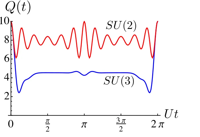
Spin diffusion is the process by which evolution under a generic spin Hamiltonian causes initially ordered states to diffuse Sommer et al., 2011; Koschorreck et al., 2013; Yan et al., 2013. We take initial state |ψ(0)i = |1i⊗m1|2i⊗m2...|Ni⊗mN. Note that any computational basis state can be changed to this form by reordering occupied orbitals. We consider the time evolution of observableQˆ =Pm_j=11 |1ijh1|j: the number of the firstm1 orbitals in spin-state|1i. This is the simplest observable capturing the broken symmetry of the initial state. The expectation of Qˆ evolves according to: Q(t)≡ hψ(0)|eiHtˆ Qeˆ −iHtˆ |ψ(0)i, omitting~where convenient from here on.

Calculation of such a time evolution for a generic Hamiltonian requires matrix diag-onalization, which scales exponentially withn(for fixedN). Using the symmetry of Hamiltonian (1.2) and the Wigner-Eckart theorem forSU(N), we obtain an explicit sum (see section1.6) forQ(t) in terms of Clebsch-Gordan and recoupling coeffi-cients. For the case ofN = 2, with initial state ofm1 =mspin up andm2 =n−m spin down orbitals, using well-known closed forms for the Clebsch-Gordan and recoupling coefficients:

Q(t) = m+

n/2

X

S=|n−2m|/2+1

γ(S)[cos (2SU t)₋1], (1.13)

whereγ(S) = 4S

2_−(n−2m)2

4S

n n/2+S

/ _n−n_m

evolution of the same operator and total particle number for initial states withN = 2 spin states andN = 3spin states. The oscillations are much less pronounced and spin diffusion occurs more fully (Qdrops lower) for the latter state. With this model, looking at times away from the multiples of the revival time2π/U, one could study apparent near-equilibration of some observables (such as Q in the N = 3 case) acting on the firstm1 spins. Perturbations could be added to the system to remove revivals and potentially allow for the thermalization of the firstm1 spins.

U t

0

p

₂

p

3

₂

p

2

p

2

4

6

8

10

_SU

₍₂₎

SU

(3)

Q

(

t

)

Figure 1.3: Exact time evolution underHˆ of an operatorQˆ =Pj=110 |1ijh1|j, which counts the number of the first ten orbitals in spin state |1i. Two initial states are compared: |1i⊗10|2i⊗20forSU(2)and|1i⊗10|2i⊗10|3i⊗10forSU(3). Although the evolution is the same for short times, theSU(3) case results in significantly more diffusion of spin state|1iout of the first four orbitals at later times. Since allE(~λ) are integer multiples of U, complete revival occurs at U t = 2π. In the SU(2) case, the oscillation is dominated by the smallestS in Eq. (1.13). This is consistent with the fact that for fixedSz, the size of the eigenspaces decreases withS, causing overlap to be larger with subspaces of smallS generically.

1.6 Derivation of spin-diffusion dynamics

In this Section, we present the derivation of the spin-diffusion dynamics, first for

N = 2and then for generalN.

We are concerned with observable Qˆ = Pmj=11 |1ijh1|j. In this section, we use the notation that for any operatorAˆ, A(t) ≡ hψ(0)|eiHtˆ Aeˆ −iHtˆ |ψ(0)i, where|ψ(0)i= |1i⊗m1|₂i⊗m2_...|_Ni⊗mN

systems, we outline the N = 2 case first before covering the general case more abstractly.

For N = 2, we can choose the angular momentum (Dicke) basis to span the Hilbert space: |S, Sz, ki, which diagonalizes the Hamiltonian: Hˆ|S, Sz, ki = −U S(S + 1)|S, Sz, ki(dropping a constant energy). The initial state is |ψ(0)i = |↑i⊗m|↓i⊗n−m where we used|↑iand|↓iin place of|1iand|2i. This state can be understood as a tensor product of two Dicke states on subsets of spins: |ψ(0)i = |m/2, m/2_i⊗|(n₋m)/2,₋(n₋m)/2_{i, where there is no need for a}kquantum num-ber since states with|Sz|=Shave no additional degeneracy. The tensor product of two angular momentum states can be written as a sum of “total” angular momentum states: |ψ(0)i=P_SC(S)|S, Sz=m−n/2, α(S)i, whereC(S)is a Clebsch-Gordan coefficient, andα(S)represents the fact that|S, Sz=m−n/2, α(S)iis some specific linear combination of Dicke states with the sameSandSz, but differentk’s. Hence,

Q(t) = P

S,S0C(S0)∗C(S)eiU t[S(S+1)−S 0_(S0_+1)]

hS0, Sz, α(S0)|Qˆ|S, Sz, α(S)i. Note thatQˆ =mIˆ+ ˆSmz withS~m =Pmj=1S~j, andSˆmz is the0-component of the(S = 1) -spherical tensor Tˆ ≡ {Sˆm−1,Sˆmz,Sˆm+1}, with Sˆm±1 = ∓( ˆSmx ±iSˆmy)/

√

2. We first apply the Wigner-Eckart theorem to write the matrix element in terms of the re-duced matrix element and a Clebsch-Gordan coefficient. Then, sinceTˆ ≡ Tˆm⊗Iˆ acts only on the firstmspins, we rewrite Rose,1957; J. Brown and Carrington,2003 the reduced matrix element on the full system in terms of one on the first mspins and a recoupling coefficient:

hS0, S_z0, α(S0)_|Qˆ_|S, Sz, α(S)i=mδS,S0 _(1.14)

+hm/2||TˆL||m/2i

(

1 m/2 m/2

(n₋m)/2 S0 _S

)

(h1,0| ⊗ hS, Sz|) |S0, Szi0 ,

where(h1,0| ⊗ hS, Sz|) |S0, Sz0iis a Clebsch-Gordan coefficient andhm/2||TˆL||m/2i is the reduced matrix element ofTˆLon theS =m/2state of the firstmspins. The recoupling coefficient

(

SA SB SAB

SC S SBC

)

≡ hS, Sz,(SAB, SC)|S, Sz,(SA, SBC)i

is the overlap between two states of givenSandSz formed from the tensor product of three subsystems withSA, SB and SC in two different ways: by combining A andB to formSAB first, and by combiningBandCto formSBC first. Substitution of the Clebsch-Gordan and recoupling coefficients into the matrix element gives Eq. (1.13).

⌦ ⌦ ⌦

m1 m2 mN

=

⌦

~_A ~_B ~_C

~_AB

~_BC ~

~

0 adj

I

In m1

a) b)

c)

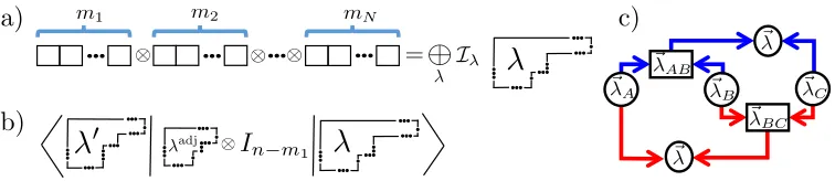
Figure 1.4: (a) Initial state |ψ(0)i can be written in terms of energy eigenstates: |ψ(0)i =|11...1i|22...2i...|N N...Ni=P

λ,a,αC(λ, a, α)|λ, a, αi. (b) Key simpli-fications arise in the matrix elementhλ0, a0, α|Q|λ, a, αi(which is used to calculate

Q(t)) since: Qˆ is a component of a “spherical tensor” forSU(N)(allowing us to make use of the Wigner-Eckart theorem) and has support only on the firstm1 sites. (c) The recoupling coefficient is defined by taking the direct product of three irreps

A, B andC, and finding the overlap between two copies of the same irrep found in two ways: by combiningA and B first (top), and by combining B and C first (bottom).

as a direct product of spin-symmetric states |ψ(0)i = ⊗mj=1|1 1i ⊗mj=12 |2i...⊗mj=1N |N_i = _|κ1, a1i|κ2, a2i...|κN, aNi, where ai labels the particular state in the κi ≡

(mi,0, ...0) irrep which corresponds to |ii⊗mi. The product of κ = (m,0, ...,0) with any irrep λ0 has no multiplicity Bacon, I. L. Chuang, and Harrow, 2007: |κ, ai|λ0, a0i=P

λ00_,a00C(λ00, a00)|λ00, a00i, where each irrepλ00appears at most once

andC(λ00, a00)≡ hλ00, a00|(|κ, ai|κ0, a0i)is a Clebsch-Gordan coefficient. Applying this iteratively, starting from the right, |ψ(0)i = Pλ,a,αC(λ, a, α)|λ, a, αi, where

α labels the set of intermediate irreps, C(λ, a, α) can be expressed in terms of Clebsch-Gordan coefficients, and|λ, a, αiare orthogonal eigenstates: H|λ, a, αi=

E(λ)_|λ, a, α_{i. Note:} a _∈ 1,2, ...,dim[λSU(N)] labels a basis state within the λ -irrep of SU(N), and eachα labels one distinct copy (out of dim[λSn] copies) of

the λ-irrep of SU(N) in the Hilbert space H = (CN)⊗n (all copies of irrep λ of SU(N) in H sit inside a single copy of irrep λ of Sn×SU(N)). Therefore:

Q(t) = P

λ,λ0_,a,a0_,αC∗(λ0, a0, α)C(λ, a, α)ei[E(λ

0_)−E(λ)]t

hλ0_{, a}0_{, α|Q|λ, a, αi, where} we setα0 =αsinceQhas support only on the firstm1spins. We now outline tools to determine the matrix elementhλ0, a0, α|Q|λ, a, αi.

The states|λ, a, αitransform according to matrix irrepDλofSU(N):V⊗n|λ, a, αi=

P

a0Daλ0_a(V)|λ, a0, αi. For each N, there is a set of single-spin operators which generateSU(N): τadj ≡ {t1, t2, ..., tN2−1}_{which transform according to}Dadj_(the

adjoint irrep λ_adj): V⊗ntaV†⊗n = P_a0Dadj_a0_a(V)ta0. The set {t1, t2, ..., tN2₋₁,Iˆ}

hλ0_{, a}0_{, α|Q|λ, a, αi = c}

0+Pa00ca00hλ0, a0, α|T_aadj₀₀|λ, a, αi, whereT_aadj = Pm_j=11 t_{a j}

andQ=Pmj=11 |1ijh1|j ≡

Pm1

j=1qˆj. We now prove a generalization of Eq. (1.14) to determine the matrix elementhλ0, a0, α0|Taadj00|λ, a, αi[see Fig.1.4(b)]. We will need the Wigner-Eckart theorem and recoupling coefficients forSU(N):

hλ0, a0, α0_|T_aλ0000|λ, a, αi =

X

I

(_hλ0, a0,_I||λ00, a00_i|λ, a_i) _hλ0, α0_||Tλ00_||λ, α_iI,(1.15)

(

λA λB λAB

λC λ λBC

)

IAB,IC;IBC,IA

≡ hλ, a,(λAB,IAB,IC)|λ, a,(λBC,IBC,IA)i. (1.16)

Note that multiplicityIappears in the Wigner Eckart theorem forN >2[Eq. (1.15)], since the tensor product of irreps can include multiple appearances of the same irrep. The recoupling coefficient defined in Eq. (1.16) relates two copies of the same irrep

λ formed from the tensor product of three irreps: λA, λB, and λC, but combined in different orders [see Fig. 1.4(c)]. To define notation: λA andλB are combined to make λAB, whose different copies are labeled byIAB, whileIC labels different copies ofλwhenλAB is combined withλC.

One can decompose|λ, a, αi=Pa1,a2C

λ,a

κ1,a1;λ2,a2|κ1, a1i|λ2, a2i, whereλ2is

spec-ified byα, and

Cκλ,a1,a1;λ2,a2 ≡(hκ1, a1|hλ2, a2|)|λ, a, αi (1.17)

Substituting intohλ0, a0, α|Taadj00|λ, a, αiand applying Eq. (1.15) to the firstm1spins: hλ0, a0, α|Tadj

a00|λ, a, αi=hκ1||Tadj||κ1i

X

a1,a01,a2

¯

Cκλ10,a,a00₁;λ2,a2C

λ,a

κ1,a1;λ2,a2C

κ1,a1

κ1,a0₁;λadj_,a00

=hκ1||Tadj||κ1i

X

I1

(

λadj _κ

1 κ1

λ2 λ0 λ

)∗

I1

Cλ0,a0,I1

λadj_,a00_;λ,a. (1.18)

The second line represents the generalization of Eq. (1.14). To derive Eq. (1.18), we return to the abstract scenario of three irreps λA, λB and λC used to define recoupling coefficients in Eq. (1.16). First write|λ, a,(λAB)ias a linear combination of|λ, a,(λBC,IA)iwith Eq. (1.16) as coefficients in the special case whereλB =

λAB = κ (allowing us to dropIAB, IC andIBC). Rewriting states on both sides as the direct product of states in each of the three subsystems, multiplying by CλC,aC

λ0

BC,aBC;λB,aB, summing overλ

0

BC, and using orthogonality gives:

X

aAB,aB,aC

Cλλ,aAB,aAB;λC,aCC

λAB,a1AB

λA,aA;λB,aBC

λC,aC

λBC,aBC;λB,aB =

X

IA

(

λA κ κ

λC λ λBC

)∗

IA

Using Eq. (1.18), the time evolutionTa(t)≡ hψ(0)|exp (iHt)Taexp (−iHt)|ψ(0)i, and thereforeQ(t), is written as an efficiently computable sum (containingpoly(n) terms Alex et al.,2011, each calculated inpoly(n)operations):

Ta(t) = hκ1||Tadj||κ1i

X

λ01,a01,λ1,a1;α

C∗(λ0₁, a0₁, α)C(λ1, a1, α)e(i[E(λ

0

1)−E(λ1)]t)

(1.20)

×X I1

(

λadj _κ

1 κ1

λ2 λ01 λ1

)

I1

[_hλ0₁, a0₁,_I1|(|λadj, ji|λ1, a1i)].

The group-theoretic method presented in this Section was crucial for obtaining the analytical result for SU(2) [Eq. (1.13)]. It is also crucial for doing numerics for

SU(N >2)for largen. However, for sufficiently small n, such as the one shown in Fig. 3, one can do the SU(N > 2)numerics using the following simpler method. One first constructs a complete basis of fully symmetric states for the firstm1spins, for the nextm2 spins, for the nextm3 spins, etc... Then one combines them into a basis for the full system and keeps only those states that havem1 1’s,m2 2’s, m3

3’s, etc... It is straightforward to evaluate the Hamiltonian in this reduced basis and then numerically exponentiate it to calculate time evolution.

1.7 Spin Hamiltonian: ground and first excited electronic levels

In this section, we derive the Hamiltonian describing identical (bosonic or fermionic) multi-component particles in an infinite square well interacting vias-wave interac-tions. We then specialize to the case of fermionic alkaline-earth atoms. This section generalizes the hamiltonian derived in Section 1.2 to the case of multiple energy levels, which will be needed in the following section on the proposal for producing GHZ states.

Contact interactions between two identical multi-component fermionic (bosonic) atoms are described by the Hamiltonian

ˆ

H_int12 = 4π~ω⊥δ(x1−x2)⊗A,ˆ (1.21)

where the operator Aˆonly has a physical effect on exchange antisymmetric (sym-metric) two-particle internal states because exchange symmetric (antisym(sym-metric) spatial states do not interact. In second quantized form, where cˆ†jr creates an atom in internal state r and orbital φj(x) with non-interacting energy Ej, and

Wk0_j0_jk = (4π_~ω_⊥)R₀Ldx φ_k0(x)φ_j0(x)φ_j(x)φ_k(x)_{. The interaction becomes:}

ˆ

infinite square well of widthL, to first order in the interaction, only terms satisfying

(j0_{, k}0_{) = (j, k)}

or (j0, k0) = (k, j) survive. Additionally assuming no multiple occupancies, we obtain Wkjjk = Wjkjk = W ≡ (4π~ω⊥)/L for j 6= k, and the Hamiltonian becomes:

ˆ

H = X

j,r

Ejcˆ†jrˆcjr (1.22)

+WX

j,k

X

r0,s0,r,s

hs0, r0|Aˆ|r, si ˆc†_jr0cˆ†ks0cˆjrˆcks+ ˆc†kr0cˆ†js0ˆcjrˆcks

.

Now we specialize to the case focused on in our work. For fermionic alkaline-earth atoms,Aˆcannot depend on nuclear spin; therefore (denoting the identity on nuclear spin byIˆN),

ˆ

A= aee|e, eihe, e|+agg|g, gihg, g|+a+eg|e, gi+he, g|++a−eg|e, gi−he, g|−

⊗IˆN,

where |e, gi± = (|e, gi ± |g, ei)/√2 A. V. Gorshkov, Hermele, et al., 2010. Under these conditions, and applying a strong magnetic field (which to first order in perturbation theory prevents exchanges |ep, gqi ↔ |eq, gpi for p 6= q), we obtain Eq. (5) withU1g2g = U2g1g = Ugg ≡ 4πω⊥agg/L, U1e2e = U2e1e = Uee ≡

4πω_⊥aee/L, U1g1e =U2g2e = 4πω⊥a−eg/M, U1g2e =U2g1e = 2πω⊥(a+eg+a−eg)/M. Recently discovered orbital Feshbach resonances may be used to further tune the values ofU1g2eandU2g1eR. Zhang et al.,2015; G. Pagano et al.,2015; Höfer et al., 2015.

1.8 Experimental proposal: GHZ state preparation

To create a GHZ state, we allow atoms in the excited electronic stateewith an energy

ωeg above the ground electronic stateg [see Fig.1.1(b)]. First assumeN = 2. An applied magnetic field adds Zeeman spin-splittings Bg 6= Be Boyd, Zelevinsky, Ludlow, Foreman, et al.,2006to bothgandestates. To first order in the interaction strength, the spin Hamiltonian is (see section1.9for details) :

ˆ

H = Hˆsp+

X

α<β

Uαβ ˆnαnˆβ −

X

j6=k

ˆ

c†_jαˆcjβˆc†kβˆckα

!

. (1.23)

The single-particle Hamiltonian isHˆsp =ωegnˆe+Bg(ˆn1g−nˆ2g) +Be(ˆn1e−nˆ2e), the sum α < β is over distinct pairs of 1g, 1e, 2g and 2e, and the constantsUαβ are derived in terms of (electronic-state dependent) scattering lengths. Note that

ˆ

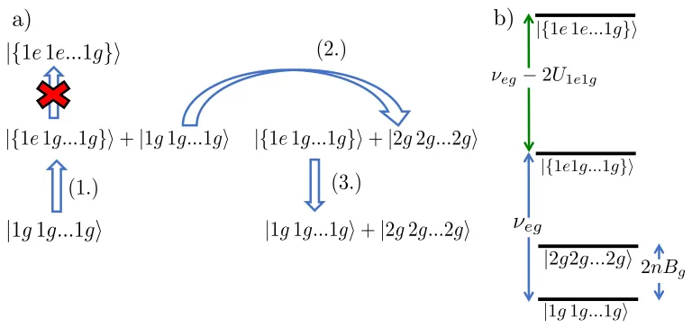
n1g,nˆ2g,nˆ1e andnˆ2eare separately conserved by Hamiltonian (1.23). As shown in Fig.1.5, to create then-particle GHZ state(|1g1g..1gi+|2g2g..2gi)from|1g1g..1gi, three consecutive pulses should be applied:

1. Spatially inhomogeneous, weak, many-bodyπ/2pulse

e−iνegt X

j

Ωeg_j (|1eijh1g|j +|2eijh2g|j) +h.c.

with frequencyνeg =ωeg+ (Be−Bg) +nU1e1g.

2. Spatially uniform, weak, single-atom π pulse e−iν12tΩ12P_j(|2gijh1g|j + |2eijh1e|j) +h.c.with frequencyν12 = 2Bg.

3. Pulse 1, but for pulse areaπ, notπ/2.

The frequency of the first pulse picks out an effective two-level system consisting of |1g1g..1gi and |{1e1g..1g}i ∝ Pjp(Ω

eg

j − Ω¯eg)|1eijh1g|j|1g1g..1gi (we de-finedΩ¯eg ≡P_jΩegj /n.). The pulse must be spatially inhomogeneous to makeΩ

eg j

|{1e1e...1g_}i

|1g1g...1g_i

(1.)

(2.)

(3.)

|{1e1g...1g_}i+_|1g1g...1g_{i |{}1e1g...1g_}i+_|2g2g...2g_i

|1g1g...1g_i+_|2g2g...2g_i

a)

b)

|{1e1e...1g_}i

|1g1g...1g_i

|{1e1g...1g_}i

⌫eg

|2g2g...2gi ⌫eg 2U1e1g

2nBg

Figure 1.5: (a) System is prepared in|1g1g..1gi, and spatially inhomogeneous pulse (1.) results in an equal superposition of this state and|{1e1g..1g}i, which has onee atom. An interaction blockade prevents coupling to states with twoeatoms. Pulse (2.) flips the spins of the all-g state. The initial pulse is reversed in pulse (3.), resulting in the GHZ state. (b) Relevant energy levels of the Hamiltonian with e andg states and the magnetic field. Note that pulses (1.) and (3.), which involve states|1g1g..1giand|{1e1g..1g}i, do not couple to state|{1e1e..1g}isince there is a blockade of2U1e1g. Similarly, during pulse (2.), blockade prevents the excitation of state|{1e1g..1g}i.

|2g2g..2g_i state because the pulse is off-resonant by energy of order (Be −Bg). Note that although the precise form of the inhomogeneity in the first pulse is unim-portant, the final pulse and the first pulse must have the same inhomogeneity. Since all three pulses rely on blockade, each pulse must take time 1/U. Curiously, the fact that the interactions in our spin model have effectively infinite range makes our spins analogous to long-range interacting Rydberg atoms, for which a similar protocol exists for generating maximally entangled states Saffman and K. Molmer, 2009. Note that we have designed the protocol to have at most onee atom at any time, which avoids the potential problem of inelastice-ecollisions Traverso et al., 2009, whileg-elosses are negligible Bishof et al.,2011; X. Zhang et al.,2014. For integer m such that N ≥ 2m, it is possible to create m GHZ states provided one has sufficient control A. V. Gorshkov, A. M. Rey, et al., 2009 over the nuclear spin states coupled by the pulses. We describe the procedure here for

(_|1e1g..1g_i+_|1g1g..1g_i+_|2e2g..2g_i+_|2g2g..2g_i). Now, instead of applying pulse 2, apply a pulse which implements|pi 7→ |p+ 2i(forp = 1,2), but only to atoms in a many-body state containing no e atoms. The resulting state is(|1e1g..1gi+ |3g3g..3g_i + _|2e2g..2g_i +_|4g4g..4g_i). Finally, apply pulse 3 of two different frequencies to yield (|1g1g..1gi+|2g2g..2gi+|3g3g..3gi+|4g4g..4gi). This is precisely equivalent to two GHZ states, which can be seen by defining the basis {|⇓⇓i,|⇓⇑i,|⇑⇓i,|⇑⇑i ≡ {|1i,|2i,|3i,|4i}}. Then(|11..1i+|22..2i+|33..3i+

|44..4i) = (|⇓⇓..⇓i+|⇑⇑..⇑i)(|⇓⇓..⇓i+|⇑⇑..⇑i). The process could be continued, where in theith iteration, the second pulse involves|pi 7→ |p+ 2ii(for

p= 1,2,3...2i).

Several GHZ states can be used to create a single GHZ state of better fidelity via entanglement pumping Aschauer, Dur, and Briegel,2005; A. V. Gorshkov, A. M. Rey, et al.,2009.

1.9 Derivations for GHZ state preparation

In this Section, we present the details behind the GHZ state preparation protocol. The state|Ai=|1g1g...1gihas energyEA=nBg. The state|Bi=|{1e1g...1g}i lies in the same energy manifold as the state(|1g1ei − |1e1gi)|1g...1gi, which has energyEB = ωeg+ (n−1)Bg +Be+ [(n−1)−(−1)]U1g1e. Similarly, |Ci = |{1e1e...1g_}ihas the same energy as(|1g1ei−|1e1gi)(|1g1ei−|1e1gi)|1g...1gi, with energyEC = 2ωeg+ (n−2)Bg+ 2Be+ [2(n−2)−(−2)]U1g1e. Driving with frequency(EB−EA) forms an effective two-level system: {|Ai ↔ |Bi 6↔ |Ci} since(EB−EA) = ωeg −Bg +Be+nU1g1e 6= (EC−EB) = ωeg−Bg+Be+

(n−2)U1g1e.

Now we explain why transition|Ai → |Di ≡ |2g2g...2gioccurs, while the tran-sition |Bi 6→ |xi is blocked for any energy eigenstate |xi. First note that the transition |Ai → |Di actually passes through a ladder of intermediate energy eigenstates: |Ai ≡ |1g1g...1gi → |S{2g1g...1g}i → |S{2g2g...1g}i → ... → |2g2g...2g_{i ≡ |}D_{i, whereS} symmetrizes its argument. Each state in the ladder has energy2Bgmore than the last, and is connected to the previous through the operator

ˆ

P =P

Our proof has the following structure: we find four orthonormal states such that

ˆ

P_|B_{i ∈span{|}φ_1i,_|φ_2i,_|φ_3i,_|φ4i} ≡ H0, where subspaceH0 is closed under the action ofHˆ (i.e. for all|ψi ∈ H0, Hˆ|ψi ∈ H0). Any eigenstate |xiofHˆ coupled to|BithroughPˆ must be inH0, but we show the four eigenvaluesEi ofHˆ inH0 satisfyEi 6= (EB−2Bg).

To complete the proof, we must present{|φ1i,|φ2i,|φ3i,|φ4i}explicitly, and show that Ei 6= (EB −2Bg) for all four eigenstates (i = 1,2,3,4). Without loss of generality, take|Bi= (|1g1ei − |1e1gi)|1g...1gi, thusPˆ|Bi=p2(n−2)|φ1i+ √

2_|φ3i+ √

2_|φ4i, where|φ1i ≡ √ 1

2(n−2)(|1g1ei − |1e1gi)|S{1g2g...1g}i,|φ2i ≡ 1

√

2(|2g1ei−|1e2gi)|1g1g...1gi,|φ3i ≡ 1 √

2(n−2)(|1g2gi−|2g1gi)|S{1g1e...1g}i, and|φ4i ≡ √1₂(|1g2ei − |2e1gi)|1g1g...1gi(note that|φ4iis an energy eigenstate).

ˆ

His closed on subspaceH0 and takes the form:

ˆ

H = (EB−2Bg) + (1.24)

     

0 −√n−2Ugg −Uge 0

−√n−2Ugg (n−2)Ugg

√

n−2Uge 0

−Uge

√

n₋2Uge (n−1)Ugg−Uge 0

0 0 0 2(Bg −Be)

      .

The matrix written explicitly in Eq. (1.24) can be shown to have non-zero determinant (and therefore no vanishing eigenvalues) provided n > 2, Be 6= Bg and either |Ugg|>0or|Ueg|>0, which completes our proof.

1.10 Experimental Details

We use the example of87Sr to describe how to experimentally access the physics we discuss in this work.

The key requirements of this proposal are as follows. Firstly, thexandydegrees of freedom must be frozen and the dynamics occur along thezdirection, forming a 1D interacting system. Secondly,U = (4πagg~ω⊥)/L should be less than the single-particle energy separations, the smallest of which is3~2(π/L)2/M, thus ensuring the validity of the first-order perturbation theory in our derivation of Eq. (1.2). This constrains the relative sizes ofLandω⊥. Thirdly, variations inUjkjk, with standard deviation∆U, give rise to variations in eigenergies∼n∆U (see below). Therefore, we also require∆U/U <1/n.

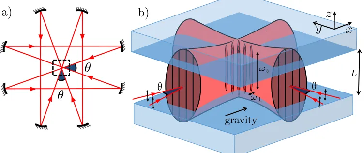
waves inxandy. This could be achieved with a pair of angled beams Nelson, Li, and Weiss,2007for each standing wave, in bow tie configuration [see Fig.1.6].

✓ ✓

!_?

gravity

L

b)

!z

a)

✓

✓

x

y

z

Figure 1.6: Layout of suggested experimental implementation. a) The beam con-figuration is achieved using a bow tie arrangement (view from above). Two pairs of beams are aimed at a vacuum chamber. In each pair, the two beams have a difference in k vector direction of θ = 30o, causing an in-plane standing wave to form in the direction perpendicular to that pair’s netk vector direction. The pair of perpendicular standing waves forms an attractive lattice. b) The two-dimensional lattice of attractive-potential tubes forms with transverse vibrational frequencyω⊥ and lattice constant ∆x. The finite beam width results in a weak potential in the

z direction with vibrational frequencyωz. Gravity is in the beam plane to avoid a potential gradient along the tubes. Blue-detuned light outside the central region of width L forms caps for the tubes. We obtain ω⊥ ' 2π ×10 kHz, ∆x ' 3 µm,

ωz '2π×100Hz, andL'10µm.

An additional blue-detuned optical potential at 394 nm, the Sr blue magic wave-length, is applied to form approximate 1D square wells from the resulting tubes. The potential could be formed from a projected image of a Gaussian beam with waist 30µm and total power 400 mW screened in the center by a rectangular mask of widthL= 10µm. Imperfect cap potentials, along with a finite curvature of the flat potential, contribute to∆U and are analyzed below.

over the use of unentangled atoms.

To observe spin diffusion, the most straightforward way of preparing the initial state and measuring observable Qˆ involves cooling a spin-polarized system to the limit where the lowestnorbitals are occupied. One could also potentially consider taking advantage of large N for better cooling Hazzard et al., 2012; Taie et al., 2012. One can then address different orbitals either spatially with spin-changing pulses which only couple to certain orbitals (for example using pulses focused on the center of the well and hence decoupled from orbitals that vanish there), or energetically by temporarily transferring atoms to another electronic state subject to a different potential. To observe spin diffusion with thermal atoms, one could rely on the fact that about half of the occupied orbitals are odd, and the other half are even, which becomes statistically more accurate for largern. It is possible to address only the even orbitals by using a beam focused at the center of the well, since the odd orbitals vanish there. This could be extended to largerN by using additional beams focused on other points in the well.

The bow tie configuration build-up cavity of attractive magic-wavelength (λ =813 nm) beams shown in Fig.1.6results in orthogonal standing waves in thex-yplane, whose intensity maxima are spaced by ' 3 µm, with beam waist of 100 µm at the intersection of the two beams. The build-up cavity will increase the beams’ intensity by a factor of ∼ 100 with a circulating power of 25 W. The resulting 1D trap sites have ω⊥ ' 2π×88kHz for the initial loading and cooling phase of the experiment. The (much weaker) longitudinal trapping frequency that results is

ωz '2π×880Hz.

The additional blue-detuned optical potential at 394 nm, the Sr blue magic wave-length, creates sharp caps on the resulting tubes. This potential could be formed by a projected image of a Gaussian beam with waist 30µm and total power 400 mW screened in the center by a rectangular mask of widthL= 10µm.

The large ω⊥ enforces a pseudo one-dimensional system as only the lowest ra-dial energy level will be populated. However, the desired condition that U =

Imperfections on the mask that creates the flat potential and imperfect edges of the trap from the blue-detuned potential contribute to∆U. In Section1.4we give an analytic bound that a harmonic perturbation of frequencyωz small enough that

M ω2

zL2 < ~

2_π2

M L2 leads to ∆U/U < 10−2. Exact diagonalization of the 1D potential

confirms that ∆U/U is even less sensitive to ωz: our parameters correspond to

M ω2

zL2 ≈ 750 ~

2_π2

2M L2, yet ∆U/U remains below one percent. The imaging system

used to form the potential contributes much more significantly to ∆U. With an imaging point spread function of full width at half maximum (FWHM) of 1 µm with atoms at 1µK, exact diagonalization results in∆U/U .5%.

Therefore with these parameters, one obtains U/~ = (4πaggω⊥)/L ≈ 2π ×10 Hz, and should be able to meet all three of the key requirements stated above with .20atoms in a single tube. In addition, as the pulses in the GHZ protocol should resolveU, they should have a sufficiently long duration 0.1s. With additional effort, it should be possible to reach a regime of higherU andn while satisfying these requirements. By shaking the trap during preparation with frequencies low enough to depopulate the lowest m energy orbitals, the restrictions on L and ω⊥ from the requirement that U = (4πagg~ω⊥)/L < 3~2(π/L)2/M is relaxed to

(4πagg~ω⊥)/L < [(m+2)2−(m+1)2]~2(π/L)2/M. Decreasing the ratio between the spatial imperfections of the potential andL will reduce∆U/U. For example, reducing the FWHM of the point spread function in our numerical calculations described above from 1µm to 0.5µm yields∆U/U <2%. Approaches for creating subwavelength potentials can also be envisioned Jendrzejewski,2014.

is negligible, while vector shifts can be avoided with the use of linear polarization. Specifically, to ensure any breaking of the SU(N) symmetry is far below a level which could affect our proposal, beam circularity of below a few percent should be sufficient. An appropriate choice of linear polarization of the blue-detuned beam will ensure minimal longitudinal field components (and hence minimal circularity) induced by imaging the mask.

1.11 Outlook

The proposed system opens a wide range of research and application avenues beyond those discussed above. For the case of N = 2, our Sn × SU(N)-symmetric Hamiltonian can be used for decoherence-resistant entanglement generation A. M. Rey, Jiang, et al., 2008, a method whose generalization toN > 2we postpone to future work. Furthermore, by comparing with the exact solutions presented here or those derived in the limit of strong interactions Volosniev et al.,2015; Deuretzbacher et al.,2014one could verify the performance of the proposed experimental system as a quantum simulator. The system can then be used to reliably study more general regimes where complexity theory might rule out efficient classical solutions. In particular, deviations from the square-well potential will breakSn[but notSU(N)] symmetry. This will for example lift the degeneracy of the most antisymmetric spin state (highest energy eigenspace forU >0). Depending on how this degeneracy is lifted, exotic many-body states might arise Miguel A Cazalilla and Ana Maria Rey, 2014; A. M. Rey, A. V. Gorshkov, Kraus, et al.,2014.

C h a p t e r 2

SPECTRUM ESTIMATION

In Chapter1, we studied an atomic system which gives rise to a highly symmetric nu-clear spin Hamiltonian which is decoupled from the spatial degrees of freedom. The decoupling arose because the trap used forces the Hamiltonian to have parameters which are symmetric under exchange of spatial states.

In this chapter, we argue that standard Ramsey spectroscopy on this system, enabled by its’ high symmetry, provides an efficient and accurate estimate for the eigenspec-trum of a density matrix whosen copies are stored in the nuclear spins ofn such atoms.

2.1 Motivation and Background

groupSn] and arbitrary simultaneous rotations [symmetry group SU(N)] of all n copies. Indeed the EYD algorithm simply projects the initial state onto irreducible representations ofSn×SU(N).

The best known strategy for spectrum estimation without joint measurements, is an adaptive two-stage protocol in which an asymptotically vanishing fraction of the copies are used with full tomography to estimate the eigenbasis of the state, which is used as a measurement basis on the remaining copies Ballester,2006. It is unclear if this strategy has the same sample complexity as the EYD strategy, but the author argues to be asymptotically as good under a different notion of performance. In any case, for the overhead involved for moderate numbers of copies could be prohibitive in practice.

However prohibitive the number of copies required for spectrum estimation using separable measurements, one may expect that the difficulty involved in making joint measurements of many quantum systems renders the EYD scheme highly impractical. Here we show that, surprisingly, Ramsey spectroscopy of fermionic alkaline-earth atoms in a square-well trap naturally performs the highly entangled EYD measurement onn copies ofρˆstored in thed-dimensional nuclear spin of n such atoms.

one manipulates the electron Childress et al.,2005; Reichenbach and I. H. Deutsch, 2007; A. V. Gorshkov, A. M. Rey, et al.,2009. Finally, this procedure can be used to characterize the entanglement of a given nuclear spin with others in a many-atom state obtained via evolution under a spin Hamiltonian Honerkamp and Hofstetter, 2004; A. V. Gorshkov, Hermele, et al.,2010; M. A. Cazalilla, Ho, and Ueda,2009; Miguel A Cazalilla and Ana Maria Rey,2014; X. Zhang et al.,2014; Scazza et al., 2014; Cappellini et al.,2014; we would needncopies of the many-atom state.

2.2 Overview of the proposal

As illustrated in Fig.2.1(a), to estimate the spectrum ofρˆ, whosencopies are stored in the nuclear spins of n |gi atoms, we transfer all n atoms into a single infinite square well, with at most one atom per single-particle orbital.

As detailed in Chapter1, for sufficiently weak interactions, due to energy conserva-tion and the anharmonicity of the trap, then occupied orbitals of the well remain unchanged throughout the experiment and play the role of sites. Thanks to the decoupling of the N-dimensional nuclear spin from the electrons,s-wave interac-tions give rise to a spin Hamiltonian with nuclear-spin-rotationSU(N)symmetry A. V. Gorshkov, Hermele, et al.,2010; M. A. Cazalilla, Ho, and Ueda,2009. Fur-thermore, the interaction strength between square-well orbitals labeled by positive integers p 6= q is proportional to R₀πdxsin2(px) sin2(qx) = π/4and is thus inde-pendent ofp andq, giving rise to the site-permutation symmetrySn beverland16 The resultingSn×SU(N)symmetric Hamiltonian,

ˆ

H =UX

j<k

(1₋sˆjk), (2.1)

is therefore diagonal in the EYD measurement basis, naturally turning Ramsey spectroscopy of this system into an implementation the EYD algorithm. As in Chapter1,sˆjk swaps spinsjandk, and the sum is over occupied orbitals. Here, we have explicitly restored the constantU n(n−1)/2which was omitted in Equation1.2

as it will be relevant here.

To include the first excited electronic state, one should use the prescription of Section1.7. For simplicity, we instead make the modeling assumption that atoms only interact if they are in the ground electronic state, such that the Hamiltonian is

ˆ

H_D =UX

j<k

ˆ

σ_ggj σˆk_gg(1−sˆjk)−δ

X

k

ˆ

whereσggj projects the atom in thejth orbital into the ground electronic state, andδ is an energy offset of the electronically excited level. This Hamiltonian would occur for particular (unrealistic) values of the scattering constants, or could be enforced by using different traps for the ground and excited electronic states, such that the density in the confined directions is much lower for atoms in the excited (rather than ground) electronic states.

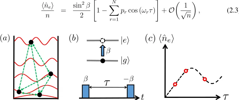
At the start of the Ramsey sequence, the initial state of the n-atom system is |GihG| ⊗ρ⊗n, where|Gi = |g . . . giand each nuclear spin is in the same stateρˆ. The first Ramsey pulse of areaβ between|giand|ei[Fig. 2.1(b)] is implemented over short timetP =β/Ω(so that interactions can be ignored), using Hamiltonian

ˆ

HP = Ω₂ P_k ˆσkeg+ ˆσgek

with Rabi frequency Ω and σˆµνk = |µikhν|. Then the system is allowed to evolve underHˆDfor a dark timetD. After the second Ramsey

pulse of area−β, the state is

ˆ

ρ0 = ˆU_p†UˆDUˆp|GihG|ρˆ⊗n( ˆUp†UˆDUˆp)†,

where Uˆp = exp[−itPHˆP] and UˆD = exp[−iτHˆD]. Finally, the number of |ei atomshnˆei=Tr[ˆneρˆ0]is measured, wherenˆe=Pjσˆee. We will show below thatj

hnˆei

n =

sin2β

2 "

1− N

X

r=1

prcos (ωrτ)

#

+O

1

√

n

, (2.3)

t

⌧

(

a

)

(

b

)

(

c

)

⌧

|

g

_i

|

e

_i

h

n

ˆ

i

Figure 2.1: Optimal spectrum estimation with alkaline-earth atoms. (a) n copies of anN-dimensional density matrixρˆare stored in the nuclear spin ofn fermionic alkaline-earth atoms trapped in the same square-well trap and prepared in their ground electronic state |gi. (b) A Ramsey sequence is applied consisting of two pulses of area β and −β, respectively, coupling |gi to the first excited electronic state |ei. (c) The numberhnˆei of |ei atoms is measured for O(N) different dark timesτ (red circles) between the pulses and allows to extract the eigenspectrum of

ˆ

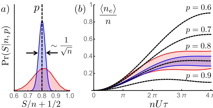
whereωr =U n(1−pr) cos2 β₂ +δ and(p1, p2, . . . , pN)is the eigenspectrum ofρˆ, ordered for future convenience asp1 ≥ p2 ≥ · · · ≥ pN. Moreover, asn increases, the distribution of measurement outcomes ˆne/n becomes tightly peaked about its expectation value hnˆei/n. As the measurement destroys ρˆ, we envisage starting withO(N)sets ofnatoms, each with nuclear spin stateρˆ. Performing the Ramsey protocol on each set for different timesτ [Fig. 2.1(c)] and comparing to Eq. (2.3) allows one to infer the spectrum ofρˆ. Notice an important difference from the usual Ramsey spectroscopy where the entire hˆnei curve as a function of τ is typically measured and each point on the curve requires many measurements.

The limiting cases of Eq. (2.3) make sense. Indeed, Rabiπ-pulses (β =π) give zero sinceHˆD → −nδ, soUˆp†UˆDUˆp = exp[inδτ]. Similarly,hnˆei = 0in the absence of Rabi pulses (β = 0) since no|eiatoms are ever created. Ifρˆdescribes a pure state, in which case one of thepr is unity while the rest vanish, the interaction U drops out (as it should for identical fermions) and we recover the familiar non-interacting expression. Whenρˆis maximally mixed, the system behaves as a non-interacting system with a frequency shift −U nN_N−1cos2 β₂. When N is large and allpr 1, the system behaves as a non-interacting system with a frequency shift−U ncos2 β₂.

2.3 Spectrum estimation forN = 2

To describe the physics behind our Ramsey-based spectrum estimation protocol and behind Eq. (2.3), we start by reviewing the original EYD spectrum estimation algorithm for the familiar case of qubits (N = 2, or, equivalently, spin-1/2). The algorithm states: Letting(p,1−p)withp≥1/2be the spectrum ofρˆ, in the limit

n_{→ ∞}, a single measurement onρˆ⊗nof the total spinSˆ2 [with possible outcomes

S(S + 1) with nonnegative S = n/2, n/2−1, . . .] gives an outcome satisfying