using model reference adaptive control.
White Rose Research Online URL for this paper:
http://eprints.whiterose.ac.uk/79684/
Version: Accepted Version
Article:
Virden, D. and Wagg, D.J. (2005) System identification of a mechanical system with
impacts using model reference adaptive control. Proceedings of the Institution of
Mechanical Engineers, Part I: Journal of Systems and Control Engineering, 219. 121 -
132. ISSN 0959-6518
https://doi.org/10.1243/095965105X9533
Reuse
Unless indicated otherwise, fulltext items are protected by copyright with all rights reserved. The copyright exception in section 29 of the Copyright, Designs and Patents Act 1988 allows the making of a single copy solely for the purpose of non-commercial research or private study within the limits of fair dealing. The publisher or other rights-holder may allow further reproduction and re-use of this version - refer to the White Rose Research Online record for this item. Where records identify the publisher as the copyright holder, users can verify any specific terms of use on the publisher’s website.
Takedown
If you consider content in White Rose Research Online to be in breach of UK law, please notify us by
System identification of a mechanical system
with impacts using model reference adaptive
control
D. W. Virden∗ and D. J. Wagg
Automatic Control Laboratory, Department of Mechanical Engineering, University of Bristol, Queens Building, Bristol BS8 1TR, UK.
Abstract
A single degree of freedom mechanical spring-mass system was considered
where the motion of the mass is constrained by an adjustable rigid impact stop.
A model reference adaptive control algorithm combined with interspike interval
techniques was used to consider the viability of identifying system parameters
when impacts are present. The unmodified adaptive control algorithm
desta-bilizes during vibro-impact motion, so three modified control algorithms were
tested experimentally. The first, thegain reset, was found to be of limited use
and system identification cannot be successfully carried out. The second and
third used again pause strategy. The second algorithm usedacceleration
trig-gering and represented an improvement on thegain reset method. The third
approach useddisplacement triggering and was found to be partially successful
in identifying system parameters in the presence of vibro-impact motion.
Keywords: Adaptive control, system identification, vibro-impact, interspike intervals.
Notation:
aij Element of plant matrix
A Plant matrix
Am Model plant matrix
Amd Discrete model plant matrix bi Element of controller matrix
B Controller matrix
Bm Model controller matrix
Bmd Discrete controller plant matrix b(t) Spike train time series
c Damping constant
H Spike train threshold
k Spring constant
km Controller constant
K Adaptive feedback gain
Kr Adaptive feedforward gain m Mass constant
r Reference signal
S Samples recorded during impact
ts Model settling time
u Control output
x Displacement of mass
˙
x Velocity of mass
xm Reference model displacement ˙
xm Reference model velocity xe System error
˙
xe Derivative of system error α MCS gain parameter
β MCS gain parameter
∆ Discrete sampling rate (samples/second)
1 INTRODUCTION
Systems with motion limiting constraints occur in many areas of mechanical en-gineering. For example, machines (Perterka & Kotera 1995), geared systems (Theo-dossiades & Natsiavas 2001, Karagiannis & Pfeiffer 1991), bearings (Neilson & Gon-salves 1993) and railway wheels (Knudsen et al. 1992). These types of systems present particular challenges in terms of mathematical modeling and control due to the nonlinear effects caused by impacts which occur during dynamic excitation.
Of the control techniques available, adaptive control allows a great deal of flexibil-ity when dealing with uncertain or time varying plant parameters, and for this work a model reference type adaptive controller was used with no prior tuning (Stoten 1993). The mechanisms for destabilization of MRAC controllers are well known; (Ioannou & Kokotovic 1984, Anderson et al. 1986), but systems with constraints present a particular challenge to developing a stable and robust adaptive control strategy (Zavala-Rio & Brogliato 2001, Tung, Wang & Hong 2000).
2 THEORETICAL FORMULATION
2.1 Control algorithm
In this work we use a model reference adaptive controller, known as the minimal control synthesis (MCS) algorithm (Stoten 1993). MCS is a form of model reference adaptive control that assumes no prior knowledge of the system parameters, and in which the adaptive control gains are all initially set to zero. We begin by considering the general linear state space formulation for MCS. The plant state equation can be written in the form
˙
x(t)=Ax(t)+Bu(t) (1)
wherexis the state variable vector of dimensionn×1,uthe control signal, dimension
p×1,A and B represent the linear dynamics of the plant.
The controller for the MCS algorithm is defined as
u(t)=K(t)x(t)+Kr(t)r(t), (2)
wherer(t) is the reference (demand) signal,K(t) is the feedback adaptive gain and
Kr(t) the feed forward adaptive gain. Substituting equation 2 into equation 1 gives
˙
x=Ax+B(Kx+Krr) = (A+BK)x+BKrr. (3)
This type of controller operates without explicit values for the matrices A and
B. Instead, the plant is controlled to follow the output of a reference model with known dynamics of the form
˙
xm(t)=Amxm(t)+Bmr(t), (4)
wherexmis the state of the reference model andAm andBmare linear reference
equivalents of A and B. For the experiments a discrete time approximation, xmd
was used as shown in Equation 5 using the parametersAmdandBmd from Equation
6
Amd=
1 ∆
−16∆/t2
s 1−8∆/t 2 s
,Bmd =
0 16∆/t2
s
(6)
The performance of the controller is monitored using the error signalxe=xm− x. The objective of the control algorithm is for xe → 0 as t → ∞. We can
reformulate the dynamics of the system as the error dynamics using x˙e =x˙m−x˙
such that
˙
xe=Amxe+ (Am−A−BK)x+ (Bm−BKr)r. (7)
Then providing (Am−A−BK) → 0 and (Bm−BKr) → 0 the stability of the
system will depend only on the matrixAm, which we can select in advance.
In general, the MCS gains are defined as
K= α
Z t
0
yex(t)dt+βyex(t) Kr = α
Z t
0
yer(t)dt+βyer(t)
(8)
where ye = Cxe, and C is chosen such that the transfer function C(sI−A)−1B
is strictly positive real (SPR) (Hodgson & Stoten 1996). The control weightings
α and β can be chosen to give the appropriate amount of adaptive effort. From empirical results we always maintain the ratioα/β= 10 andC= 4/ts(Stoten 1993)
(assuming first order control) wherets is the required settling time of the plant. The
MCS algorithm has been shown to be stable and robust for a wide range ofA and
B values (Hodgson & Stoten 1996; Hodgson & Stoten 1999; Stoten & Benchoubane 1990). Further details of implementing MCS for both first and second order systems can be found in (Stoten 1993).
2.2 System identification algorithm MCSID
The MCS control algorithm has been extended to a system identification algo-rithm by Stoten & Benchoubane (1993). The basic premise can be seen by comparing equations 4 and 3, from which we can see that for exact matching between the plant and the reference model, the following relations hold
A+BK=Am
BKr=Bm
Therefore it should be possible identify the unknown parameter matrices Aand
B by computing
B=BmK−r1
A=Am−BK
. (10)
assuming that K−1
r can be found (Stoten & Benchoubane 1993). The work carried
out in Stoten & Benchoubane (1993) relies on the system matrices,A andBhaving the following specific phase-canconinal form,
A=
A11 . . . A1p
..
. ...
Ap1 . . . App
, B=
B11 0
. .. 0 Bpp
, (11) where
Aii =
0 1 0 . . . 0
0 0 1 . . . 0
..
. ... ... . .. ...
0 0 0 . . . 1
−aii1 −aii2 −aii3 . . . −aiin i , (12) and
Aij=
0 . . . 0 ..
. ...
0 . . . 0
−aij1 −aij2 . . . −aijn j
, Bii =
0 .. . 0 bii . (13)
Here,ni is the state dimension of the ith degree of freedom, such that Ppi=1ni =n.
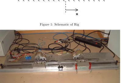
The reference model system matrices will have correspondingly similar structure. A schematic representation of the system is shown in Figure 1, from which we derive the equation of motion for the spring mass-damper system as
mx¨+cx˙+kx=kmu (14)
where x is the displacement of the mass and ˙x is the velocity. In this model km is
for the single mass rig. Writing equation 14 in a first order form gives ˙ x1 ˙ x2 = 0 1
−k/m −c/m x1 x2 + 0 km/m
u (15)
Thus we have a (2×2) A matrix and a (2×1) B matrix with the values
a21=−k/m a22=−c/m
b21=km/m
(16)
and a11= 0, a12 = 1, b11= 0.
2.3 Interspike intervals
Interspike intervals can be used to identify or reconstruct dynamic characteristics of a system from examining the intervals between a series of spikes or pulses (Sauer 1994). For impacting systems this can be applied to intervals between successive impacts (Wagg et al. 1999). A key requirement for interspike interval techniques is the accurate measurement of the spikes. Impulse spikes which occur in impacting systems with hard materials (e.g. steel on steel) are usually very short time events. The time of contact, τc, is related by S and ∆ such that τc ≈S/∆, where ∆ is the
digital sampling rate, and S is the number of samples recorded during contact. In this work we use an accelerometer attached to the impact stop (second algorithm) or displacement data (third algorithm) to produce aspike train signalb(t). Therefore we need a suitably fast sampling rate, ∆, to ensure that we capture spikes to a sufficient level of accuracy. However, spikes only occur for a very short time, at relatively large intervals, so a very fast ∆ will result in large quantities of unwanted data being recorded. We must also choose a suitably defined threshold value, H, to distinguish between spikes and noise. Thusb(t)> H is recorded as a spike, and
b(t) < H is disregarded. The choice of H is arbitrary, but must be made from inspection of a spike train signal. Failure to set an appropriate H value can lead to the following scenarios:
m
x
[image:9.595.146.449.107.234.2]k
impact stop [image:9.595.104.501.181.453.2]Figure 1: Schematic of Rig
Figure 2: Photograph of Experimental Setup
2. Threshold value too low; noise peaks may be mistaken for impulse spikes. These issues are discussed in detail in (Wagg et al. 1999)
3 EXPERMENTAL SETUP
system damping occurs due mainly to the friction in the track and gear system. These components also introduce some nonlinearity due to friction in the bearings on which the mass oscillates.
The system had an adjustable mass which allowed the weight of the trolley to be changed. For these experiments two configurations were used which weighed 0.75kg and 1kg respectively. The damping and spring constants remained unchanged for the duration of the experiment.
The impact stop was constructed from a piece of square metal block that was clamped to the track bed 45mmfrom the centre of the motor. 3mmof high density foam was attached to the end of the block. From the impact spike data, impacts were observed to last for approximately 1/15 of a second.
The position of the mass was controlled via an electric motor, and the displace-ment and velocity of the mass was recorded using a potentiometer and tachometer respectively. The signals are read via an Amplicon PC30AT card, which is also used to output the control signal. The control system was implemented on a 486 Personal Computer running RedHat Linux 5.1. A sampling rate of 256Hz was used for all tests. This was controlled using the Linux real time clock.
Preliminary tests were carried out on the rig to identify the nature of the damp-ing. This involved subjecting the rig to an impulse and observing the response. From these tests it was found that the system was close to critically damped,ζ ≈1.
For the work in this paper the MCS algorithm was implemented on the rig using the following parameters;α= 0.1,β = 0.01 andts= 1 second. The reference signal was composed of three sine waves
r= 0.4 sin(2πt) + 0.133 sin(3πt) + 0.08 sin(5πt). (17) This reference signal was chosen to satisfy the persistence of excitation condition (Sastry & Bodson 1989; Stoten 1993). The discrete reference model (Equation 5) was used with the discrete reference model parameters (Equation 6) with ts = 1s
and ∆ = 1/256s
-20 -10 0 10 20 30 40
0 50 100 150 200 250
Gain Amplitude
Time (s)
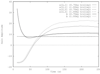
[image:11.595.123.469.96.351.2]a[2,1] (0.75kg trolley) a[2,1] (1.00kg trolley) a[2,2] (0.75kg trolley) a[2,2] (1.00kg trolley) b (0.75kg trolley) b (1.00kg trolley)
Figure 3: Non-impacting system parameters
The accelerometer was amplified using a customized DC amplifier and connected to an input channel on the Analogue to Digital Card (ADC). This signal was sampled at every control step and compared to the threshold to determine if an impact had occurred. The displacement spike train was computed from the displacement data and a predetermined threshold valueH.
4 EXPERMENTAL RESULTS
4.1 Non-impacting system identifcation
-2 -1 0 1 2 3 4 5
0 10 20 30 40 50 60 70
Gain Amplitude
Time (s)
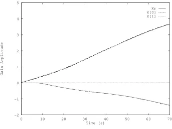
[image:12.595.126.469.96.355.2]Kr K[0] K[1]
Figure 4: Gain Values from Unmodified Algorithm
system are
a21=−k/m, a22=−c/m, b21=km/m (18)
wherekm includes the potentiometer, motor and amplifier gains.
The results of the two tests are shown in Figure 3. Data was recorded from approximately 10 seconds after the test started. From Figure 3 we see that the parameter values have stabilized after a further 200 seconds. This experiment was run twice, once with each mass configuration. Dividing the settled value of the a21
parameter for each trolley configuration gave a ratio of 0.723 which is very favorable when compared to the predicted ratio of 0.75.
-2 -1 0 1 2
0 5 10 15 20 25 30 35 40 45 50
Magnitude
Time (s)
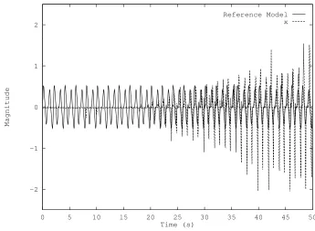
[image:13.595.122.467.97.350.2]Reference Model x
Figure 5: Displacement under Unmodified Algorithm
4.2 System identification with impacts
4.2.1 Unmodified algorithm
An initial test was carried out to see the effect of introducing an impact on the standard MCS control algorithm. For these tests Kr = kr is scalar and K =
[k[0], k[1]]T. The result of this test was that the control gains, k
r and k[0] were
found to increase steadily from timet= 0 in an approximately linear manner. This is shown in Figure 4, where we also note that gaink[1] remains at an insignificantly small amplitude throughout the test. The increasing gain phenomena is known as “gain wind up”, and will eventually lead to a sudden destabilization of the controller. In this example the mechanism behind the gain wind up is due to the introduction of a strong nonlinearity associated with the impact. In Figure 5 the displacement of the trolley under the unmodified algorithm is shown.
-2 -1 0 1 2 3 4 5
0 50 100 150 200
Gain Amplitude
Time (s)
[image:14.595.126.470.96.350.2]Kr K[0] K[1]
Figure 6: Gain Values from Gain Reset Algorithm
trolley moves and starts to impact. This can be seen in Figure 5 where the first impact occurs at approximately 27s with an amplitude of ∼ 0.45V. This regular
impact, with a period of 2s, represents a strong non linearity which causes further controller gain windup which will eventually cause the unmodified algorithm to lose stability. The motion of the trolley gets less predictable as the gains continue to windup and its velocity increases. This results in the increased displacement seen after 37s in Figure 5. The spikes which are greater than 0.45V are due to the high impact velocities, which occur during the loss of stability, where at each impact a significant impulse force is transferred to the experimental apparatus.
4.2.2 Gain reset algorithm
check for impact
no impact impact
wait until r<r(impact)
resume normal MCS
next timestep hold r wait for
[image:15.595.224.374.97.334.2]fixed time step
Figure 7: Schematic of Gain Pause Algorithm
For these tests an impact correlated to a spike of greater than the threshold value
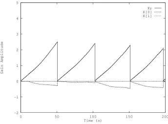
H= 2.3V from the accelerometer. The results from the test are shown in Figure 6, where we have plotted the control gains. Again we note thatk[1] is of such a small amplitude, that it is indistinguishable from the time axis. Although this approach proved successful in preventing gain wind up, it is very inefficient in terms of control, and could only be recommended if no other technique could be applied. It is certainly not suitable for application to a system with a periodic impact as the control suffers noticeably. However one potential application would be to implement the method as a safety mechanism, on systems where an impact is not normally expected. It is also clear from Figure 6 that system identification cannot be attempted using these results, as the gains do not have sufficient time between impacts to attain steady state values.
4.2.3 Gain pause algorithm
-10 -8 -6 -4 -2 0 2 4 6
0 50 100 150 200 250
Gain Amplitude
Time (s)
[image:16.595.123.475.97.349.2]Kr K[0] K[1]
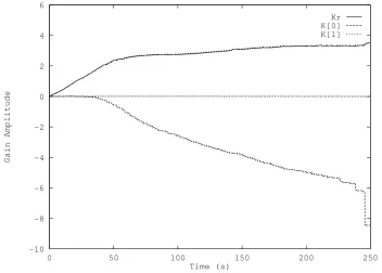
Figure 8: Gain Values from Gain Pause Algorithm (Acceleration Triggering)
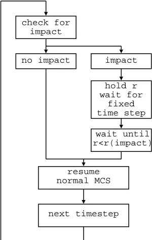
as before, and then pausing adaption, initially for a fixed interval of 0.25 seconds, and waiting until the reference signal had dropped below the value that had caused the impact. The reference signal was not allowed to resume the original function until it was less than the value that caused the impact. The fixed interval of 0.25swas used in order to prevent the switch between adaption, pause and back to adaption occurring too rapidly — it was noted during tests that rapid switching could cause controller destabilisation as essentially this is a form of nonsmooth event itself. A schematic flow diagram showing the complete gain pause algorithm is shown in Figure 7.
The MCS gain values computed during a typical test are shown in Figure 8. We note that as with previous examplesk[1] is of negligible amplitude. From Figure 8 we can also see that althoughkr reaches a steady state value, the absolute value ofk[0] increases steadily throughout the test, and has some step jumps in amplitude towards the final stages of the test. As a result, in this system, the system identification could only be carried out on theKr gain data. The step increases in thek[0] gain occurred
due to a series of missed impacts.
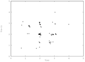
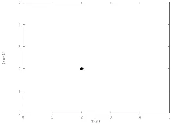
In Figure 9, we have plotted the (n−1)th interval between spikes, ∆Tn
0 1 2 3 4 5
0 1 2 3 4 5
T(n-1)
[image:17.595.124.471.97.350.2]T(n)
Figure 9: Interspike Intervals (Gain Pause, Acceleration Triggering)
the nth interval ∆Tn. For this test we see that the majority of impacts occurred at intervals of approximately 2 seconds. However, there are a range of other ∆Tn
values, which mean that the interspike interval plot forms a grid like pattern. This grid layout is indicative of a general problem of missing spikes or identifying spurious spike — both cases are discussed in detail in (Wagget al. 1999).
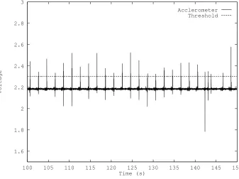
Figure 10 shows the threshold value, H, and the signal from the accelerometer used to calculate the interspike intervals.
4.2.4 Displacement triggering
1.6 1.8 2 2.2 2.4 2.6 2.8 3
100 105 110 115 120 125 130 135 140 145 150
Voltage
Time (s)
[image:18.595.121.471.115.674.2]Acclerometer Threshold
Figure 10: Spike Train and Threshold
-2 -1 0 1 2 3 4
0 50 100 150 200 250 300
Gain Amplitude
Time (s)
Kr K[0] K[1]
[image:18.595.130.467.116.368.2]0 1 2 3 4 5
0 1 2 3 4 5
T(n-1)
[image:19.595.122.468.97.351.2]T(n)
Figure 12: Interspike Intervals (Gain Pause, Displacement Triggering)
is shown in Figure 11, where we have plotted the MCS gain values for a typical displacement triggering test. The interspike interval plot for this test is shown in Figure 12. This shows that the motion is dominated by an interspike interval of ∆t ≈ 2. This indicates a predominately period one vibro-impact motion (Bishop et al. 1998), and shows that the problems with missed/spurious spikes have been eliminated in this case.
Tests were run using the displacement triggering method with a 0.75kg and a 1kg trolley to determine if it was possible to use this algorithm for system identification (the figures show the results from the experiments using the 0.75kg trolley). The resulting gains were then used to calculate the system parameters. The ratio of the
a21 parameters (which corresponds to k/m, was identified. As k remains constant,
-0.5 0 0.5 1 1.5 2
0 50 100 150 200 250 300
Ratio
Time (s)
[image:20.595.130.469.116.368.2]Actual Theoretical
Figure 13: Ratio ofa2,1 Parameters
0 0.2 0.4 0.6 0.8 1 1.2
0 50 100 150 200 250 300
Ratio
Time (s)
[image:20.595.121.475.121.671.2]Averaged Value Theoretical Value
a21 was recorded and averaged over a 78s period after the gains had stabilized and
was found to be 0.6846. It was noted that the mean experimentally observed values for the system parameters tended to be lower than the predicted ones. The presence of large fluctuations is unavoidable, as we see from the adaptive gain plot in Figure 13. But taking a cumulative average over a period of time, Figure 14, shows the ratio converging to a steady value. Taking the averaged value across a suitably large steady state time range, we obtain estimated parameter values which are reasonably close to those predicted by theoretical calculations. This has been achieved using a modified linear adaptive algorithm in the presence of a strong impact nonlinearity which occurs at least once every forcing cycle.
5 Conclusions
In this paper a single degree of freedom spring-mass-damper experimental system was studied, which was subject to motion limiting constraints which led to impacts. The focus of this paper has been to determine if it is possible to carry out system identification of the system parameters, using adaptive control, in the presence of impacts. The unmodified adaptive control algorithm was found to destabilize via gain wind up in the presence of impacts. Three modified methods were investigated to try and improve this situation.
The first modified method used gain resetting after each impact. This stabi-lized the system, but did not allow system identification to be carried out. The second modified method used gain pausing at each impact. The gain wind up was still present and prevented system identification from being performed. The final modified method — based on displacement triggering — proved successful in both stabilizing the vibro-impact system, and in giving a estimation of the chosen system parameter with at least 80% accuracy.
Acknowledgments
References
Anderson, B. D. O., Bitmead, R. R., Johnson Jr, C. R., Kokotovic, P. V., Kosut, R. L., Mareels, I. M. Y., Praly, L. & Riedle, B. D. (1986). Stability of
adaptive systems: Passivity and averaging analysis. MIT press: Cambridge Massachusetts.
Annaswamy, A.M. & Wong, J. (1997). Adaptive Control in the Presence of Saturation Non Linearity.International Journal of Adaptive Control and Signal Processing 11, 3–19.
Bishop, S. R., Wagg, D. J. & Xu, D. (1998). Use of control to maintain period-1 motions during wind-up or wind-down operations of an impacting driven beam.Chaos, Solitons and Fractals 9(1/2), 261–269.
Hodgson, S. P. & Stoten, D. P. (1996). Passivity-based analysis of the minimal control synthesis algorithm.International Journal of Control 63(1), 67–84. Hodgson, S. P. & Stoten, D. P. (1999). Robustness of the minimal control
synthesis algorithm to non-linear plant with regard to the position control of manipulators. Preprint.
Ioannou, P. A. & Kokotovic, P. V. (1984). Instability analysis and improvement of robustness of adaptive control.Automatica 20(5), 583–594.
Karagiannis, K. & Pfeiffer, F. (1991). Theoretical and experimental investigations of gear rattling.Nonlinear dynamics 2, 367–387.
K´arason, S.P. & Annaswamy, A.M. (1994). Adaptive Control in the Presence of Input Constraints.IEEE Transactions on Automatic Control 39(11),
2325–2330.
Knudsen, C., Feldberg, R. & True, H. (1992). Bifurcations and chaos in a model of a rolling railway wheelset.Philosophical Transactions of the Royal Society of London A338, 455–469.
Control 43(4), 560–564.
Neilson, R. D. & Gonsalves, D. H. (1993). Chaotic motion of a rotor system with a bearing clearance. InApplications of fractals and chaos, A. J. Crilly, R. A. Earnshaw, & H. Jones (Eds.), 285–303. Springer-Verlag.
Perterka, F. & Kotera, T. (1995). Different ways from chaotic motion in
mechanical vibro-impact systems. InNinth World Congress on the Theory of Machines and Mechanisms, Volume 2, Politecnico of Milano, Itay.
Sastry, S. & Bodson, M. (1989). Adaptive control:Stability, convergence and robustness. Prentice-Hall:New Jersey.
Sauer, T. (1994). Reconstruction of dynamical systems from interspike intervals.
Physical Review Letters 72(24), 3811–3814.
Stoten, D. P. (1993). An overview of the minimal control synthesis algorithm. In
I. Mech. E. Conference on Aerospace Hydraulics and Systems, London. Paper C474-033.
Stoten, D. P. & Benchoubane, H. (1990). Robustness of a minimal controller synthesis algorithm.International Journal of Control 51(4), 851–861. Stoten, D. P. & Benchoubane, H. (1993). The Minimal Control Synthesis
Identification Algorithm.International Journal of Control 58(3), 685–696. Theodossiades, S. & Natsiavas, S. (2001). Periodic and chaotic dynamics of
motor-driven gear-pair system with backlash. Chaos, Solitions and Fractals 12, 2427–2440.
Tung, P-C., Wang, S-R. & Hong, F-Y. (2000). Application of MRAC theory for adaptive control of a constrained robot manipulator.International Journal of Machine Tools & Manufacture 40, 2083–2097.
Wagg, D. J., Karpodinis, G. & Bishop, S. R. (1999). An experimental study of the impulse response of a vibro-impacting cantilever beam.Journal of Sound and Vibration 228(2), 243–264.