Pipeline network features and leak detection by cross-correlation analysis of reflected waves

promoting access to White Rose research papers

White Rose Research Online

Universities of Leeds, Sheffield and York

http://eprints.whiterose.ac.uk/

This is an author produced version of a paper published in

Journal of Hydraulic

Engineering.

White Rose Research Online URL for this paper:

http://eprints.whiterose.ac.uk/9115/

Published paper

Beck, S.B.M., Curren, M.D., Sims, N.D. and Stanway, R. (2005)

Pipeline network

features and leak detection by cross-correlation analysis of reflected waves.

Pipeline Network Features and Leak Detection by

Cross-Correlation Analysis of Reflected Waves

HY/2001/00227878

SBM Beck*1 PhD FIMechE, MD Curren2 MEng AMIMechE,

ND Sims3 PhD MIMechE and R Stanway4 DPhil FIMechE

1

Corresponding author: [email protected]. Senior Lecturer, Department of Mechanical Engineering, The

University of Sheffield, Mappin Street, Sheffield, S1 3JD, UK.

2 _{Design Engineer, Rolls-Royce Plc, PO Box 31, Derby, DE24 8BJ, UK.}

3

EPSRC Advanced Research Fellow, Department of Mechanical Engineering, The University of Sheffield,

Mappin Street, Sheffield, S1 3JD, UK.

4

ABSTRACT

This article describes progress on a new technique to detect pipeline features and leaks using

signal processing of a pressure wave measurement. Previous work (by the present authors)

has shown that the analysis of pressure wave reflections in fluid pipe networks can be used to

identify specific pipeline features such as open ends, closed ends, valves, junctions and

certain types of bends. It was demonstrated that by using an extension of cross-correlation

analysis, the identification of features can be achieved using fewer sensors than are

traditionally employed. The key to the effectiveness of the technique lies in the artificial

generation of pressure waves using a solenoid valve, rather than relying upon natural sources

of fluid excitation.

This paper, uses an enhanced signal processing technique to improve the detection of leaks. It

is shown experimentally that features and leaks can be detected around a sharp bend and up to

seven reflections from features/leaks can be detected, by which time the wave has traveled

over 95 meters. The testing determined the position of a leak to within an accuracy of 5%,

even when the location of the reflection from a leak is itself dispersed over a certain distance

and, therefore, does not cause an exact reflection of the wave.

Keywords:

INTRODUCTION

With the ageing infrastructure of many cities, there has been a growing interest in the

development of leak location techniques for water distribution and sewerage collection

(Covas et al 2000). These developments have been driven by the environmental, economic,

and legal liability costs of pipeline leaks. In 1994, for example, an estimated 23% of the

potable water in the UK was lost in leaks and ruptures (Water Resources Council, 1994).

Traditionally, the condition of pipeline networks in water distribution systems and industrial

processes has been monitored by a distributed set of pressure sensors, flow meters and valve

sensors. Such sensing devices allow the state of the entire network to be monitored, from the

state of valves to the presence of blockages and leaks (Seborg et al 1989). One disadvantage

of this approach, however, is that multiple sensors are required to monitor a complex pipe

network. Consequently, a complex pipe network could require many tens or even hundreds of

distributed sensors. Also, this kind of monitoring is somewhat awkward as, for example

networks operating in hostile or inaccessible environments.

In conjunction with these monitoring and detection systems, a number of techniques have

been developed for leak identification. This is usually achieved by monitoring the flow rate

through various zones of the network. The extent of a zone is then reduced by closing valves

and re-monitoring flow. Eventually, the pipeline branch where the leak is located can usually

be determined. This method relies on the availability of a sufficient number of valves and

flow meters in the system (i.e., an over-determined problem (Liggett and Pudar 1992), and on

the accuracy of the flow measurement.

A number of methods have been developed to assist with leak location process, for example

Susu 2004). Once a faulty pipeline branch has been located, the leak’s position must be

accurately determined. Current techniques include acoustic methods, tracer injection, video

inspection (Liggett and Chen 1994), and focused electrodes (Gokhale and Graham 2004). A

simple acoustic method uses a stethoscope to listen to the noise generated from a leak, success

being dependent upon the operator’s experience, the size of the leak, and the characteristics of

the pipeline and surrounding terrain. Alternatively, acoustic sensors can be used to detect

leaks (rather than locate them) by listening for the characteristic sounds. However, both

acoustic and non-acoustic methods require significant levels of expertise and effort, and the

water supply typically interrupted. Currently when performing leak detection or location, the

effects of other legitimate pipeline disturbances, such as domestic and industrial water usage,

must be minimized. Consequently, the process is usually carried out at night.

From the above overview, it is clear that there is ample scope for the development of

improved solutions to the leak detection problem. In this paper, recent progress is described

concerning a novel technique for pipe network analysis. Although the technique is still some

way off from the practical implementation described above, it is shown in laboratory

experiments that the technique is effective in identifying the location of pipeline features

(junctions and bends) and leaks.

The proposed approach relies on signal processing techniques that are applied to

measurements of pipeline pressure. Similar concepts were used by Mpesha et al (2001), who

reported that measurements of flow and pressure variations at a single point can be used to

generate frequency response functions that help to ascertain the position and size of a leak in

branched systems. Liou (1998) used cross-correlation techniques to find the position of a leak

in a pipeline from the first reflection of a pressure wave from the leak. Taken together, these

results indicate that it is feasible to use signal analysis techniques to obtain valuable

This work represents a continuation of the investigations and modeling work of Beck and

various colleagues (Beck et al, 2000, and 2002). Here, the features of a pipe network were

detected using an artificially generated pressure wave along with a single pressure transducer,

and the signals were analysed using an extension of cross-correlation methods. In Beck et al,

(2000), the reflections from a known pipe network were modeled using the Transmission Line

Modeling (TLM) technique that had been developed previously by Beck et al, (1995). A

computer program was then used to cross-correlate the stimulus and response signals, and it

was shown that the cross-correlation technique was capable of detecting reflections and hence

of identifying key features in pipe networks. This work used the second derivative of the

cross-correlation multiplied by the time interval to produce clearly defined peaks showing the

position of reflection points. In comparison, the work reported by Liou (1998) focused on the

first reflection of the pressure wave and did not perform differentiation of the cross-correlated

signal.

Beck et al (2002), then performed experiments on an equivalent pipe network which was

constructed in the laboratory. The analysis was performed using the cross-correlation facility

of a commercial signal analyzer. The main factors that made the results difficult to analyze

were the accuracy with which the speed of sound was known and reflections at even large

radius bends. However, it was shown that the technique could identify the reflection points in

a real fluid network. The chief conclusion was that correlation analysis could be applied to

practical situations, but that there were several factors that affected the accuracy of the

process. For example, double differentiation of signals is undesirable owing to the tendency

of the operations to amplify noise.

The current work extends this experimental work through the use of improved data analysis

THEORY

When fluid flow (liquid or gaseous) in a pipe is suddenly stopped by a valve, pressure waves

are created. These waves travel along the pipe until they reach a feature of the pipe network,

where the wave is usually partly transmitted, and partly reflected back towards the source.

Some of the wave energy is inevitably absorbed by the feature in the form of a pressure loss

(Lighthill, 2001).

A pressure transducer can detect this pressure signal as the wave first traverses it and then

again as it returns after having been reflected. If the speed of the wave c in the fluid is known,

and the time t between the two passes of the wave at the pressure transducer is recorded, then

the distance l to the point of reflection is half the product of the wave speed and the travel

time.

2

t c

l= × (1)

The speed of the wave in the fluid can be found from many texts (Thorley 2004). It should be

noted that these equations are only true for single phase fluids in rigid pipes. If the pipe is

flexible or the fluid is multiphase, the speed of sound can be dramatically lowered.

The pressure wave carries even more information, as some features in the pipe network will

cause a reversal of the wave polarity. Knowledge of such shifts in polarity give an indication

of the cause of the reflection. This information, however, is not directly available from

observation of the pressure trace itself, since the pressure wave develops over a period of

time. As such, if the pipe network has many features that cause reflections, then some of the

pressure waves are likely to overlap, making identification difficult or even impossible. To

overcome this problem, suitable signal processing techniques are helpful for obtaining

Cross-correlation Techniques

Signal processing techniques such as cross-correlation are well established in engineering

applications (Lange 1987). Cross-correlation is used to recognize specific patterns in a signal

by comparing the signal, x, to a reference template, y. The data from each signal is

represented as an array, containing N elements of data, x

[ ] [ ]

[ ]

[ ] [ ] [ ]

The value r

[ ]

[ ]

∑

[ ]

[

]

−∞ =

+ × =

n

k n n

k x y

r (2)

In practice, measured signals have a finite length and so the sum in equation 2 is limited to the

range 0<n<N. A series of different values of r[k] is produced for increasing integer values of

k. Increasing k effectively moves the signals over each other, and the summation produces a

value indicative of how well the two signals match up, or correlate.

The computation starts with a time shift of k =0 and then k is increased incrementally up to a

suitable integer value. This procedure is equivalent to multiplying the overlapping elements of

the two signals, and summing with appropriate time shifts. When peaks within the same

signal overlap, however, the peaks of the cross-correlation are effectively added together to

create a different single peak with changing gradients. The peak of the second signal

corresponds to a change of gradient of the peak of the cross-correlation so, to find this peak,

the cross-correlation can be differentiated twice. The first differential indicates the magnitude

of the gradients and the second differential exhibits peaks at the points where the gradient

changes. Therefore the points at which the peaks occur on the graph of the second differential

are indications of reflected waves. This procedure is described more fully with examples

IMPLEMENTATION

In previous work (Beck et al 2002), the cross-correlation process was performed using

dynamic signal analyzer hardware. This posed some key problems as the signal processing

capabilities were somewhat limited. First, the hardware did not enable double-differentiation

of the cross-correlated signal. Second, the signal y[n] was obtained from the voltage signal

sent to the solenoid valve, so that the dynamics of the solenoid valve contaminated the results.

Finally, the data averaging techniques that could be used were limited.

In the present study, a new implementation of the signal processing was developed. A

data-logger based upon the Matlab dSPACE system was used (dSPACE, 2003), so that the data

could be recorded directly into a MATLAB environment (Mathworks, 2004).

Cross-correlation can be readily performed using MATLAB (Denbigh, 1998) due to its ability to

work with large matrices. This allowed the implementation of the following signal processing

method:

1) The first step was the automatic actuation of the solenoid valve (used to generate the

pressure wave), and acquisition of the corresponding pressure measurement. This

could be performed directly from the personal computer, with appropriate Matlab

programming.

2) To reduce the noise, the solenoid actuation and data acquisition was repeated a

number of times, M, and the average pressure measurement obtained. A short

convergence test was conducted to characterise M. For these networks, the average of

16 traces was used to smooth out the data points without unduly increasing the amount

of data.

[ ]

∑

[

]

This had the greatest effect in reducing noise and smoothing out the signal, making it

more suitable for differentiation. A consequence of this averaging was that some of

the data is lost. However, without the running average, the variation between one data

point and the next was sufficiently large to render results of the cross-correlation,

especially after double differentiation, very noisy.

4) The data was now de-trended by removing its mean value. This was a necessary step

to ensure correct results from the cross-correlation function.

5) To avoid contaminating the results with the effects of the dynamics of the solenoid

valve, an alternative to the solenoid voltage signal) was used for y[n]. Ideally, y[n]

should represent the initial pressure wave produced by the valve. Consequently, this

signal was generated by using the appropriate part of the signal x[n] corresponding to

the pressure wave and not the reflections. Mathematically:

[ ]

[ ]

∑

where p1 and p2 define the start and end points of the initial pressure wave. These were

determined graphically from a visual analysis of the signal x[n].

6) Finally, cross-correlation was performed on the signals x[n] and y[n], using

equation 2. The resulting signal was differentiated twice, giving:

[ ]

[ ]

[

]

∆t 1 k k

k = r −r −

and

[ ]

[ ]

[

]

∆t 1 k k

k = r −r −

r&& & & (7)

where ∆t is the sample time for the data acquisition system. The signal r&&

[ ]

plotted against the product of the measurement number (n), speed of sound of the fluid

(c) and sample time (∆t) on the ordinate, representing the distance traveled by the

wave.

In summary, a key contribution of this paper is the development of a signal processing

routine, based in Matlab, to implement the proposed theoretical approach. The application of

this routine will be demonstrated experimentally, to identify both leaks and pipeline features

such as bends and junctions.

EXPERIMENTAL PROCEDURE

The experimental pipe networks used in the present work consisted of 15 mm

outside-diameter copper pipe (see Figure 1). The working fluid used was air from an adjustable

high-pressure line. The high-pressure was set at approximately 1 bar (the exact value does not affect the

results). The air supply was connected to the copper pipe network via a rubber hose, which

caused high attenuation so that any waves that entered from the air supply could be neglected.

The output from two pressure transducers was electronically amplified before it was recorded

by the dSPACE data acquisition system. The solenoid was normally closed, and was driven

by a signal generator that produced a square wave with a frequency of 0.5 Hz. The system

trigger was set to monitor the input to the solenoid valve and started recording the traces on

the rising edge of the solenoid signal (when the valve was in the act of closing). A sampling

corresponding spatial resolution of the system was 3 cm, which was sufficient to determine

the origin of any significant reflections.

Once the pipe network was assembled, the relevant taps were open or shut as required. After

opening the high-pressure air valve, the system was allowed to run for several minutes to

attain steady state, at which time the computer was set to record. After sixteen traces had been

recorded, the computer was stopped and the equipment shut down if no more traces were

required. The Matlab script was then run using the newly acquired data, and the various traces

were studied. Each trace was recorded for 1.6 seconds, which represented the longest run that

the monitoring system would allow.

To determine the distance the reflections had traveled required knowledge of the speed of the

pressure wave. However, when this value was based upon that for air at ambient temperature,

it was found to give incorrect results, with the speed of sound 1.5% too low. Reverse

calculation from an earlier set of results gave an effective temperature of 6°C. This

temperature is lower than the laboratory air supply and is almost certainly due to the elasticity

of the pipe causing a decrease in the speed of sound (Massey 1979), implying that when

calibrating the system, the temperature appears too low. Adjusting the wave speed greatly

increased the spatial accuracy of the analysis.

EXPERIMENTAL RESULTS

Although the authors have conducted many experiments, only a small sample are described

here. The first consists of a straight pipe with a straight section at right angles added to it and

with a tap on the end; effectively a half T-junction as shown in Figure 1. The next two pipe

networks use the same arrangement, but runs were made both with and without holes in order

Analysis of Half T-junction Network

The initial analysis was conducted with both the tap near the T-junction (node 5) and the tap

at the end of the pipe (node 7) open. The main paths that were expected to be produced are

shown in Table 1. The pressure data were obtained using a pressure transducer that was

situated 2.16 m from the solenoid valve (node 2).

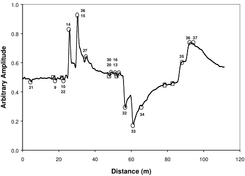
Figure 2 shows the result of this experiment (after cross-correlating, double differentiating

and calibrating the abscissa in meters). With reference to Figure 2, the circles numbered 1 to 8

indicate the peaks where the distance and polarity corresponded to a predicted reflection of

the pipe network. The paths corresponding to these peaks are shown in Table 1. It is clear that

some of the peaks are straightforward to discern, whereas others would not be spotted if the

physical arrangement of the pipe network was not known beforehand. Using this technique,

even though it is possible to identify features that are already known, it would be difficult to

identify the physical analogies of the peaks for a system whose lengths and features are not

known.

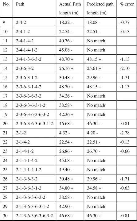
The test was now repeated with tap 5 shut and tap 7 open and after processing, the paths

identified. The peaks were marked with black circles in Figure 3. The relevant paths are

outlined in Table 2 which contains the data for all the different possible paths up to a

maximum length of 50 m. Where a peak matches up with a path, the predicted path length and

measured path length, along with the percentage error, are stated. The "+" symbol indicates a

positive peak, and the "–" symbol indicates a negative peak. It can be seen that 13 out of the

22 possible paths were identified, although some of the peaks in Figure 3 were not strongly

defined, for example those for paths 20, 23 and 30. In each case, the relevant peak was

adjacent to a peak of much greater magnitude of the opposite orientation. Some of the paths

listed in Table 2 represent the same length and orientation, as they are the same routes, but in

A number of paths over 50 m in length are shown in Table 3. As there are too many possible

combinations to list, only the possible paths for the peaks actually found in Figure 3 are

included.

To summaries the results from this experiment, the first large positive peak, corresponding to

path 14 detected a reflection from the open tap at node 7. A repeat reflection from this point

was found (path 15) which was the second largest positive peak. A second order reflection

from this tap was then found (path 32) which was again repeated (path 33), and can be

identified as the two prominent negative peaks. A third order reflection (path 35) which was

again repeated (path 36) was also found, but the peaks were not as well defined.

Double reflections from the closed tap at point 5 were found (paths 9 and 10) and these were

also repeated (paths 13 and 30), but no further reflections of this wave were detected. The

reflection from the solenoid valve at point 1 was also detected (path 21), as were the second

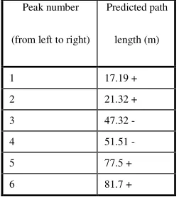
(path 27), third (path 34) and fourth (path 37) reflections. The peaks surrounded by a square

could not be attributed to any particular path, but their distances are listed in Table 4. These

results seem to indicate that a reflection originating at a measured distance of 8.6m was

detected, and then further repeat reflections of it were also detected. This reflection

corresponds to four times the distance between the valve and the pressure transducer (2.16 m),

though it is not known how large a reflection is caused by the transducer and mount.

Half T-junction with a Leak

In order to ascertain whether the technique can be used to detect leaks, a hole was introduced

into the half T-junction network shown in Figure 1. A 4 mm diameter hole was drilled in a

small length of pipe and the pipe section was inserted into the network this is node 3.

and this case is shown as the denser trace in Figure 4. Using the same pipe network, but with

the hole open at node 3, the analysis is shown as the thinner black trace in Figure 4. The linear

distances of the major peaks from the solenoid are shown numerically in Table 5 and Table 6.

It can be seen from Figure 4 that two clear new peaks (58 and 59) have been produced

through the opening of the hole. The first of these is at 11.48 m which corresponds to a direct

reflection from the hole. The second of these (at 15.78 m) can be identified as a double

reflection from the hole and then the valve. The hole is thus a new reflection point and its

position can be found.

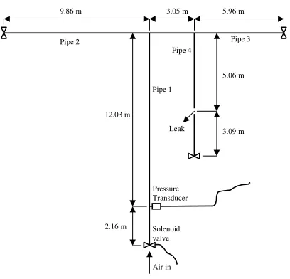
Leak Detection in a More Complex Network

A larger network was then set up in the laboratory (Figure 5 and Figure 6) which contained

four pipes, joined by three junctions. A 4 mm hole was drilled 22.3 m from the solenoid. It

was possible to cover and uncover this hole using tape. To reach the leak, the wave had to

traverse two right angle T-junctions.

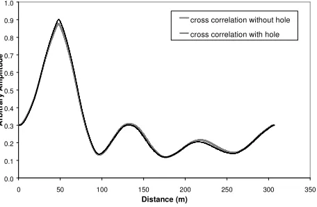
Pressure traces recorded with and without the hole are shown in Figure 7. It is seen that the

difference between these traces is almost indiscernible as was the cross-correlation signals

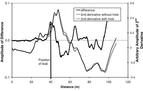
(Figure 8). The second derivatives of the cross-correlations multiplied by the time step are

shown in Figure 9, along with the difference between them. By this stage in the processing, it

is possible to tell the difference that the hole in the pipe has made to the response. A new peak

is visible at about 43 m and the negative peak seen which could be seen at 38 m on the trace

without the leak is no longer apparent. Many of the other reflection points, such as those at

24, 28 and 32 meters are also identified on this plot.

If the technique were to be used on a pipe network to find whether or not there were leaks,

providing that the lengths of the pipes in the network were known, the two new characteristic

characteristic lengths should correspond to one of the pipes in the network, indicating in

which pipe the leak is located.

The effect of the leak is clearly seen on the difference graph shown in Figure 9. There are no

differences up to about 37 m, but after this, this line starts rising to a peak at about 40 m. This

distance corresponds to twice the distance between the leak and the pressure transducer, with

a 5% error. There are other features that can be discerned from the difference graph. The peak

at 43 m is the reflection of the leak from the valve just downstream of it. There is another

peak at 56 m which is the reflection from the leak via pipe 3.

Additional experiments were conducted using a 6 mm hole in the pipe. Using the differencing

techniques described above it was also possible to detect these. Surprisingly, this gave a

slightly less distinct peak, probably due to the fact that the reflection was caused over a longer

distance. This might be explained by the fact that the leak is a hole that is parallel to the

direction of the pressure wave, so it does not represent a discrete position for reflection of the

wave. Work is continuing to measure the response of different sizes of holes, with a view to

identifying the size of a leak.

DISCUSSION

It stands to reason that that the greater the reflection length, the less prominent are the peaks

on the graph. This result is partly due to attenuation of the pressure wave. Some techniques,

such as acoustic methods, require information regarding the amplitude of the wave in order to

carry out the analysis. One of the greatest advantages of the cross-correlation technique is that

it does not require information about the amplitude of the pressure wave in order to function.

The single criterion is that there is a discernible amplitude, which can then be used in the

It is also clear that even a relatively simple pipe network, such as the half T-junction, can pose

problems when analysed. This difficulty is partly due to the large number of possible paths,

but also due to the fact that some of the paths overlap which makes the analysis of pipe

networks a challenging problem.

Both dispersion and attenuation place a maximum limit on the detection range of reflections,

but the range achieved in this investigation has been shown to be large enough to identify

peaks up to 100 meters from the transducer. In single phase water systems, this range would

be increased as the attenuation in water is considerably lower than in air (Brown et al, 1969).

The number of reflections was another major factor in causing the peaks to attenuate.

Physical effects due to the pipe network

There are a number of factors relating to the physical arrangement of the pipe network that

affect the results. From an overall study of the results, it is evident that a closed pipe end does

not change the polarity of the pressure wave, for example path 9 in Table 2. In contrast, the

fact that an open pipe end does change the polarity of the pressure wave is confirmed by the

trace of path 14. A good example of a pipe junction causing a change in the polarity of the

reflected pressure wave is encountered in the T-junction, where a strong peak is produced in

path 44. This type of result has already been discussed by Beck et al, (2002).

Features of the graphs

The first phenomenon to be noted is that the pressure peaks often appear in pairs, of similar

size. This result is due to the fact that the pressure wave passes the pressure transducer in the

direction of the solenoid, and reflects from the solenoid, and passes the pressure transducer

again, but in the opposite direction, creating two peaks separated by 4.32 m. This result can

clearly be seen on many of the graphs, but a striking example is in Figure 2. In theory, this

second order reflection of the pressure transducer in Figure 3. The reason for this result is

generally because one of the two peaks of the pair is obscured by a different peak. In this

case, the first reflection of the pair of second order reflections from the pressure transducer

(path 26) is obscured by the reflection taking path 15.

These double peaks indicate a feature that appears to reflect all the peaks. In Figure 3, for

example, can be seen that the peaks surrounded by squares are repeated twice, as are the two

major peaks (paths 14, 15, 32, 33, 35 and 36) and the reflections from the pressure transducer

(path numbers 21, 27, 33 and 37). This effect gives an indication of the size of the pipe

network, and also means that peaks revealing new information about the pipe network will

not be found after the first repetition.

Potential Applications

There are many potential applications for the technique described above. Two promising

applications are in the determination of the layout of a pipe network and in monitoring the

status of a pipe network. It can be seen from the pipe networks studied above that the results

of the analyses can be complex, and do not lend themselves to instant characterization of a

pipe network. Indeed, in some cases it would be impossible to determine the layout of the

pipe network simply by studying the response graphs. It is possible that optimization and

search algorithms (Goldberg 1989, Vitkovsky et al, 2003) could be used, perhaps in

conjunction with a model (Beck et al, 1995), to help in this identification problem.

The technique could be applied to condition monitoring (rather than layout characterization)

in which an essential feature would be to be detect changes in the pipe network. It can already

identify the position of a hole in a network that has been characterized without a hole. Since

Practical implementation issues

The pipe networks that have been considered in this study are of considerably greater

complexity than those used in earlier work (Beck et al 2002). However, practical networks are

likely to be more complex still, and some thought must be given to how well the technique

will handle these systems. Real networks are likely to possess characteristics such as a greater

number of features which reflect waves, changes in pipe properties, geometry fluid flow due

to demand, and higher levels of background noise.

As the number of features in the pipe network increases, the number of peaks will also

increase, This will make it extremely difficult to use the technique with a single transducer.

However, those features close to the transducer will still be discernable. The addition of extra

pressure monitoring devices spread around the system will give additional information and

should allow the method to be used on a wide variety of networks.

Changes in pipeline properties and geometry are to some extent included in the experiments

that were performed. For example, the pipework was made up from 3m section of copper pipe

using standard plumbing connections and some soldered joints. Consequently, joints, small

changes in pipe diameter, and local changes in pipe friction, were present. Despite this, leaks

could still be identified that were some distance from the measurement position. However, it

remains to be seen how the technique will cope with large step changes in pipe diameter, or a

variety of pipe materials which might modify the effective wave velocity in the fluid.

Changes in the fluid demand or flow rate, and increased levels of background noise, are

another potential problem. However, from a signal processing perspective, one of the main

advantages of cross-correlation is its ability to compare signals even in the face of high noise

levels (Lange 1987). Meanwhile, changes in fluid demand are likely to introduce other

reflected wave. The effect of this will be to reduce the amplitude of the cross-correlated

signal, but it is expected that the double-differentiated signal will still reveal pipeline features

and leaks. Further experimental work is needed to explore this area.

A final issue concerning the practical implementation of the technique is how to choose the

number of averages that are used. However, it should be noted that similar issues arise in

many other signal processing problems, notably modal testing of vibrating structures (Ewins

2000). It could be argued that some form of averaging is unavoidable in many applications

where signal processing is employed. In the present application, further work is needed to

optimise the averaging techniques and provide further guidance on the number of averages

that are needed.

CONCLUDING REMARKS

This work has demonstrated experimentally the application of a new technique whereby a

measured pressure signal is cross-correlated and differentiated twice to detect leaks and other

features in pipe networks. In comparison with earlier work by the authors, the signal

processing routine has been enhanced and the approach has now been shown to be effective in

identifying the location of pipeline leaks. Much of these improvements involve smoothing of

the signals. There will inevitable be information loss during this process. The specific

conclusions are as follows:

1. It was found that it is possible to gain information about features that are around a sharp

bend in the form of a T-junction, and that reflections can be detected after they have

traveled over 95 m and undergone up to seven reflections. Reflections from closed ends

created no change in the orientation of the peak on the graph of the second derivative of

that this feature was of little use, as the second and third order reflections contained no

more information than the first-order reflection and were generally less distinguishable.

However, this information was available for each of the pipe lengths in the network,

showing the advantages of using additional signal processing methods to extract as much

data as possible from the pressure signal.

2. The effects of leaks were investigated, and it was found that leaks caused a new positive

peak. It was also found that their positions could be determined accurately (to within 5%)

though this accuracy was less than that for the detection of other pipe network features,

almost certainly due to the fact that the disturbance caused by the leak is itself dispersed in

nature, and does not cause an exact reflection of the wave.

More work is needed before the concepts developed here, can be implemented as a leak

detection, condition monitoring or system identification tool. Notably, an automated method

for extracting and ascribing points is required, which could be used to predict the path lengths

from a pressure trace. It is also vital to examine how the signal-to-noise ratio affects the

maximum length of reflected wave that can be accommodated.

ACKNOWLEDGEMENTS

The authors would like to thank Mr. S Wiles and Mr. B Carlisle for their help with the

experimental work.

NOTATION

Symbol Description Unit

c Speed of sound in the fluid m/s

k Delay for cross-correlation function -

l Distance of reflection path m

M Number of tests,

n Sample number -

p Offset for running average

[ ]

r& First differential of amplitude of cross-correlation function

[ ]

r&& Second differential of amplitude of cross-correlation function

t Time s

x[n] Discrete signal 1 for cross-correlation -

xa[n] Resulting average measurements

xaa[n] Results after data both average and running average.

xm[n] Measurements recorded from each individual test

REFERENCES

Abhulimen, KE, Susu, AA, 2004, Liquid pipeline leak detection system: model development

and numerical simulation. Chemical Engineering Journal, 97, 1, pp 46-67.

Beck, SBM, Boucher, RF and Haider, HH, 1995, Transmission line modeling of simulated

drill strings undergoing water hammer; Proceedings of the Institution of Mechanical Engineers, Journal of Mechanical Engineering Science, 209C, pp 419-427.

Beck, SBM, Wong, CCD and Stanway, R, 2000, Pipe network identification through signal

analysis techniques, Proceedings, 8th International Pressure Surges Conference, The Hague, pp 547-556.

Beck, SBM, Williamson NJ, Sims, ND and Stanway, R., 2002, Pipeline system

identification through cross-correlation analysis, Proceedings of the Institution of Mechanical

Engineers,Journal of Process Mechanical Engineering, Part E, 216E, 3, pp 133-142.

Brown, FT, Margolis, DL and Shah, RP, 1969, Small amplitude frequency behavior of fluid

lines with turbulent flow, Journal of Basic Engineering, Transactions of the ASME, 91, 4, pp 678-693.

Billman L and Isermann R, 1987, Leak detection methods for pipelines, Automatica, 23,

3,pp 381-385.

Covas D, Ramos H, and Batameo de Almeida A, 2000, Leak location in pipe system using

pressure surges, Proceedings, 8th International Pressure Surges Conference, the Hague, April 12-14, pp169-180.

Curto, G, and Napoli, E, 1997, Sensitivity analysis in pipe network leak detection, 3rd

International Conference on Water Pipeline Systems: Leakage Management, Network Optimization, and Pipeline Rehabilitation Technology, R Chilton (Ed.), pp 245-264,.

Denbigh, P, 1998, System analysis and signal processing with emphasis on the use of

MATLAB, Addison-Wesley.

dSPACE GmbH 2003. Technologiepark 25, 33100 Paderborn, Germany. www.dspace.com.

Ewins DJ, 2000, Modal testing: theory practice, and application. Research studies press,

Herts, England.

Goldberg, D E, 1989, Genetic algorithms in search, optimization, and machine learning,

Addison-Wesley.

Gokhale, S, and Graham, J A, 2004, A new development in locating leaks in sanitary

sewers, Tunneling and Underground Space Technology, 19, 1, pp 85-96.

Lange, FH, 1987, Correlation Techniques, D.Van Nostrand Company, New Jersey.

Liggett JA and Pudar RS, 1992, Leaks in pipe networks, ASCE Journal of Hydraulic

Liggett, JA, and Chen, L, 1994. Inverse Transient Analysis in Pipe Networks, ASCE Journal of Hydraulic Engineering, 120, 8, pp 934-955.

Lighthill, J, 2001, Waves in Fluids, Cambridge University Press, Cambridge.

Liou CP, 1998, Pipeline leak detection by impulse response extraction, ASME Journal of

Fluids Engineering, 120, 4, pp 833-8.

Litkovsky JP, Liggett JA, Simpson AR, and Lambert MF, 2003, Optimal measurement

site locations for inverse transient analysis in pipe networks, ASCE Journal of Water Resources Planning and Management, 129, 6, pp 480-492.

Massey, B S, 1979, Mechanics of Fluids, 4th edition, Van Nostrand Reinhold, New York.

The Mathworks, Inc, 2004, MATLAB. 3 Apple Hill Drive, Natick, MA 01760-2098, USA.

www.mathworks.com.

Mpesha, W, Gassmans, SL, Chaudhry. MH, 2001,Leak detection in pipes by frequency

response method, ASCE Journal of Hydraulic Engineering, 127, 2, pp 134-147.

Seborg, DE, Edgar TF and Mellichamp, DA, 1989, Process dynamics and control, John

Wiley and Sons.

Thorley ARD, 2004, Fluid transients in pipeline systems, 2nd edition, Professional publishing

Limited, London and Bury St Edmunds UK.

Water Resources Council, 1994, Water Industry: managing leakage. Engineering and

No. Path Actual Path

length (m)

Predicted path

length (m)

% error

1 2-4-2 18.22 + 17.89 + -1.81

2 2-4-1-2 22.54 + 22.18 + -1.60

3 2-3-6-3-2 26.16 + 26.73 + 2.18

4 2-3-6-3-1-2 30.48 + 31.09 + 2.00

5 2-3-6-3-6-3-2 34.26 - 33.99 - -0.79

6 2-3-6-3-6-3-1-2 38.58 - 38.22 - 0.93

7 2-4-1-4-2 40.76 - 40.33 - 1.05

8 2-4-1-4-1-2 45.08 - 44.68 - 0.89

Table 1 Possible reflection paths with both taps open (see Figure 2)

No. Path Actual Path

length (m)

Predicted path

length (m)

% error

9 2-4-2 18.22 - 18.08 - -0.77

10 2-4-1-2 22.54 - 22.51 - -0.13

11 2-4-1-4-2 40.76 - No match

12 2-4-1-4-1-2 45.08 - No match

13 2-4-1-3-6-3-2 48.70 + 48.15 + -1.13

14 2-3-6-3-2 26.16 + 25.61 + -2.10

15 2-3-6-3-1-2 30.48 + 29.96 + -1.71

16 2-3-6-3-1-4-2 48.70 + 48.15 + -1.13

17 2-3-6-3-6-3-2 34.26 - No match

18 2-3-6-3-6-3-1-2 38.58 - No match

19 2-3-6-3-6-3-6-3-2 42.36 + No match

20 2-3-6-3-6-3-6-3-1-2 46.68 + 46.30 + -0.81

21 2-1-2 4.32 - 4.20 - -2.78

22 2-1-4-2 22.54 - 22.51 - -0.13

23 2-1-4-1-2 26.86 - 26.70 - -0.60

24 2-1-4-1-4-2 45.08 - No match

25 2-1-4-1-4-1-2 49.40 - No match

26 2-1-3-6-3-2 30.48 + 29.96 + -1.71

27 2-1-3-6-3-1-2 34.80 + 34.58 + -0.63

28 2-1-3-6-3-6-3-2 38.58 - No match

29 2-1-3-6-3-6-3-1-2 42.90 - No match

30 2-1-3-6-3-6-3-6-3-2 46.68 + 46.30 + -0.81

No. Path Actual Path

length (m)

Predicted path

length (m)

% error

31 2-4-1-3-6-3-1-2 53.02 + 52.70 + -0.60

32 2-3-6-3-1-3-6-3-2 56.64 - 55.90 - -1.31

33 2-3-6-3-1-3-6-3-1-2 60.96 - 60.26 - -1.15

34 2-1-3-6-3-1-3-6-3-1-2 65.28 - 65.0 - -0.43

35 2-3-6-3-1-3-6-3-1-3-6-3-2 87.12 + 87.0 + -0.14

36 2-3-6-3-1-3-6-3-1-3-6-3-1-2 91.44 + 91.0 + -0.48

37 2-1-3-6-3-1-3-6-3-1-3-6-3-1-2 95.76 + 95.5 + -0.27

Table 3 Possible reflection paths over 50 m with tap 5 shut and tap 7 open (see Figure 3)

Peak number

(from left to right)

Predicted path

length (m)

1 17.19 +

2 21.32 +

3 47.32 -

4 51.51 -

5 77.5 +

6 81.7 +

Table 4 Distances for unrecognized peaks with tap 5 shut and tap 7 open (see Figure 3)

No. Path Actual Path

length (m)

Predicted path

length (m)

% error

56 2-5-8-5-2 27.84 + 27.23 + -2.19

57 2-5-8-5-1-2 32.18 + 31.61 + -1.47

Table 5 Major reflection paths of network without a hole (see Figure 4)

No. Path Actual Path

length (m)

Predicted path

length (m)

% error

58 2-4-2 11.56 + 10.98 + -4.19

59 2-4-1-2 15.88 + 15.37 + -2.60

60 2-5-8-5-2 27.84 + 27.09 + -2.34

61 2-5-8-5-1-2 32.16 + 31.48 + -1.81

Tap 7 Air in 1 2.02 m 2.03 m 4.09 m 5.78 m

2.16 m 0.08 m

Tap Near pressure transducer Far pressure transducer Solenoid valve 4 mm leak 5 6

2 3 4

Figure 1 Layout of the half T-junction pipe network

0 .0 0 .2 0 .4 0 .6 0 .8 1 .0

0 1 0 2 0 3 0 4 0 5 0 6 0 70

D is ta n c e (m )

A rb it ra ry A m p li tu d e 1 2 3 4 5 6 8 7

Figure 2 Results from the half T-junction pipe network with both taps open (see Table 1).

0.0 0.2 0.4 0.6 0.8 1.0

0 20 40 60 80 100 120

Distance (m) A rb it ra ry A m p lit u d e

21 9 10

22 26 15 30 20 16 13 14 27 32 33 34 35 36 37

Figure 3 Results from the half T-junction pipe network with tap 5 shut and tap 7 open (see

0.0 0.2 0.4 0.6 0.8 1.0

0 5 10 15 20 25 30 35 40 45

Distance (m) A rb itr a ry a m p li tu d e without hole with hole 57 56 59 58 60 61

Figure 4 Results from the half T-junction pipe network with and without a hole (see Table

5 and Table 6)

12.03 m 2.16 m 3.09 m 5.06 m 5.96 m 3.05 m 9.86 m Pressure Transducer Solenoid valve Air in Leak Pipe 1

Pipe 2 Pipe 3

Pipe 4

Pipe 1 From valve Pipe 3 To leak Pipe 2 Pipe 4

Figure 6 View of the larger pipe network

-0.6 -0.4 -0.2 0.0 0.2 0.4 0.6 0.8 1.0

0 50 100 150 200 250 300 350

Distance (m) A rb it ra ry a m p li tu d e

pressure without hole pressure with hole

Figure 7 Pressure readings from larger pipe network with and without a hole

0.0 0.1 0.2 0.3 0.4 0.5 0.6 0.7 0.8 0.9 1.0

0 50 100 150 200 250 300 350

Distance (m) A rb it ra ry A m p li tu d e

cross correlation without hole cross correlation with hole

-0.1 0.0 0.1

0 20 40 60 80 100 120

Distance (m) A m p li tu d e o f D if fe re n c e -0.4 -0.2 0 0.2 0.4 0.6 A rb it ra ry A m p li tu d e o f 2 nd D e ri v a ti v e difference

2nd derivative without hole 2nd derivative with hole

Position of leak

Figure 9 Second derivative of the cross-correlations from large network with and without a