White Rose Research Online URL for this paper:
http://eprints.whiterose.ac.uk/120259/
Version: Accepted Version
Article:
Parker, R.J. and Goodwin, S.P. (2012) The same, but different: stochasticity in binary
destruction. Monthly Notices of the Royal Astronomical Society, 424 (1). pp. 272-281. ISSN
0035-8711
https://doi.org/10.1111/j.1365-2966.2012.21190.x
[email protected]
https://eprints.whiterose.ac.uk/
Reuse
Unless indicated otherwise, fulltext items are protected by copyright with all rights reserved. The copyright
exception in section 29 of the Copyright, Designs and Patents Act 1988 allows the making of a single copy
solely for the purpose of non-commercial research or private study within the limits of fair dealing. The
publisher or other rights-holder may allow further reproduction and re-use of this version - refer to the White
Rose Research Online record for this item. Where records identify the publisher as the copyright holder,
users can verify any specific terms of use on the publisher’s website.
Takedown
If you consider content in White Rose Research Online to be in breach of UK law, please notify us by
arXiv:1204.6037v1 [astro-ph.GA] 26 Apr 2012
The same, but different: Stochasticity in binary destruction
Richard J. Parker
1⋆and Simon P. Goodwin
21 Institute for Astronomy, ETH Z¨urich, Wolfgang-Pauli-Strasse 27, 8093, Z¨urich, Switzerland 2 Department of Physics and Astronomy, University of Sheffield, Sheffield, S3 7RH, UK
ABSTRACT
Observations of binaries in clusters tend to be of visual binaries with separations of 10s – 100s au. Such binaries are ‘intermediates’ and their destruction or survival depends on the exact details of their individual dynamical history. We investigate the stochasticity of the destruction of such binaries and the differences between the initial and processed populations usingN-body simulations. We concentrate on Orion
Nebula Cluster-like clusters, where the observed binary separation distribution ranges from 62 – 620 au.
We find that, starting from the same initial binary population in statistically identical clusters, the number of intermediate binaries that are destroyed after 1 Myr can vary by a factor of > 2, and that the resulting separation distributions can be
statistically completely different in initially substructured clusters. We also find that the mass ratio distributions are altered (destroying more low mass ratio systems), but not as significantly as the binary fractions or separation distributions. We conclude that finding very different intermediate (visual) binary populations in different clusters does not provide conclusive evidence that the initial populations were different.
Key words: stars: formation – kinematics and dynamics – binaries: general – open clusters and associations: general – methods: numerical
1 INTRODUCTION
The nature of star formation is one of the great unsolved problems in astrophysics. The formation of stars is extremely interesting in itself, but also has implications for galaxy for-mation and evolution, and planet forfor-mation. In recent years, studies of young star forming regions have shown that the initial mass function (IMF) is invariant, at least on nearby galactic scales (Bastian, Covey & Meyer 2010).
It is unclear whether this apparent universality of star formation in the IMF is also mirrored in the pri-mordial binary population. Most stars form in binaries (Goodwin & Kroupa 2005; Kroupa 2008), but the picture is clouded by subsequent dynamical evolution in some clus-tered environments (e.g. Kroupa 1995a,b; Parker et al. 2009, 2011), making it difficult to conclude whether or not binary formation in different star forming regions is also universal (King et al. 2012).
By comparing the results ofN-body simulations to ob-servations of binaries in both clusters and the Galactic field it is possible to account for this dynamical evolution and then infer the probable initial conditions of star formation, a process known as “reverse engineering” or “inverse popula-tion synthesis” (Kroupa 1995a). For this purpose the results
⋆ E-mail: [email protected]
of many simulations (> 10) are usually averaged together to obtain a 1–σuncertainty, and then compared to observa-tions.
Most observations of the binary separation distribution in young clusters tend to probe the visual separation regime (e.g. Patience et al. 2002; Reipurth et al. 2007; King et al. 2012), in which binaries typically have separations between several tens, to several hundreds of au (this depends on dis-tance and cluster surface density).
Taking the Orion Nebula Cluster (ONC) as an exam-ple, the observations probe the separation range 62 – 620 au (Reipurth et al. 2007). Binaries with shorter separations are difficult to detect in clusters, whereas those with wider sepa-rations become indistinguishable against the background of other cluster members (if they even exist in such clusters, Scally et al. 1999; Parker et al. 2009). Comparison with av-eraged numerical simulations (Parker et al. 2009, 2011) sug-gest good agreement with a primordial field-like separation distribution and an initial binary fraction of around 75 per cent.
Unfortunately, as we will investigate in detail in this paper, this 10s to 100s au ‘intermediate’ binary separation range is one which is affected stochastically by dynamical interactions.
broad classes: hard, and soft. Hard binaries have a binding energy that exceeds the local Maxwellian energy of stars in the cluster and are so tightly bound that it is extremely rare for an encounter to destroy them (indeed, encounters tend to extract energy, making them harder). Soft binaries have a binding energy that is less than local Maxwellian energy and are so loosely bound that single distant encounters, or even the tidal field of a cluster, can destroy them (although they are so easy to make that a transient population can exist, see Moeckel & Clarke 2011).
Based on these definitions, it is also possible to define a third dynamical class of binaries: intermediate binaries. In-termediate binaries are those inbetween hard and soft (their binding energy is comparable to the local Maxwellian energy of stars in the cluster), whereby a single relatively close en-counter, or several distant encounters may destroy them. Therefore if an intermediate binary survives depends on the exact details of its dynamical history and an element of ‘luck’ in the number and severity of encounters it has.
In a smooth, spherical system such as a Plummer sphere, the boundary between hard and soft binaries, ahs, can be estimated following Binney & Tremaine (1987), as
ahs= 3 2
r1/2
Nsys
, (1)
where r1/2 is the half-mass radius of the cluster, andNsys is the number of stellar systems in the cluster. Adopt-ing the current half-mass radius of the ONC as 0.8 pc (Hillenbrand & Hartmann 1998), and the number of stars as∼1500 (King et al. 2012), thenahs≃250 au.
However, the hard-soft boundary is not a sharp bound-ary. Destruction depends not only on the typical encounter energy/velocity, but also on having an encounter, and hence an element of ‘luck’ in having or avoiding a destructive en-counter. The encounter timescale depends on density, but with (as we will show) a stochastic element1. Binaries a fac-tor of 2 or 3 above ahs can survive if they avoid strong en-counters, and binaries a factor of 2 or 3 below ahs can be destroyed.
As the hard-soft boundary depends on local density it varies radially in smooth distributions such as Plummer spheres. It is also a very difficult quantity to define in sub-structured distributions such as fractals as the density can vary significantly.
In this paper we investigate the consequences of the stochasticity of intermediate binary destruction in star clus-ters. This is particularly important because, as we have discussed, observations generally cover the intermediate bi-nary population. We evolve a variety of clumpy and smooth clusters containing exactly the same initial binary popula-tion (identical primary and secondary masses, semi-major axes, and eccentricities) and examine the intermediate bi-nary population after 1 Myr. We describe the simulation set-up in Section 2, we present our results in Section 3, we provide a discussion in Section 4 and we conclude in Sec-tion 5.
1 In the Galactic field the hard-soft boundary is formally much lower than in clusters as the velocity dispersion is much higher than in clusters. However, many formally soft binaries can survive for Gyr as the encounter timescale is so long.
2 METHOD
In this Section we describe the method used to set up and run the numerical simulations of our model clusters.
2.1 Binary population
We set the clusters up with only one primordial binary pop-ulation. This enables an investigation into the effects of mor-phology and dynamics on a constant initial separation dis-tribution of intermediate binaries to compare to the obser-vational data.
Earlier work has shown that in a dense ONC-like cluster, a primordial binary population will be affected by dynamical interactions, which both lowers the primor-dial binary fraction and alters the initial semi-major axis (hereafter separation) distribution (e.g. Kroupa et al. 1999; Parker et al. 2009, 2011).
Recently, King et al. (2012) have placed observa-tional and theoretical constraints on the primordial bi-nary fraction and separation distribution in the ONC, and find that a G-dwarf field-like separation distribution (Duquennoy & Mayor 1991; Raghavan et al. 2010), and an initial binary fraction of∼75 per cent (also confirmed from theoretical considerations by Kaczmarek et al. (2011) and Parker et al. (2011)) represents the most likely primordial binary population.
In this work we adopt an initial binary fraction of 100 per cent, and a field-like separation distribu-tion (Duquennoy & Mayor 1991; Fischer & Marcy 1992; Raghavan et al. 2010). As our clusters are relatively dense initially, the widest binaries in the field-like separation dis-tribution are not physically bound (Parker et al. 2009), and the starting binary fraction in the simulations is closer to 75 per cent.
We draw the primary masses from a Kroupa (2002) IMF of the form
N(M)∝
M−1.3 m
0< M/M⊙6m1,
M−2.3 m
1< M/M⊙6m2, (2) wherem0= 0.1 M⊙,m1= 0.5 M⊙, andm2= 50 M⊙. We do not include brown dwarfs in the simulations as these are not present in the observational samples with which we will com-pare our simulations. Secondary masses are drawn from a flat mass ratio distribution, in accordance with observations of the distribution in the Galactic field (Reggiani & Meyer 2011). However, we limit the lower mass of a companion to be 0.1 M⊙; this means that lower-mass stars do not have a full range of mass ratios. For example, a 0.15 M⊙ primary can only have companions in the range 0.1 – 0.15 M⊙. If a companion of mass <0.1 M⊙ is selected we draw a new random mass ratio until a companion> 0.1 M⊙is selected. In accordance with observations of the field, we se-lect binary periods from the log-normal fit to the G-dwarfs in the field by Duquennoy & Mayor (1991) – see also Raghavan et al. (2010), which has also been extrapo-lated to fit the period distributions of the K- and M-dwarfs (Mayor et al. 1992; Fischer & Marcy 1992):
f(log10P)∝exp
−(log10P−log10P) 2
2σ2 log10P
, (3)
convert the periods to semi-major axes using the masses of the binary components.
The eccentricities of binary stars are drawn from a ther-mal distribution (Heggie 1975; Kroupa 2008) of the form
fe(e) = 2e. (4)
In the sample of Duquennoy & Mayor (1991), close binaries (with periods less than 10 days) are almost exclusively on tidally circularised orbits. We account for this by reselecting the eccentricity of a system if it exceeds the following period-dependent value2:
etid= 1
2[0.95 + tanh (0.6 log10P−1.7)]. (5) We combine the primary and secondary masses of the binaries with their semi-major axes and eccentricities to de-termine the relative velocity and radial components of the stars in each system. The binaries are then placed at the centre of mass and velocity for each system in either the fractal distribution or Plummer sphere (see Section 2.2).
Note that the exact details of the initial binary distri-bution do not matter. The following results would be true of anyinitial distribution of intermediate binaries in a cluster.
2.2 Cluster morphologies
We set up clusters containing 1500 stars (i.e. 750 binary systems), and adopt two different morphologies. Firstly, we create fractal clusters (Cartwright & Whitworth 2004; Goodwin & Whitworth 2004) to create clusters with sub-structure, and secondly, we use Plummer spheres (Plummer 1911) to enable a comparison between centrally concen-trated, smooth clusters, and the substructured clusters.
2.2.1 Fractal clusters
Observations of young, dynamically unevolved star form-ing regions indicate that a large amount of sub-structure is present (e.g. Cartwright & Whitworth 2004; S´anchez & Alfaro 2009). The most convenient way of de-scribing substructure is via the fractal, in which the amount of substructure is set by just one number, the fractal dimen-sion,D(Goodwin & Whitworth 2004). We adopt a moder-ate amount of substructure (D= 2.0).
The velocities of systems in the fractal are drawn from a Gaussian of mean zero, and the fractal is constructed in such a way that nearby stars have similar velocities, whereas the velocities of distant stars can be very different (see Goodwin & Whitworth 2004; Parker et al. 2011, for a more detailed description). The initial radius of the fractal is 1 pc, and we scale the velocities so the cluster has a virial ratio
Q= 0.3, which is subvirial or ‘cool’. These initial conditions have been successful in explaining the level of mass segre-gation in the ONC through dynamics (Allison et al. 2009,
2 Kroupa (1995b) and Kroupa (2008) provides a more elaborate
‘eigenevolution’ mechanism to incorporate interactions between the primary star and its protostellar disk during tidal circulari-sation. However, this mechanism also alters the mass ratio distri-bution, causing a deviation from the flat mass ratio distribution observed in the Galactic field (Reggiani & Meyer 2011).
2010), and can account for the formation of Trapezium-like systems (Allison & Goodwin 2011).
2.2.2 Plummer spheres
No two fractals are identical and to the eye two statistically identical fractals can look very different. It is therefore desir-able to test whether any differences in the intermediate sep-aration distribution are not simply due to the exact details of the fractal realisations. We therefore conduct simulations in which we evolve the same primordial binary population in a radially smooth, centrally concentrated Plummer sphere (Plummer 1911). Whilst no two Plummer spheres are iden-tical, their initial structures and their evolution are much more similar than fractals.
The positions and velocities of the systems are determined according to the prescription in Aarseth, H´enon & Wielen (1974). We construct Plum-mer spheres with an initial half-mass radius r1/2 = 0.1 pc (corresponding to a hard-soft boundary of∼70 au), and set them to be in virial equilibrium initially (Q= 0.5).
The binaries are then randomly assigned a system po-sition and velocity in the fractal or Plummer sphere, which varies with each realisation of the cluster morphology. We run 10 realisations of each morphology, identical apart from the random number seed used to initialise the positions and velocities of the systems. In each cluster we place the same population of binary stars (see Section 2.1). We do not in-clude stellar evolution in the simulations. The simulations are run for 1 Myr using thekira integrator in the Starlab package (e.g. Portegies Zwart et al. 1999, 2001).
2.3 Summary
To summarise: we take a single initial binary population, always the same in every way, and place it in ten realisations of a fractal cluster and ten realisations of a Plummer sphere. We evolve each cluster for 1 Myr and examine the remaining intermediate binary population in each cluster.
We have chosen to compare our simulations with the ONC. Firstly, there are good observations of visual bi-naries in the ONC in the separation range 62 – 620 au (Reipurth et al. 2007). Secondly, the density of the ONC suggests that the hard-soft boundary lies within this separa-tion range (Kroupa et al. 1999; Parker et al. 2009)3. Finally, the ONC has a large enough population (N ∼1500 stars) that we have a significant population in this separation range in each cluster. In later papers we will discuss other sep-aration ranges, different cluster masses and the effects of small number statstics, but for now we will concentrate on the currently observed intermediate binary population in a fairly massive ONC-like cluster.
3 In this paper we will keep the separation range with which we
Table 1.The numbers of binaries in the separation range 62–620 au in the fractal cluster simulations at 0 Myr (first row) and at 1 Myr (second row). Each simulation has 106 binaries initially.
simulation a b c d e f g h i j
Nbin;0 Myr 106 106 106 106 106 106 106 106 106 106
Nbin;1 Myr 87 83 67 74 73 77 66 81 62 69
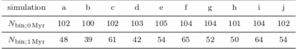
Table 2.The numbers of binaries in the separation range 62–620 au in the Plummer sphere cluster simulations at 0 Myr (first row) and at 1 Myr (second row). Not all 106 binaries are physically bound at the start of each simulation due to the high initial densities of the Plummer spheres.
simulation a b c d e f g h i j
Nbin;0 Myr 102 100 102 103 105 104 104 101 104 102
Nbin;1 Myr 48 39 61 42 54 65 52 50 64 54
3 RESULTS
Our initial binary population is formed with 106 binaries in the range 62 – 620 au, and this is the initial population foreverycluster. Clusters differ only in the random number seeds which set the system positions and velocities, not the system properties.
In this Section, we will first examine the differences in the numbers of intermediate binaries which are destroyed after 1 Myr, before turning our attention to the separation distributions and the mass ratio distributions of these bina-ries.
3.1 Binary fraction
In Table 1 we present the initial (0 Myr) and final (1 Myr) numbers of binaries in the separation range 62–620 au in each of the ten fractal cluster simulations. Each cluster has 106 binaries in this range initially, but the final number of binaries varies significantly, with extrema of 62 and 87 bina-ries (simulations i and a, respectively). Thus between 42 per cent and 18 per cent of the initial population has been de-stroyed. Looking just at this range, we started with 212 stars in 106 systems (a binary fraction of unity4) and the extremes after 1 Myr are 212 stars in 150 systems (a binary fraction of 0.41) and 212 stars in 125 systems (a binary fraction of 0.70).
Turning to the Plummer sphere clusters, in Table 2 we show the initial (0 Myr) and final (1 Myr) numbers of bina-ries in the separation range 62–620 au for each of our ten simulated clusters. There is a slight variation in the initial number of binaries detected by our algorithm (and no clus-ter has its full compliment of 106 initial binaries identified), due to the high initial densities of the Plummer spheres.
In the two most extreme cases, 39 binaries remain in a cluster that contained 100 initially (simulation b), and 65 binaries remain in a cluster that contained 105 initially
4 We define the binary fraction, f
bin = S+BB, where B is the number of binaries (and higher order multiple systems), andSis the number of singles.
(simulation f). Thus between 71 per cent and 37 per cent of the initial population has been destroyed. In terms of the binary fraction, we started with 212 stars in 112 systems (a binary fraction of 0.89 – simulation b), and 212 stars in 108 systems (a binary fraction of 0.96 – simulation f). After 1 Myr the binary fractions in these clusters are 0.23 and 0.44, respectively.
Thetotal binary fraction in the cluster of course also depends on the numbers of systems with separations outside of this range that have been destroyed.
More binaries are destroyed in the Plummer sphere clus-ters than the fractal clusclus-ters. The reason for this is that we produce an intermediate binary (say of separation 500 au) and place it at random within the simulation. If the binary is placed in a low-density region where the typical separation between stars is, say, 3000 au, then it is clearly identified as a binary system. However, if a 500 au binary is placed in a dense region with a typical inter-star separation of, say, 800 au, then it is no longer a ‘binary’. The handful of the 106 intermediate separation systems placed near the centre of a Plummer sphere are therefore ‘destroyed’ at time zero.
The localised substructure in the fractal clusters is not as dense as the central regions of the Plummer spheres, and so all binaries that ‘form’ in the fractals remain physically bound. The maxiumum densities in the fractal clusters are around 1000 – 2000 M⊙pc−3, whilst the central densities of the Plummer spheres are around 6−7×10⁴M⊙pc−3. There-fore, as the simulation progresses there will be significantly more and closer encounters in the centres of the Plummer spheres, which process the intermediate binaries more than in fractal clusters. We noted above that after 1 Myr the 106 intermediate binaries in the fractal clusters had been reduced to between 62 and 87 systems. In the much denser Plummer spheres the final numbers of systems are between 39 and 65 – a far more destructive environment.
[image:5.612.143.445.235.285.2](a) (b) (c)
(d) (e) (f)
(g) (h) (i)
[image:6.612.42.536.76.719.2](j) (k) AVERAGE
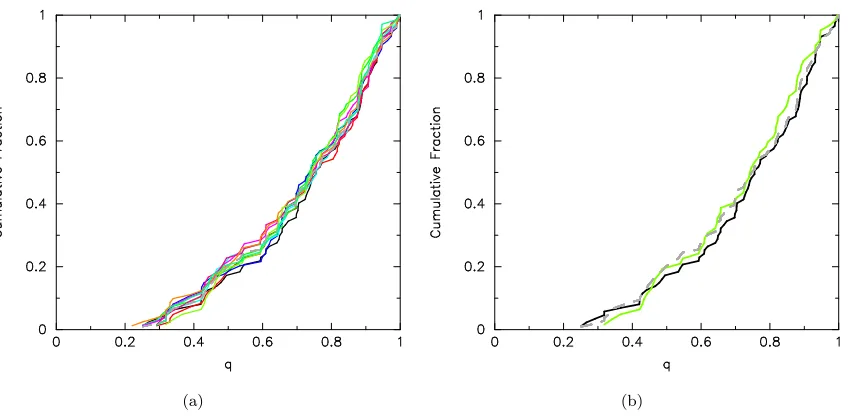
(a) (b)
Figure 2.The cumulative separation distribution of binaries in the separation range 62 – 620 au in (a) 10 different fractal clusters, and (b) the two extrema, after 1 Myr. The initial binary population is shown by the thick dashed grey line in both panels and is identical for each cluster.
3.2 Separation distribution
As well as changing the binary fraction in the intermediate 62 – 620 au range, the distribution of separations can also be changed significantly.
In Fig. 1 we show the individual separation distributions in the range 62 – 620 au for each fractal cluster, binned in the same way as the data in Reipurth et al. (2007). The initial separation distribution, which is identical in each simulation, is shown by the open histogram, and the separation distri-bution after 1 Myr is shown by the shaded histogram. For comparision, the data from Reipurth et al. (2007) is shown by the green crosses, and the log-normal fits to the field sep-aration distributions for G- and M-dwarfs are shown by the solid red and dashed blue lines, respectively. The average of all 10 simulations, with 1–σuncertainties, is shown in panel (k).
As noted in Parker et al. (2011), averaging together the 10 realisations of clusters with a fractal morphology and sub-virial velocities reproduces the observed ONC binary distri-bution reasonably well (see also King et al. 2012). However, from inspection of Fig. 1 we see that the same initial popula-tion can evolve to very different distribupopula-tions over the course of 1 Myr. Clearly, the initial population of 106 intermediate binaries is processed differently in each cluster.
In Fig. 2 we show the cumulative distributions of the in-termediate binary separations along with the initial separa-tion distribusepara-tion (the thick dashed grey line in both panels). In Fig. 2(a) all ten fractal realisations are shown, in Fig. 2(b) we show the two most different cumulative distributions.
In Fig. 3 we plot the 45 possible KS-test comparisons between the cumulative separation distributions of the frac-tal clusters. We reject the null hypothesis of there being no difference between two separation distributions if the KS p-value is less than 0.05.
The two most different separation distributions are from the distributions shown in panels (c) and (h) of Fig. 1. Note that these two simulations are not the same two simulations
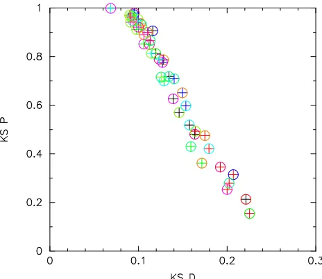
Figure 3.The distribution of values for KS tests between all pairs of the fractal cluster simulations on the cumulative separation distributions (colours correspond to those in Fig. 2). We show the KS p-value against the KSDstatistic.
that produce the largest difference in binary fraction (which were those in panels (a) and (i)).
The largest difference between the two extreme distri-butions isD= 0.26; for thisDa KS test gives the p–value P= 0.01. This is a very significant difference and one would draw the (correct) conclusion that these two distributions are different. However, it is not theinitialdistributions that were different (they were identical), rather it is the dynam-ical processing of the systems that was very different.
[image:7.612.307.544.356.555.2](a) (b)
Figure 4.The cumulative separation distribution of binaries in the separation range 62 – 620 au in (a) 10 different Plummer-sphere clusters, and (b) the two extrema, after 1 Myr. In panel (a) the thick dashed grey lines show the initial distributions which are slightly different for each cluster (see text), the differences are so small that in panel (b) we only plot the primordial distribution for the righthand cluster for clarity.
Figure 5.The distribution of values for KS tests between all pairs of the Plummer-sphere cluster simulations on the cumulative sep-aration distributions (colours correspond to those in Fig. 4). We show the KS p-value against the KSDstatistic.
each other (for the separation distribution, not necessarily, as we have seen, for binary fractions) shows that this simu-lation is just an outlier. However, the problem is that in just ten simulations we have produced a significant outlier, and there is no way of telling if a single observed distribution for a cluster is such an outlier.
Examination of Fig. 2(b) shows that one extreme (the lower orange line) remains very close to the initial separation distribution (the thick dashed grey line). This distribution is from panel (h) of Fig. 1 and it can be seen that it has lost roughly the same fraction of binaries from each bin so
retaining the shape of the initial distribution. The upper extreme (the green line) shows a very different separation distribution to the initial distribution, as can also be seen in panel (c) of Fig. 1 this cluster has mainly lost wider binaries (>200 au).
Generally speaking (and visible in Figs. 1 and 2), wider binaries are more susceptable to disruption as they are more weakly bound. A key result however is that because binary destruction is stochastic, the probability of destruction of an intermediatesystem depends more on if a system has had a close encounter or not than on the binding energy of the system (see Hills 1975; Heggie 1975).
One could hypothesise that the very different and stochastic dynamical histories of different fractals (see Allison et al. 2010) might be responsible for the very large differences in the resulting populations. To test this in Fig. 4 we plot the cumulative distributions of separations in our ten Plummer spheres for all ten realisations (panel (a)) and the two extremes (panel (b)) after 1 Myr along with the initial distribution (the thick dashed grey lines). Note that the initial distributions for each Plummer sphere are very slightly different, this is because some intermediate systems are in such a place that they are not identified as binaries even at time zero. Different realisations of Plummer spheres are almost impossible to distinguish, and their dynamical histories will be very similar. The only differences should be in the chance of a particular system having (a) destructive encounter(s) or not.
[image:8.612.45.277.366.567.2]are also significantly affected, and care must be taken not to take a marginal result for the KS test in separation distri-bution together with different binary fractions to make us suspect a real difference between clusters.
This may indicate that the differences in the final sep-aration distributions are due to the stochastic nature of the substructured fractals. However, as young, unevolved clus-ters appear to be substructured (Cartwright & Whitworth 2004; S´anchez & Alfaro 2009), and this substructure can dis-rupt binaries (Parker et al. 2011; King et al. 2012), then we must recognise that this stochasticity could affect our inter-pretation of observations of real clusters.
3.3 Mass ratio distribution
We have seen that the numbers and separation distribu-tions of intermediate binaries can be significantly altered in a highly stochastic way by encounters. We now turn our attention to the mass ratio distribution: is this also signif-icantly altered, or does it retain an imprint of the initial distribution? Note that the initial mass ratio distribution for our binary population is flat5.
In Figs. 6 and 7 we show the cumulative distributions of mass ratios in the intermediate 62 – 620 au range after 1 Myr of the fractal clusters (Fig. 6) and the Plummer spheres (Fig. 7). In both Figs. panel (a) shows all ten realisations, and panel (b) shows the two most extreme distributions. The initial mass ratio distributions are shown by the thick dashed grey lines (for the same reasons as in the separation disributions each Plummer sphere has aslightlydifferent ini-tial distribution).
Interestingly in the fractal clusters, the spread in the mass ratio distributions is rather low (Fig. 6), and even the two extremes look very similar (panel (b)). A KS test on these distributions fails to distinguish them.
However, in the Plummer spheres where processing has been much more extreme we see that the difference between the two extremes is greater than in the fractal clusters, but still not enough to be significantly different in a KS test.
Finally, we note that both the fractals and Plummer spheres with the two extremes in the final mass ratio distri-bution are not the same clusters with the extremes in the separation distribution.
Whether an encounter is destructive depends on the distance of that encounter and the binding energy of the bi-nary: a closer binary requires a closer encounter to destroy it. Binding energy also depends on the mass ratio, but these results suggest that the most important factor is the distance of the encounter (which depends on density but is stochastic with regards to the mass ratio of the system). In the case of the Plummer sphere clusters (Fig. 7(b)) both clusters have moreq <0.4 systems after processing than before (inspec-tion of Fig. 7(a) shows that this is not always the case). One extreme has stayed fairly close to the initial mass ratio distribution (the upper extreme), whilst the lower extreme
5 The cumulative initial mass ratio distributions in Figs. 6 and 7
are not straight lines despite being drawn from a flat mass ratio distribution. This is due to limiting the lower mass of companions to be>0.1 M⊙ meaning that M-dwarfs in particular do not fill the entire range of possible mass ratios. See Section 2.
has evolved to have far more very high mass ratio systems (q >0.9).
4 DISCUSSION
From the results presented in Section 3 we can see that stochasticity in the destruction of intermediate binaries can have a number of important consequences.
As would be expected, intermediate binary destruction depends on density. Dense environments are far more effec-tive at destroying intermediate binaries. Indeed, the defini-tion of what is a hard, soft, or intermediate binary depends on density – a hard binary in a very low-density environment could be an intermediate binary in another environment.
However, the range of (visual) binary separations in clusters normally probed by observations of 10s – 100s au covers the intermediate binary regime in the range of densi-ties found those clusters of 10−105 stars pc3 (see King et al. 2012). Therefore,we almost always observe intermediate binaries in star forming regions.
As would be expected, we find that the number of bina-ries processed depends on the density. But this processing is always stochastic with 18 – 42 per cent of intermediate bi-naries processed in the relatively low-density fractals, to 37 – 71 per cent in the higher-density Plummer spheres. There-fore,the number of intermediate binaries that are destroyed depends on density, but with a stochastic factor of around 2 in the number destroyed.
A key result is illustrated in Figs. 2 and 4 thatwhatever the density, the initial intermediate separation distribution can be significantly altered. Wider intermediate binaries are generally destroyed in preference to closer intermediates, but this is not a strong relationship. For an initially substruc-tured cluster, differences in processing can easily be extreme enough to show very strong statistical differences with e.g. a KS test. We emphasize here that only two different pairs of simulations resulted in significantly different separation distributions. However, we have no way of telling whether the clusters we observe in reality are themselves stochastic outliers.
Interestingly, as shown in Figs. 6 and 7 the change in the initial mass ratio distributions are not as strong as in the separation distributions. It seems thatintermediate bi-nary destruction does not care about the system mass ratio. That intermediate binary destruction is insensitive to mass ratio means that the processed mass ratio distributions are statistically the same as the initial mass ratio distribution. Therefore,in clusters with low levels of intermediate binary destruction, the mass ratio distribution should reflect the ini-tial mass ratio distribution. However, one has to know that there has been little processing to use this result.
These results have interesting implications for the inter-pretation of both observations and numerical simulations.
Clearly, when we observe a cluster we are observing a single realisation of its initial binary population and the pro-cessing of that population. When we compare two clusters we compare two different realisations and as we have seen, any two realisations may be very different, even if their ini-tial conditions were the same.
(a) (b)
Figure 6.The cumulative mass ratio distribution of binaries in the separation range 62 – 620 au in (a) 10 different fractal clusters, and (b) the two extrema, after 1 Myr. The initial distribution is shown by the thick dashed grey line in both panels.
(a) (b)
Figure 7.The cumulative mass ratio distribution of binaries in the separation range 62 – 620 au in (a) 10 different Plummer-sphere clusters, and (b) the two extrema, after 1 Myr. The initial distributions are shown by the thick dashed grey line in panel (a), but in panel (b) the initial distribution for the righthand cluster only is shown for clarity.
to note that processing occurs very quickly and so it is not the current density that is important, but the maximum density reached at some point in the past that determines how effective binary processing is (see also Goodwin 2010; Parker et al. 2009, 2011).
The problem we face when attempting to compare two intermediate binary populations and determine if they come from the same initial populations is therefore twofold. Firstly, we need to have information about the past state of the cluster to determine what level of processing we might expect on average. Secondly, we have to account for the stochasticity in intermediate binary destruction.
Let us take two ONC-like clusters as an example. We
started with 106 binaries in the observed 62–620 au range. (Actually, randomly sampling from the same underlying dis-tribution would give a range of 90 – 110 binaries initially in that range). We then find that 37 – 71 per cent of these can be destroyed in a dense cluster. Therefore in numbers of binaries alone, statistically the same initial population could result in between 39 and 65 binaries remaining in that range – a difference of over a factor of two from random chance alone. And this is before we consider the possibility that these two populations have also evolved to statistically different separation and mass ratio distributions.
[image:10.612.61.487.349.554.2]sig-inificant differences in the numbers of binaries, and the sep-arations and mass ratios of these binaries, then we might reasonably conclude that we were looking at two different initial populations and therefore a difference in how the stars were formed. However, as we have seen, that is sadly not the case.
Great care must also be taken when comparing simula-tions with observasimula-tions. It is standard procedure to average together the outcome of, say, ten simulations and compare the separation distribution (with standard deviation) to the observed one (e.g. Kroupa et al. 1999; Parker et al. 2009, 2011; King et al. 2012). However, the observed distribution may in fact be an outlier and a failure to fit the observed distribution might not mean that the model is ‘wrong’, con-versely, a good fit to the observed distribution does not mean the model is ‘right’ (correctly fitting an outlier would be wor-rying unless one’s simulation was also an outlier in the same way). Ensembles of simulations are crucial to at least deter-mine a reasonable tolerance for the model, however nothing will ever be able to determine if the observed realisation is an outlier or not.
In future papers we will examine the observed binary separation distributions in clusters from King et al. (2012) in light of these results, we will also examine what separation ranges are of use in distinguishing differences or otherwise in the star formation in different regions.
5 CONCLUSIONS
We have conducted N-body simulations of ONC-like clus-ters containing 1500 stars (750 primordial binary systems) in which we have kept the initial binary population constant, but varied the positions and velocities of the systems within ten realisations of the same cluster. We have studied two dif-ferent cluster morpholgies; a fractal cluster undergoing cool collapse (e.g. Allison et al. 2010) and a Plummer sphere in virial equilibrium (e.g. Parker et al. 2009). We have com-pared the intermediate separation distribution (62 – 620 au) in these clusters to examine the importance of stochasticity in intermediate binary destruction.
We conclude the following:
(i) The numbers of intermediate systems destroyed in clus-ters can vary by a factor of two.
(ii) The separation distributions of intermediate systems in substuctured clusters can be altered such that they are sta-tistically significantly different after just 1 Myr.
(iii) The mass ratio distributions change less than the sepa-ration distributions, especially in low-density environments. The results imply that the intermediate binary separa-tion distribusepara-tion, which is the range most often observed in young clusters, should be treated with caution when used to interpret the dynamical history of a star cluster. Even with a knowledge of the initial conditions and probable dynamical history of a cluster, stochasticity in intermediate binary de-struction can very significantly alter the initial population. Whilst most clusters evolve in a ‘typical’ way, statistically significant outliers are not uncommon and we have no way of knowing if a single observed cluster is unusual because of differences in the initial conditions, or through a slightly unusual dynamical evolution.
ACKNOWLEDGEMENTS
We thank the anonymous referee for a prompt and helpful review. The simulations in this work were performed on the BRUTUScomputing cluster at ETH Z¨urich.
REFERENCES
Aarseth S. J., H´enon M., Wielen R., 1974, A&A, 37, 183 Allison R. J., Goodwin S. P., 2011, MNRAS, 415, 1967 Allison R. J., Goodwin S. P., Parker R. J., de Grijs R.,
Portegies Zwart S. F., Kouwenhoven M. B. N., 2009, ApJ, 700, L99
Allison R. J., Goodwin S. P., Parker R. J., Portegies Zwart S. F., de Grijs R., 2010, MNRAS, 407, 1098
Bastian N., Covey K. R., Meyer M. R., 2010, ARA&A, 48, 339
Binney J., Tremaine S., 1987, Galactic Dynamics. Prince-ton, NJ, Princeton University Press, 1987, 747 p. Cartwright A., Whitworth A. P., 2004, MNRAS, 348, 589 Duquennoy A., Mayor M., 1991, A&A, 248, 485
Fischer D. A., Marcy G. W., 1992, ApJ, 396, 178
Goodwin S. P., 2010, Royal Society of London Philosophi-cal Transactions Series A, 368, 851
Goodwin S. P., Kroupa P., 2005, A&A, 439, 565 Goodwin S. P., Whitworth A. P., 2004, A&A, 413, 929 Heggie D. C., 1975, MNRAS, 173, 729
Hillenbrand L. A., Hartmann L. W., 1998, ApJ, 492, 540 Hills J. G., 1975, AJ, 80, 809
Kaczmarek T., Olczak C., Pfalzner S., 2011, A&A, 528, 144 King R. R., Parker R. J., Patience J., Goodwin S. P., 2012,
MNRAS, 421, 2025
Kroupa P., 1995a, MNRAS, 277, 1491 Kroupa P., 1995b, MNRAS, 277, 1507 Kroupa P., 2002, Science, 295, 82
Kroupa P., 2008, in Aarseth S. J., Tout C. A., Mardling R. A., eds, Lecture Notes in Physics, Berlin Springer Ver-lag Vol. 760 of Lecture Notes in Physics, Berlin Springer Verlag, Initial Conditions for Star Clusters. pp 181–259 Kroupa P., Petr M. G., McCaughrean M. J., 1999, New
Astronomy, 4, 495
Mayor M., Duquennoy A., Halbwachs L., Mermilliod J.-C., 1992, in McAlister H. A., Hartkopf W. I., eds, IAU Colloq. 135: Complementary Approaches to Double and Multiple Star Research Vol. 32 of ASP Conference Series, CORAVEL Surveys to Study Binaries of Different Masses and Ages. IAU, pp 73–81
Moeckel N., Clarke C. J., 2011, MNRAS, 415, 1179 Parker R. J., Goodwin S. P., Allison R. J., 2011, MNRAS,
418, 2565
Parker R. J., Goodwin S. P., Kroupa P., Kouwenhoven M. B. N., 2009, MNRAS, 397, 1577
Patience J., Ghez A. M., Reid I. N., Matthews K., 2002, AJ, 123, 1570
Plummer H. C., 1911, MNRAS, 71, 460
Portegies Zwart S. F., McMillan S. L. W., Hut P., Makino J., 2001, MNRAS, 321, 199
Portegies Zwart S. F., Makino J., McMillan S. L. W., Hut P., 1999, A&A, 348, 117
Reggiani M. M., Meyer M. R., 2011, ApJ, 738, 60
Reipurth B., Guimar˜aes M. M., Connelley M. S., Bally J., 2007, AJ, 134, 2272
S´anchez N., Alfaro E. J., 2009, ApJ, 696, 2086