This is a repository copy of Network Impacts of a Road Capacity Reduction: Empirical Analysis & Model Predictions.
White Rose Research Online URL for this paper: http://eprints.whiterose.ac.uk/84533/
Version: Accepted Version
Article:
Watling, DP, Milne, DS and Clark, SD (2012) Network Impacts of a Road Capacity
Reduction: Empirical Analysis & Model Predictions. Transportation Research Part A: Policy and Practice, 46 (1). 167 - 189 (23). ISSN 0965-8564
https://doi.org/10.1016/j.tra.2011.09.010
© 2012, Elsevier. Licensed under the Creative Commons Attribution-NonCommercial-NoDerivatives 4.0 International http://creativecommons.org/licenses/by-nc-nd/4.0/
[email protected] https://eprints.whiterose.ac.uk/ Reuse
Unless indicated otherwise, fulltext items are protected by copyright with all rights reserved. The copyright exception in section 29 of the Copyright, Designs and Patents Act 1988 allows the making of a single copy solely for the purpose of non-commercial research or private study within the limits of fair dealing. The publisher or other rights-holder may allow further reproduction and re-use of this version - refer to the White Rose Research Online record for this item. Where records identify the publisher as the copyright holder, users can verify any specific terms of use on the publisher’s website.
Takedown
If you consider content in White Rose Research Online to be in breach of UK law, please notify us by
NETWORK IMPACTS OF A ROAD CAPACITY REDUCTION:
EMPIRICAL ANALYSIS & MODEL PREDICTIONS
David Watling
1, David Milne
1& Stephen Clark
2Abstract – In spite of their widespread use in policy design and evaluation, relatively little evidence has
been reported on how well traffic equilibrium models predict real network impacts. Here we present what we believe to be the first paper that together analyses the explicit impacts on observed route choice of an actual network intervention and compares this with the before-and-after predictions of a network equilibrium model. The analysis is based on the findings of an empirical study of the travel time and route choice impacts of a road capacity reduction. Time-stamped, partial licence plates were recorded across a series of locations, over a period of days both with and without the capacity reduction, and the data were ‘matched’ between locations using special-purpose statistical methods. Hypothesis tests were used to identify statistically significant changes in travel times and route choice, between the periods of days with and without the capacity reduction. A traffic network equilibrium model was then independently applied to the same scenarios, and its predictions compared with the empirical findings. From a comparison of route choice patterns, a particularly influential spatial effect was revealed of the parameter specifying the relative values of distance and travel time assumed in the generalised cost equations. When this parameter was ‘fitted’ to the data without the capacity reduction, the network model broadly predicted the route choice impacts of the capacity reduction, but with other values it was seen to perform poorly. The paper concludes by discussing the wider practical and research implications of the study’s findings.
1. INTRODUCTION
It is well known that altering the localised characteristics of a road network, such as a planned change in road capacity, will tend to have both direct and indirect effects. The direct effects are imparted on the road itself, in terms of how it can deal with a given demand flow entering the link, with an impact on travel times to traverse the link at a given demand flow level. The indirect effects arise due to drivers changing their travel decisions, such as choice of route, in response to the altered travel times. There are many practical circumstances in which it is desirable to forecast these direct and indirect impacts in the context of a systematic change in road capacity.
For example, in the case of proposed road widening or junction improvements, there is typically a need to justify economically the required investment in terms of the benefits that will likely accrue. There are also several examples in which it is relevant to examine the impacts of road capacity reduction. For example, if one proposes to reallocate road space between alternative modes, such as increased bus and cycle lane provision or a pedestrianisation scheme, then typically a range of alternative designs exist which may differ in their ability to accommodate efficiently the new traffic and routing patterns. Through mathematical modelling, the alternative designs may be tested in a simulated environment and the most efficient selected for implementation. Even after a particular design is selected, mathematical models may be used to adjust signal timings to optimise the use of the transport system. Road capacity may also be affected periodically by maintenance to essential services (e.g. water, electricity) or the road itself, and often this can lead to restricted access over a period of days and weeks. In such cases, planning authorities may use modelling to devise suitable diversionary advice for drivers, and to plan any temporary changes to traffic signals or priorities. Berdica (2002) and Taylor et al (2006) suggest more of a pro-active approach, proposing that
1
Institute for Transport Studies, University of Leeds, Woodhouse Lane, Leeds LS2 9JT, UK.
2
models should be used to test networks for potential vulnerability, before any reduction materialises, identifying links which if reduced in capacity over an extended period3 would have a substantial impact on system performance.
There are therefore practical requirements for a suitable network model of travel time and route choice impacts of capacity changes. The dominant method that has emerged for this purpose over the last decades is clearly the network equilibrium approach, as proposed by Beckmann et al (1956) and developed in several directions since. The basis of using this approach is the proposition of
what are believed to be ‘rational’ models of behaviour and other system components (eg link performance functions), with site-specific data used to tailor such models to particular case studies. Cross-sectional forecasts of network performance at specific road capacity states may then be made, such that at the time of any ‘snapshot’ forecast, drivers’ route choices are in some kind of individually-optimum state. In this state, drivers cannot improve their route selection by a unilateral change of route, at the snapshot travel time levels.
The accepted practice is to ‘validate’ such models on a case-by-case basis, by ensuring that the modelwhen supplied with a particular set of parameters, input network data and input origin-destination demand datareproduces current measured mean link traffic flows and mean journey times, on a sample of links, to some degree of accuracy (see, for example, the practical guidelines in TMIP, 1997, and Highways Agency, 2002). This kind of aggregate level, cross-sectional validation to existing conditions persists across a range of network modelling paradigms, ranging from static and dynamic equilibrium (Florian & Nguyen, 1976; Leonard & Tough, 1979; Stephenson & Teply, 1984; Matzoros et al, 1987; Janson et al, 1986; Janson, 1991) to micro-simulation approaches (Laird et al, 1999; Ben-Akiva et al, 2000; Keenan, 2005).
While such an approach is plausible, it leaves many questions unanswered, and we would particularly highlight two:
1. The process of calibration and validation of a network equilibrium model may typically occur in a cycle. That is to say, having initially calibrated a model using the base data sources, if the subsequent validation reveals substantial discrepancies in some part of the network, it is then natural to adjust the model parameters (including perhaps even the OD matrix elements) until the model outputs better reflect the validation data4. In this process, then, we allow the adjustment of potentially a large number of network parameters and input data in order to replicate the validation data, yet these data themselves are highly aggregate, existing only at the link level. To be clear here, we are talking about a level of coarseness even greater than that in aggregate choice models, since we cannot even infer from link-level data the aggregate shares on alternative routes or OD movements. The question that arises is then: how many different combinations of parameters and input data values might lead to a similar link-level validation, and even if we knew the answer to this question, how might we choose between these alternative combinations? In practice, this issue is typically neglected, meaning that the
‘validation’ is a rather weak test of the model.
2. Since the data are cross-sectional in time (i.e. the aim is to reproduce current base conditions in equilibrium), then in spite of the large efforts required in data collection, no empirical evidence is routinely collected regarding the model’s main purpose, namely its ability to predict changes
3
Clearly, more sporadic and less predictable reductions in capacity may also occur, such as in the case of breakdowns and accidents, and environmental factors such as severe weather, floods or landslides (see, for example, Iida, 1999), but the responses to such cases are outside the scope of the present paper.
4
in behaviour and network performance under changes to the network/demand. This issue is
exacerbated by the aggregation concerns in point 1: the ‘ambiguity’ in choosing appropriate parameter values to satisfy the aggregate, link-level, base validation strengthens the need to independently verify that, with the selected parameter values, the model responds reliably to changes. Although such problemsof fitting equilibrium models to cross-sectional datahave long been recognised by practitioners and academics (see, e.g., Goodwin, 1998), the approach described above remains the state-of-practice.
Having identified these two problems, how might we go about addressing them? One approach to the first problem would be to return to the underlying formulation of the network model, and instead require a model definition that permits analysis by statistical inference techniques (see, for example, Nakayama et al, 2009). In this way, we may potentially exploit more information in the variability of the link-level data, with well-defined notions (such as maximum likelihood) allowing a systematic basis for selection between alternative parameter value combinations.
However, this approach is still using rather limited data and it is natural not just to question the model but also the data that we use to calibrate and validate it. Yet this is not altogether straightforward to resolve. As Mahmassani & Jou (2000) remarked: ‘A major difficulty … is obtaining observations of actual trip-maker behaviour, at the desired level of richness,
simultaneously with measurements of prevailing conditions’. For this reason, several authors have turned to simulated gaming environments and/or stated preference techniques to elicit information on drivers’ route choice behaviour (e.g. Mahmassani & Herman, 1990; Iida et al, 1992; Khattak et al, 1993; Vaughn et al, 1995; Wardman et al, 1997; Jou, 2001; Chen et al, 2001). This provides potentially rich information for calibrating complex behavioural models, but has the obvious limitation that it is based on imagined rather than real route choice situations.
Aside from its common focus on hypothetical decision situations, this latter body of work also signifies a subtle change of emphasis in the treatment of the overall network calibration problem. Rather than viewing the network equilibrium calibration process as a whole, the focus is on particular components of the model; in the cases above, the focus is on that component concerned with how drivers make route decisions. If we are prepared to make such a component-wise analysis, then certainly there exists abundant empirical evidence in the literature, with a history across a
number of decades of research into issues such as the factors affecting drivers’ route choice (e.g.
Wachs, 1967; Huchingson et al, 1977; Abu-Eiseh & Mannering, 1987; Antonisse et al, 1989; Bekhor et al, 2002; Liu et al, 2004), the nature of travel time variability (e.g. Smeed & Jeffcoate, 1971; Montgomery & May, 1987; May et al, 1989; McLeod et al, 1993), and the factors affecting traffic flow variability (Bonsall et al, 1984; Huff & Hanson, 1986; Ribeiro, 1994; Rakha & Van Aerde, 1995; Fox et al, 1998).
While these works provide useful evidence for the network equilibrium calibration problem, they do not provide a framework in which we can judge the overall ‘fit’ of a particular network model in the light of uncertainty, ambient variation and systematic changes in network attributes, be they related to the OD demand, the route choice process, travel times or the network data. Moreover, such data does nothing to address the second point made above, namely the question of how to validate the model forecasts under systematic changes to its inputs. The studies of Mannering et al (1994) and Emmerink et al (1996) are distinctive in this context in that they address some of the empirical concerns expressed in the context of travel information impacts, but their work stops at the stage of the empirical analysis, without a link being made to network prediction models. The focus of the present paper therefore is both to present the findings of an empirical study and to link this empirical evidence to network forecasting models.
paper is their location-specific analysis of link flows at 24 locations; by computing the root mean square difference in flows between successive weeks, and comparing the trend for 2006 with that for 2007 (the latter with the bridge collapse), they observed an apparent transient impact of the bridge collapse. They also showed there was no statistically-significant evidence of a difference in the pattern of flows in the period September-November 2007 (a period starting six weeks after the bridge collapse), when compared with the corresponding period in 2006. They suggested that this
was indicative of the length of a ‘re-equilibration process’ in a conceptual sense, though did not explicitly compare their empirical findings with those of a network equilibrium model.
The structure of the remainder of the paper is as follows. In §2 we describe the process of selecting the real-life problem to analyse, together with the details and rationale behind the survey design. Following this, §3 describes the statistical techniques used to extract information on travel times and routing patterns from the survey data. Statistical inference is then considered in §4, with the aim of detecting statistically significant explanatory factors. In §5 comparisons are made between the observed network data and those predicted by a network equilibrium model. Finally, in §6 the conclusions of the study are highlighted, and recommendations made for both practice and future research.
2. EXPERIMENTAL DESIGN
The ultimate objective of the study was to compare actual data with the output of a traffic network equilibrium model, specifically in terms of how well the equilibrium model was able to correctly forecast the impact of a systematic change applied to the network. While a wealth of surveillance data on link flows and travel times is routinely collected by many local and national agencies, we did not believe that such data would be sufficiently informative for our purposes. The reason is that while such data can often be disaggregated down to small time step resolutions, the data remains aggregate in terms of what it informs about driver response, since it does not provide the opportunity to explicitly trace vehicles (even in aggregate form) across more than one location. This has the effect that observed differences in link flows might be attributed to many potential causes: it is especially difficult to separate out, say, ambient daily variation in the trip demand matrix from systematic changes in route choice, since both may give rise to similar impacts on observed link flow patterns across recorded sites. While methods do exist for reconstructing OD and network route patterns from observed link data (e.g. Yang et al, 1994), these are typically based on the premise of a valid network equilibrium model: in this case then, the data would not be able to give independent information on the validity of the network equilibrium approach.
For these reasons it was decided to design and implement a purpose-built survey. However, it would not be efficient to extensively monitor a network in order to wait for something to happen, and therefore we required advance notification of some planned intervention. For this reason we chose to study the impact of urban maintenance work affecting the roads, which UK local government authorities organise on an annual basis as part of their ‘Local Transport Plan’. The city council of York, a historic city in the north of England, agreed to inform us of their plans and to assist in the subsequent data collection exercise.
our own requirement greatly reduced the candidate set of studies to monitor. A further consideration in study selection was its timing in the year for scheduling before/after surveys so to avoid confounding effects of known significant ‘seasonal’ demand changes, e.g. the impact of the change between school semesters and holidays. A further consideration was York’s role as a major tourist attraction, which is also known to have a seasonal trend. However, the impact on car traffic is relatively small due to the strong promotion of public transport and restrictions on car travel and parking in the historic centre. We felt that we further mitigated such impacts by subsequently choosing to survey in the morning peak, at a time before most tourist attractions are open.
Aside from the question of which intervention to survey was the issue of what data to collect. Within the resources of the project, we considered several options. We rejected stated preference survey methods as, although they provide a link to personal/socio-economic drivers, we wanted to compare actual behaviour with a network model; if the stated preference data conflicted with the network model, it would not be clear which we should question most. For revealed preference data, options considered included (i) self-completion diaries (Mahmassani & Jou, 2000), (ii) automatic tracking through GPS (Jan et al, 2000; Quiroga et al, 2000; Taylor et al, 2000), and (iii) licence plate surveys (Schaefer, 1988). Regarding self-completion surveys, from our own interview experiments with self-completion questionnaires it was evident that travellers find it relatively difficult to recall and describe complex choice options such as a route through an urban network, giving the potential for significant errors to be introduced. The automatic tracking option was believed to be the most attractive in this respect, in its potential to accurately map a given
individual’s journey, but the negative side would be the potential sample size, as we would need to
purchase/hire and distribute the devices; even with a large budget, it is not straightforward to identify in advance the target users, nor to guarantee their cooperation.
Licence plate surveys, it was believed, offered the potential for compromise between sample size and data resolution: while we could not track routes to the same resolution as GPS, by judicious location of surveyors we had the opportunity to track vehicles across more than one location, thus providing route-like information. With time-stamped licence plates, the matched data would also provide journey time information. The negative side of this approach is the well-known potential for significant recording errors if large sample rates are required. Our aim was to avoid this by recording only partial licence plates, and employing statistical methods to remove the impact of
‘spurious matches’, i.e. where two different vehicles with the same partial licence plate occur at
different locations.
Moreover, extensive simulation experiments (Watling & Maher, 1992; Watling, 1994) had previously shown that these latter statistical methods were effective in recovering the underlying movements and travel times, even if only a relatively small part of the licence plate were recorded, in spite of giving a large potential for spurious matching. We believed that such an approach reduced the opportunity for recorder error to such a level to suggest that a 100% sample rate of vehicles passing may be feasible. This was tested in a pilot study conducted by the project team, with dictaphones used to record a 100% sample of time-stamped, partial licence plates. Independent, duplicate observers were employed at the same location to compare error rates; the same study was also conducted with full licence plates. The study indicated that 100% surveys with dictaphones would be feasible in moderate traffic flow, but only if partial licence plate data were used in order to control observation errors; for higher flow rates or to obtain full number plate data, video surveys should be considered. Other important practical lessons learned from the pilot included the need for clarity in terms of vehicle types to survey (e.g. whether to include motor-cycles and taxis), and of the phonetic alphabet used by surveyors to avoid transcription ambiguities.
likely affected movements and alternative routes (using local knowledge of York CC, together with an existing network model of the city), in order to determine the number and location of survey sites; feasible viewpoints, based on site visits; the timing of surveys, e.g. visibility issues in the dark, winter evening peak period; the peak duration from automatic traffic flow data; and specific survey days, in view of public/school holidays. Our budget led us to survey the majority of licence plate sites manually (partial plates by audiotape or, in low flows, pen and paper), with video surveys limited to a small number of high-flow sites. From this combination of techniques, 100% sampling rate was feasible at each site. Surveys took place in the morning peak due both to visibility considerations and to minimise conflicts with tourist/special event traffic. From automatic traffic count data it was decided to survey the period 7:45– as the main morning peak period. This design process led to the identification of two studies:
Lendal Bridge study (Figure 1). Lendal Bridge, a critical part of York’s inner ring road, was scheduled to be closed for maintenance from September 2000 for a duration of several weeks. To
avoid school holidays, the ‘before’ surveys were scheduled for June and early September. It was
decided to focus on investigating a significant southwest-to-northeast movement of traffic, the river providing a natural barrier which suggested surveying the six river crossing points (C, J, H, K, L, M in Fig 1). In total, thirteen locations were identified for survey, in an attempt to capture traffic on both sides of the river as well as a crossing.
Fishergate study (Figure 2). The partial closure (capacity reduction) of the street known as
Fishergate, again part of York’s inner ring road, was scheduled for July 2001 to allow repairs to a collapsed sewer. Survey locations were chosen in order to intercept clockwise movements around the inner ring road, this being the direction of the partial closure. A particular aim was to detect rerouting from Fulford Road (site E in Fig 2), the main radial affected, with F and K monitoring local diversion possibilities, and sites G, H, I, J to capture wider-area diversion.
In both studies, the plan was to survey the selected locations in the morning peak over a period of approximately twenty weekdays, covering the three periods before, during and after the intervention, with the days selected so as to avoid any known public holidays or special events.
In the Lendal Bridge study, while the ‘before’ surveys proceeded as planned, the bridge’s actual first day of closure on September 11th 2000 also marked the beginning of the UK fuel protests (BBC, 2000a; Lyons & Chaterjee, 2002). Traffic flows were considerably affected by the scarcity of fuel, with congestion extremely low in the first week of closure, to the extent that any changes could not be attributed to the bridge closure; neither had our design anticipated how to survey the impacts of the fuel shortages. We thus re-arranged our surveys to monitor more closely the planned re-opening of the bridge. Unfortunately these surveys were hampered by a second unanticipated event, namely the wettest autumn in the UK for 270 years and the highest level of flooding in York since records began (BBC, 2000b). The flooding closed much of the centre of York to road traffic, including our study area, as the roads were impassable, and therefore we abandoned the planned
In the Fishergate study, fortunately no extreme events occurred, allowing six ‘before’ and seven
‘during’ days to be surveyed, together with one additional day in the ‘during’ period when the works were temporarily removed. However, the works over-ran into the long summer school holidays, when it is well-known that there is a substantial seasonal effect of much lower flows and congestion levels. We did not believe it possible to meaningfully isolate the impact of the link fully re-opening while controlling for such an effect, and so our plans for ‘after re-opening’ surveys were abandoned.
3. ESTIMATION OF VEHICLE MOVEMENTS & TRAVEL TIMES
The data resulting from the surveys described in section 2 is in the form of (for each day and each study) a set of time-stamped, partial licence plates, observed at a number of locations across the network. Since the data include only partial plates, they cannot simply be matched across observation points to yield reliable estimates of vehicle movements, since there is ambiguity in whether the same partial plate observed at different locations was truly caused by the same vehicle. Indeed, since the observed system is ‘open’ in the sense that not all points of entry, exit,
generation and attraction are monitored the question is not just which of several potential matches
to accept, but also whether there is any match at all. That is to say, an apparent match between data at two observation points could be caused by two separate vehicles that passed no other observation point. The first stage of analysis therefore applied a series of specially-designed statistical techniques to reconstruct the vehicle movements and point-to-point travel time distributions from the observed data, allowing for all such ambiguities in the data. Although the detailed derivations of each method are not given here, since they may be found in the references provided, it is necessary to understand some of the characteristics of each method in order to interpret the results subsequently provided. Furthermore, since some of the basic techniques required modification relative to the published descriptions, then in order to explain these adaptations it is necessary to understand some of the theoretical basis.
3.1 Graphical method for estimating point-to-point travel time distributions
The preliminary technique applied to each data set was the graphical method described in Watling & Maher (1988). This method is derived for analysing partial registration plate data for
unidirectional movement between a pair of observation stations (referred to as an ‘origin’ and a ‘destination’). Thus in the data study here, it must be independently applied to given pairs of observation stations, without regard for the interdependencies between observation station pairs. On
the other hand, it makes no assumption that the system is ‘closed’; there may be vehicles that pass the origin that do not pass the destination, and vice versa.
superimposed upon a scatter of points over the whole region (which will primarily be the spurious matches). If we were to assume uniform arrival rates at the observation stations, then the spurious matches would be uniformly distributed over this plot; however, we shall avoid making such a restrictive assumption.
The method begins by making a coarse estimate of the total number of genuine matches across the whole of this plot. As part of this analysis we then assume knowledge of, for any randomly selected vehicle, the probabilities:
) ,..., 2 , 1 ( plate) on registrati partial of type the of is vehicle
Pr( kth k m
k
where 1 1
m kk .
The particular methods for estimating these probabilities in the case-study examples will be described in section 3.3. It is noted that in the original reference of this work, the simplifying assumption of equally-probable types was made throughout, i.e. 1 (k 1,2,...,m)
m
k , but the
analysis is readily generalised to the more general case considered here (see below).
Now, even if the streams of vehicles passing the origin and destination were entirely independent, we would still by chance get a number of possible matches, all of which would clearly be spurious. Given a total number of vehicle observations (disregarding the registration information) at the origin and destination respectively of n and 1 n , then there are 2 n1n2 pairs of observations that could match in this way ‘by chance’. But, under the assumption of independent traffic streams at the observation points, the probability of any randomly selected pair of observations having the same partial registration plate type, purely by chance, is:
m k k 1 2 t) independen streams if match, spuriousPr( .
Multiplying this probability by n1n2 gives the expected number of ‘chance’ matches (namely
m 1 k 2 k 2 1nn ) under the hypothesis of independent traffic streams. In any real study (where we hope
the independence assumption will fail, i.e. some vehicle pass both observation points), this figure
may then be used as an estimate of the ‘background level’ of spurious matches; subtracting this from the number of possible matches therefore gives an estimate of the number of genuine matches. However, this is a relatively crude method since we have treated the data en masse; since any point
on the scatter graph implies a ‘journey time’, this suggests that we should be able to deduce an
improved method that essentially exploits the plausibility of these implied journey times in different parts of the scatter plot (clearly negative values for the implied journey times could easily be ruled out for example, but our approach can go beyond this).
) (
) (
ˆ y y
F . Clearly this can be used to deduce an estimate of the genuine journey time
probability density, fˆ(y) ( y).
In simulation experiments, reported in Watling & Maher (1988), Fˆwas seen to be an ‘improper’ estimator, in that it is not guaranteed to be non-decreasing, and is not confined to the range [0,1].
On the other hand, there was seen to be a ‘trust region’, safely between the 20th
and 80th percentile, within which the method was seen to recover reliably the overall shape of the journey time densities specified to the simulation experiments.
3.2 Maximum likelihood estimation of no. of genuine matches and journey time parameters
While the graphical method is attractive as a first line of investigation, due to its limited assumptions, there have been found to be methods with much greater potential precision for point estimation, in particular for estimating quantities such as the number of genuine matches and moments of the journey time density (Watling, 1990), specifically the maximum likelihood method (Watling, 1994). This also has the advantage over the graphical method of being able to simultaneously analyse data from multiple entry and exit sites to the study area (we shall henceforth refer to these as ‘origins’ and ‘destinations’), rather than having to match origin-destination pairs independently or in some priority order. Clearly, by its name, the maximum likelihood method is a parametric technique, and its success depends on the validity of the distributional assumptions made. In extensive simulation trials, the method was seen to be robust to all assumptions (such as errors in the k probabilities) except for that of the assumed distributional form of the journey time density function of genuine matches (Watling, 1990).
The assumptions made are simply that: at each origin, traffic splits as a multinomial distribution
between the available destinations (including a ‘sink’ destination, representing vehicles observed at
an origin which do not travel to any of the observed destinations); the journey times between each origin-destination pair are Normally distributed; for each destination, before arriving at the destination, the combination of traffic from all origins is joined by traffic from a nuisance ‘source’ origin (representing vehicles observed at a destination that were not observed at any origin), which arrives according to a time-homogeneous Poisson process. The estimation task is then to estimate the parameters of this model, namely the multinomial split probabilities for each origin, the mean and variance of the Normal journey time distribution for each origin-destination movement, and the arrival rate of the nuisance source Poisson process for each destination.
Allowing for ambiguities in matching the data, a likelihood function may then be deduced, though this cannot be maximised analytically. A direct maximum likelihood technique thus involves numerically maximising a likelihood function with an enormous number of terms, relating to all the possible complete matchings of the observed data. Even with efficient gradient-based optimization algorithms, this was seen to limit the practicality of the method for large-scale data sets. Therefore, an alternative method was proposed, based on a general purpose statistical algorithm for maximum
likelihood estimation in the presence of ‘incomplete’ data. This method, known as the EM
algorithm, operates by alternately (i) (E-step) computing the expected complete data log-likelihood based on the current estimates of the parameters from step (ii); (ii) (M-step) forming estimates of the parameters by maximising the expected complete data log-likelihood from step (i). Each of these steps can be performed analytically, and are performed alternately until convergence.
by direct tracking of vehicle movements, with no matching ambiguity). It was found, however, that bias could arise in the parameter estimates in two circumstances, as described below.
Firstly, the presence of end effects may cause a bias most seriously in the multinomial split estimates, but also in the journey time parameters. Such effects arise due to the finite observation time intervals, meaning that a vehicle recorded within the observation period at an origin may travel to a destination but arrive outside the observation period there5. These are termed ‘end effects’ as they are most serious for vehicles observed towards the end of the origin observation periods. The impact is a systematic underestimation in the proportion of origin-vehicles that travel to each of the destinations. A secondary impact is a potential underestimation in the journey time mean and
variance, since the distribution is ‘right-censored’ by the destination period: vehicles with longer journey times are more likely to be missed. While a theoretical fix to the method is possible to overcome this problem (see Appendix, Watling, 1994), this is at a relatively high computational cost, as the resulting M-step of the EM algorithm is no longer analytically solvable, and numerical optimization must be used. The problem was seen instead to be more readily overcome at the experimental design stage, by adjusting the relative sizes of the observation periods: see the discussion of §2 and analysis of §4.1.
Secondly, if the assumed journey time distribution is a poor fit to the shape of the actual data, then the journey time parameter estimates may be poor, and this can have a knock-on effect to the estimates of the multinomial split probabilities (and hence the estimated number of genuine matches). This issue was addressed in the present study by first using the graphical method as an investigative technique to deduce an appropriate distributional form. This also required a (minor) generalisation of the original maximum likelihood matching method, which was based on an assumption of Normal journey times, to allow parameters of alternative distributional forms such as the lognormal to be estimated.
3.3 Estimation of registration plate type probabilities
An important input to all of the registration plate analysis methods described aboveas it affects the chance of a spurious matchis the estimate of the probabilities:
) ,..., 2 , 1 ( plate) on registrati partial
of type the
of is vehicle
Pr( kth k m
k .
A simple estimate can be made based on the assumption that all types are equally likely: we shall refer to this as the equi-probable estimate. In order to understand this issue better, we need to understand the system of assigning registration plates in the UK. In fact there have been several changes to the system of registering plates, meaning that at any one time one will observe vehicles corresponding to several systems. In particular the surveys were all conducted in a period where a now-defunct system of registration plate assignation was in operation. This meant that in the surveys to be analysed, the vast majority of partial registration plates were of the form ‘Xijk’, where the X can be one of 21 letters of the alphabet denoting the year of registration of the vehicle and the
‘ijk’ is a numerical code of up to three digits. Assuming all combinations of year letter and numerical code are theoretically possible to arise therefore gives 21000 combinations, i.e. possible
‘types’ in the terminology of the present paper. In fact, while this system described the vast
majority of possible ‘types’, there are also a small number of partial registration plates that do not, such as some very old vehicles following an older registration system, non-UK registration plates,
and some personalised number plates. It is difficult to estimate the true prevalence of such possibilities, so as an approximation we assumed that these in total amounted too a 1000 more possible types, giving 22000 possible types in total. Thus, the equi-probable estimate used was:
) 22000 ,..., 2 , 1 (
ˆ
22000
1
k k .
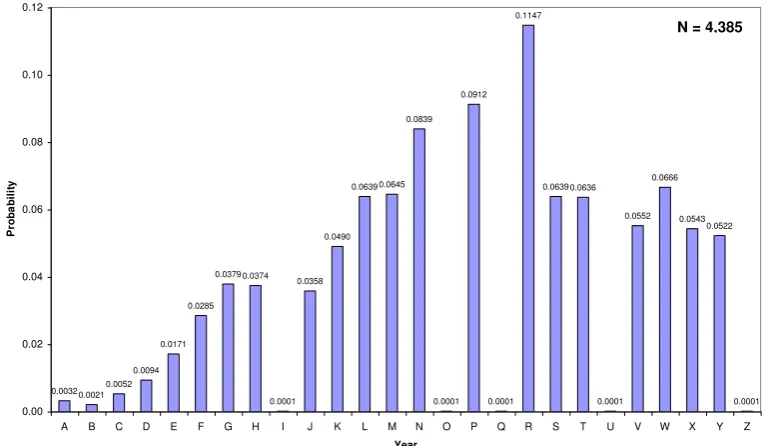
As an alternative to the equi-probable estimate, an empirical estimate was made from the available data for the Fishergate study. While in principle this would be possible for all year-letter and number combinations, a problem is that if we pool all data from all sites then there will be a natural bias (double-counting) toward vehicles passing more than one site; this is not a trivial issue since the whole purpose of these estimates is to distinguish the chance of a genuine or spurious match. If, on the other hand, we use only data from entry sites, then we will have many types observed only at exit sites for which we have no frequency information. The approach adopted, then, was to make an estimate of the year-letter frequencies, pooling all entry sites, while assuming the three-digit numerical components to be equally likely. The frequencies of year letter can be affected by several things, on the whole one would expect a decay going back in time as vehicles are scrapped, but on the other hand (local and global) economic factors will affect the rate at which new cars are purchased. The empirical distribution estimated from the data is given in Figure 3.
4. ANALYSIS OF STUDY DATA (OVER DAYS)
The methods described in section 3 were applied to each study site and to each day of data in turn. In the present section, we shall explore the combination of all such analyses over all study days.
4.1 Exploratory analysis of journey time distributions
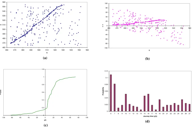
As a first step in the exploration of the data, the graphical method (described in §3.1) was applied to pairs of observation points for individual days in the survey period. As this method does not account for the interdependence in matching between anything more than two observation stations, the analysis is intended more for exploration, and to inform the subsequent parametric analysis. For illustration, we shall focus on the Fishergate study, and particularly on the movement most affected by the intervention, namely that from E to A. Figures 4(a)–4(d) give the results for this movement on the last day before the intervention (2nd July). Figure 4(a) shows the raw scatter plot of possible matches. Figure 4(b) presents the same information as in the scatter plot, but allows us to examine how the apparent journey times vary by observation time at E (i.e. the presence of any ‘dynamic
effects’). Figure 4(c) presents the estimated cumulative distribution function Fˆ corresponding to genuine matches. Finally, Figure 4(d) translates Fˆ into the form of an estimated journey time density function fˆ.
Consistently with the simulation experiments reported in Watling & Maher (1988), Figure 4(a) reflects (here for the real data) the characteristic clustering around the line ts, where is the mean journey time of genuine matches, and (s,t) is a pair of observation times at E and A respectively. Since the observation periods at both sites finish at the same time, some end effects must occur. From the upper right corner of the plot, it appears that this relates to vehicles passing E after time 550 (i.e. in the last ten minutes of the survey), since this is where the trend line is censored, but it would appear to affect relatively few vehicles. From Figure 4(b), since the trend line appears relatively flat, there appears to be no appreciable temporal effects within the survey period (such as a within-day change in journey time distribution). Figure 4(c) presents the estimated journey time cumulative distribution function, which appears to have a legitimate shape over the
density function over this trust region. Qualitatively similarly results were found for other movements over both days before the intervention and during the suspension day (figures not shown here due to space limitations): that is to say, a similar general shape of the density function, similar structure to the scatter plot, and the lack of any appreciable temporal effects.
A more interesting comparison is found by examining plots for this same movement (E to A) for the first two days during the intervention, namely 3rd and 4th July, respectively shown in Figures 5(a)– 5(d) and Figures 6(a)–6(d). Obviously, caution needs to be exercised in drawing more than indicative findings from this comparison, as it only involves a small number of days, but it does suggest important qualitative features to guide the further analysis. In particular, there are a number of striking contrasts between the plots for the intervention days and those without (not all shown here). Considering Figure 5(a), the dense trend line is more broken than in the ‘before’ case, the location of this line has shifted (indicating a location shift of the journey time distribution), and there is a much greater problem with end effects impacting on the last thirty minutes or more of the survey period at E. From Figure 5(b), there appears to be a build-up in journey times as the survey period progresses, as demonstrated by the slope of the dense trend line relative to the horizontal. Of particular relevance for the later parametric analysis, it is apparent from Figures 5(c)–5(d) that there has been a considerable change (relative to the ‘before’ situation) in the location, dispersion and shape of the journey time distribution, with a strong positive skew and much greater dispersion now evident. In Figures 6(a)–6(d), the evidence is similar, though with less apparent skewness in the distribution.
For reasons of space, we do not present here the equivalent graphs for other movements, but note that they did not demonstrate the same striking changes in the shape of the distribution as for the E to A movement. In particular, detailed attention was paid to two movements which, by their location, might also have been expected to be significantly affected, namely the E to K and G to A movements, with the resulting approximately symmetric journey time distributions for the two
‘during’ days resembling those for the ‘before’ and ‘suspension’ days.
Overall, the main suggestive evidence of this exploratory data analysis to take forward to the parametric analysis, were that a symmetric distribution of journey times appears to be a justifiable approximation for the vast majority of movements, but that for the journey E to A during periods of disruption there is evidence to suggest that a skewed distribution may on some days be more appropriate. Also, there is evidence of ‘end effects’, again especially for days during the intervention, which may need to be considered for their potential biasing effect on parameter estimates.
4.2 Parameter estimation for individual days & Between-day comparison tests
distribution function is effectively a coarse estimator of the number of genuine matches between a pair of points, and this may be divided by the total number of vehicles observed at an origin to obtain an initial estimate of the relevant multinomial split probability. This information may also be used to obtain an estimate of the number of nuisance source vehicles at each destination, and divided by the length of the observation period to get an estimate of the relevant Poisson rate. Finally, initial journey time estimates may clearly be made from the summary statistics of the density functions estimated by the graphical method. It is noted, however, that our tests here (not shown) confirmed earlier simulation results, that the EM algorithm final results were relatively insensitive to the choice of starting condition, so the precise manner of obtaining such initial estimates is not so important. Our discussion below will primarily focus on the Fishergate study, due to the better data quality in that case (as explained earlier), but we shall conclude by examining the Lendal Bridge study data to examine transferability of the qualitative findings to other sites.
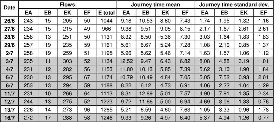
According to the exploratory data analysis of §4.1, Normal journey times were assumed in the maximum likelihood method in all cases, except for movement E to A during the capacity reduction, when a three-parameter log-normal was adopted. Table 1 contains selected results of this analysis for the Fishergate data in terms of the estimated number of genuine matches, and journey time mean and standard deviation, across all survey days. The matching is given for the most significant movements (in terms of their potential to be affected by the capacity change), namely E to A, E to B, E to K, E to F, G to A and G to B, where the survey locations are depicted on Figure 1. The columns of Table 1a are, working from the left, the date, the number of genuine matches for the four movements from E for that day, the total observed flow at E for that day (irrespective of whether it matched with any of the destination sites), the percentage of the flow at E which was matched with one of the destinations, and then similar information for the movements from point G.
For the purposes of an initial analysis it was decided to test between two groups of days: the five
‘before’ days, preceding July 3rd, and the six ‘during’ days where the capacity reduction was in operation, excluding the final two survey days (the temporary suspension day of July 13th and the day following it). The mean matched flow over the six during days (which can be calculated as 247.7) is substantially less than the mean over the five before days (297.6). A two-sample, unequal variance t-test for a reduction in the mean yields a one-sided p-value of p = 0.000872, and so this apparent reduction is highly significant.
This reduction in the EA flow could be due to a number of reasons; since the location of the capacity reduction means that this will be a major affected route, we investigate the potential reasons in some detail below:
1. Firstly, it might be that due to some external factors, the ‘during’ days were particularly ‘low
flow days’ generally. However, performing the same analysis as above on the mean total flow at E, then there is in fact an observed increase during the capacity reduction (from 1427.4 to 1495.8), though this is hardly significant (2-sided test, p = 0.092254)6. Thus, there is certainly no evidence that the total E flow is the cause of the reduction in the EA flow. It is noted that this
also apparently rules out ‘strategic’ re-routing, in the sense of there being no evidence of a decreased propensity to choose routes that pass through E as a result of the capacity reduction.
2. Secondly, it might be a ‘capacity’ effect, in the sense that a reduced throughput over a fixed time interval would be reflected in a decreased matched flow. In particular, it should be recalled that a substantial impact was observed when applying the graphical method in section 4.1 to the
‘during’ data for EA, resulting in significant problems with ‘end effects’. To explore the impact
of the end effects, the EM algorithm was re-applied to a reduced form of the data. This was
6
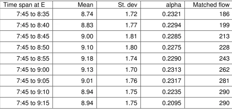
achieved by discarding origin data at point E that departed in the period after 8:55, that is to say discarding the last 20 minutes of the origin survey, but matching against the full survey periods at the other sites. The reason for choosing the time 8:55 is illustrated in Tables 2 and 3, whereby the truncation period at E has been altered over a range, and the impact on parameter estimates examined. For the 26th July, reductions below 9:10 begin to show an impact on the estimated
parameters, with the flow decreasing, as matches are “lost”. On the 3rd
July, however, a large reduction in the survey period is possible, down to less than 8:55, before the parameters begin to change.
Table 4 provides the counterpart to Table 1 for this truncated data set (i.e. with the ‘origin’ site truncated at 8:55). Clearly, as would be expected, the absolute number of matches are smaller than in the untruncated case. However, it can be verified that the truncation is successful in appreciably increasing the percentage of origin vehicles that are matched with some destination vehicle.
Repeating the test on the mean EA flow before and during the capacity reduction, the reduction from 250.0 to 237.3 gives a one-sided p-value of p = 0.033699. That is to say, the significance has been greatly reduced by the truncation, indicating that a major factor in the difference of the original (untruncated) EA matched flow was indeed a capacity effect. However, the difference is still highly significant, and so this is not the only explanatory factor.
3. Thirdly, there may have been a diversion away from EA, either because of advanced publicity of the road maintenance, en route diversion, or a ‘learning effect’. In particular we examine whether this could be the explanation for the remaining significance in the EA mean flow reduction, after the truncation described in point 2. above has been applied. This is achieved by examining, for each day, the proportion of the total vehicles observed at E that are EA-matched
journeys, and then testing the change in the mean proportion between the ‘before’ and ‘during’
days. This reveals a decrease in the fraction of drivers passing E that follow path EA, from 0.228 to 0.204, which (while it might appear small) is highly significant at a one-sided p = 0.000477. The reason for being able to detect significance with apparently such a small mean change is the remarkably small between-day variance in flow proportions for each of the two scenarios individually: the actual proportions being 0.233, 0.242, 0.228, 0.221, 0.216 before the capacity reduction; and 0.207, 0.200, 0.196, 0.213, 0.208, 0.200 during the capacity reduction. (In other words, the between-day variations in the EA flow are, taking either the ‘before’ or
‘during’ scenarios in isolation, most strongly explained by between-day variations in E, not by between-day variations in the fraction of E drivers selecting EA). It is noted, however, that one cannot discern any ‘learning’ effect, in the sense that the ‘during’ days are stable from the first day (perhaps an indicator of good advance warning of the works). In conclusion, it can be said that the capacity reduction certainly appears to have had a significant effect on the fraction of drivers passing E that select path EA.
Following a similar analysis for another of the major movements, EK, and making the truncation to remove end effects, a significant increase in the mean EK flow (from 233.0 to 285.8, one-sided test
for an increase: p = 0.002056) can be seen in comparing the ‘before’ and ‘during’ data.
Furthermore, when comparing the proportions of E flow following EK, there is again remarkably little between-day variation within either the ‘before’ or ‘during’ periods, but a highly significant increase in the mean proportion between the periods (from 0.212 to 0.246 at p = 0.00097). The analysis of flow proportions on EA and EK therefore suggests the data are consistent with a diversion away from EA to the alternative route EK, though we cannot attribute this with certainty.
As an illustration of the intervention’s impact on other movements (detailed figures not given due
the major movement GA, no significant mean change was detected at 5% significance in either the GA absolute flow, the G total flow, or the GA flow proportion. Examining the proportional flow GA of G over days, one obtains 0.406, 0.426, 0.419, 0.402, 0.413 before the intervention, and 0.443, 0.407, 0.376, 0.384, 0.398 for the days during the intervention. Again the proportions are quite stable within the before or during periods, except that the first day of the capacity reduction appears to stand out as slightly unusual: it has a substantially higher flow proportion than other days (and the lowest total flow at G). It might be postulated that this may be consistent with a learning effect, and if one could justify removing this day as unusual, then one does obtain a significant reduction in the mean GA proportions between the before and during cases (one sided test for a reduction, p = 0.022533).
Turning attention now to the journey time statistics, the first question is whether to base the analysis on Table 1 or Table 4. End effects have the potential to cause a bias in journey time statistics too, since they will tend to disproportionately affect longer journey times, leading to a potential underestimation in the journey time mean and standard deviation. However, examining the journey time results in Tables 1 and 4, there is no particularly clear evidence of this effect, and both sets of tables appear to show similar trends. Therefore, for the purposes of consistency with the graphical matching analysis (which was based on the full, untruncated data), and in order to maximise the sample size, we shall focus on Table 1, though the findings below would be qualitatively similar had we adopted the figures from Table 4.
We consider as an example again movement EA, and focus specifically on the first five survey days, before the capacity reduction. From Table 1, there is evidently quite substantial between-day variation in the mean journey time. Thus, even if we were to detect a change in the mean journey time between (say) the day before and day after the capacity reduction, this could not be confidently attributed to be an impact of the capacity reduction. However, treating each of the day-specific mean journey times as observations, we can compare the between-day mean of these means in the scenarios before and during the capacity reduction. In this comparison, the between-day mean shows an observed increase from 7.57 minutes to 10.28 minutes, whicheven in the light of the substantial between-day variation noted within each scenariois significant at p = 0.0118.
Having made the analyses and observations above based on the Fishergate study, we look to the Lendal Bridge data for the presence of corroborating or conflicting evidence with the qualitative findings above. Although the data are more limited (due to the problems described in section 2), they do appear to give some interesting corroborative insights. Looking to Figure 1, we particularly focus on the flows over the three bridges Lendal (site H), Ouse (site J) and Skeldergate (site C) which may be viewed as alternative river-crossing locations for flows from Blossom Street (site A, in the west) for traffic destined anywhere east of the river.
The results of the matching analysis from the EM algorithm are given in Table 5, where we specifically focus on the estimate of the number of genuine matches. As noted earlier (see §2), the
In particular, we may form 95% confidence intervals for the true mean flow from Blossom across each of the bridges, before the intervention, which yields confidence intervals (to the nearest integer) of [118, 156] for Lendal, [65,118] for Ouse and [89,205] for Skeldergate Bridges. These are notably rather wide confidence intervals, especially for Skeldergate, reflecting the considerable between-day variability observed, and in such a case it is perhaps not surprising that our single day
of ‘during’ data does not provide evidence of a significance change in the flow over this bridge (as
the single day of data, even neglecting the variability in the ‘during case’, is already within the 95%
confidence interval for the ‘before’ data). For the Ouse bridge the decision is more marginal, with
the ‘during’ observation on the boundary of the 95% confidence interval for the ‘before’ data, but had we allowed for the variability in the ‘during’ data then certainly here too we would have no evidence of a statistically significant change in flow. However, it is notable that one reason for this difficulty is the considerable day-to-day variability in the total flow from Blossom Street, as seen in Table 5.
This suggests adopting a similar strategy to that used in the Fishergate analysis, namely analysing the flow proportions over the bridges (i.e. as a proportion of the flow at site A). Forming 95% confidence intervals for the true mean proportions of flow at A choosing the different bridges, before the intervention, gives intervals of respectively [0.172, 0.200] for Lendal, [0.088, 0.160] for Ouse, and [0.153, 0.234] for Skeldergate. On the intervention day the proportion observed at Ouse was 0.213 and at Skeldergate 0.257, both outside the 95% confidence interval for the ‘before’ data. While we cannot conclude that this gives statistical significance without evidence of the day-to-day variability during the closure, it provides a qualitative indication of a potentially significant impact. This is not so surprising, given that we have closed one of three bridges and seen a change to the traffic choosing the two obvious alternative bridges; the main issue concerns the corroboration of the analysis of the earlier Fishergate data, where we were able to see considerably more chance of significant information arising from analysing flow proportions as opposed to absolute flows.
5. COMPARISON WITH NETWORK EQUILIBRIUM MODEL RESULTS
The final step of the study involved comparing the empirical data with the predictions of a traffic network equilibrium model. There are many reasons that make such a comparison less than straightforward, and particular issues that need to be borne in mind. Firstly, the question is what kind of network equilibrium in particular do we want to use, such as dynamic or static, deterministic (Wardrop) or stochastic user equilibrium, route choice based on mean travel times or on unreliability considerations, etc. In fact we decided to approach this problem from a practice-based perspective, and particularly what methods were commonly used in practice. This in fact opens up further model classes, which one does not often see considered in the academic literature, namely the models that have been developed for particular software packages that often lie somewhere between the distinctions seen in the academic literature.
In particular, we chose to use the so-called ‘simulation-assignment’ capabilities incorporated in the SATURN suite (Van Vliet, 1982), based on a representation of an asymmetric, static Wardrop equilibrium problem with junction interactions. This technique pays particular attention to the detail
of junction delays in urban networks, using an ‘exploded’ network definition in which each turn is represented by a link with its own flow-delay relationship. These flow-delay relationships are, however, not pre-specified, but are internally estimated during the assignment procedure, by fitting
curves to points generated by a ‘simulation’ model.The word ‘simulation’ is perhaps misleading: in
the traffic signal intersections. This flow propagation approach allows the method to overcome to some extent, albeit in a heuristic way, the problem of static traffic assignment models failing to impose capacity constraints on flows, with unserved demand held over on a link to be served in a subsequent modelled time period. The algorithm as a whole has the semblance of a diagonalisation algorithm: at one iteration of the diagonalisation, conditional on opposing/interacting flows as estimated from the previous iteration, separable flow-delay relationships are estimated for each link (turn) and a Frank-Wolfe algorithm is applied to find a Wardrop equilibrium route pattern conditional on those relationships. This route pattern is then fed into the subsequent iteration of the
diagonalisation, where a new ‘simulation’ is performed, new flow-delay relationships estimated, and a full Frank-Wolfe algorithm again applied. This heuristic method has no guarantee of convergence, though extensive use of it in practice indicates that it usually stabilises, except in highly congested networks.
We have given the details above for completeness, as they are not so readily found in the public domain, and because we felt that the method – while limited by the fact that it uses a static rather than dynamic user equilibrium – overcomes at least in a coarse way many of the concerns the reader might have with adopting a static approach. In fact our choice of method was also guided by the fact that a well-maintained, SATURN-based representation already existed for the City of York, and the fact that the project team had some considerable familiarity and experience with the software. Other software packages or other modelling methods could have been chosen, and in fact we shall not delve into the details of how well each of the elements of SATURN performs, as we wish to gain more general, qualitative findings about the model fit that are not specific to a particular software package. We believe that our qualitative findings below would hold good had other network equilibrium approaches been adopted, though we have not tested this claim.
Aside from the issue of which traffic assignment modelling representation/paradigm to choose, any comparison between a network equilibrium model and empirically-observed networks must also be made subject to several other considerations. Perhaps most significant among these is the issue of data quality: how good and up-to-date are the origin-destination matrix and the input network data? A quite different issue is the question of which numerical algorithm was used to implement the chosen paradigm: in our study we have used the Frank-Wolfe algorithm, for which we need to accept a likely larger convergence error than with several newer algorithms for solving Wardrop user equilibrium (e.g. Dial, 2006; Bar-Gera, 2010; Nie, 2010). While this in turn means a risk that part of the difference in any modelled comparison is attributable to such convergence error, we feel that the systematic nature of the results from the tests we report below provides evidence that, for the size of changes we have considered, the effects of changing the input parameters outweighs any convergence error (which is unlikely to lead to such systematic effects). In any case, we feel that such concerns about convergence error need to be weighed against those of the underlying model error, such as is caused by using of a single OD matrix and a single point equilibrium to approximate what is in fact a system with considerable real day-to-day variability.
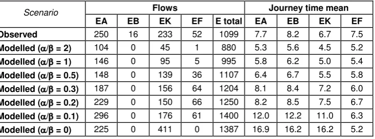
We performed the comparison of observed and modelled information in two distinct stages:
1. A comparison of mean flows and travel times between pairs of sites in the base situation, prior to the intervention, and with Fishergate modelled at full capacity, to ensure that the model provided a sufficiently faithful representation of observed route choice behaviour to use as a test-bed.
2. A comparison of mean flows and travel times between pairs of sites for the “during
intervention” days (those shaded in Table 1), with Fishergate now modelled at reduced capacity, to investigate the performance of the model in predicting changes in route choice behaviour.
It is worth emphasising the difference of this approach from ‘model validation’ as is commonly
applied in practice. The practical approach usually adopted is (i) to only validate the model in the base situation, i.e. there is no step 2, in the sense that the impacts of past interventions on a given network are not used to inform the modelling of future interventions; and (ii) to apply step 1 only at the level of aggregate link flows and average link travel times, not at the finer level of resolution used here of point-to-point flows and point-to-point travel times. Thus the validation tests applied here adopt a much higher standard, in asking the model to reproduce changes to some systematic input, and to reproduce those changes at a point-to-point rather than single-site level.
From the model, therefore, we need to extract information not just at the link level, but at a finer level of resolution. A potential drawback of this, especially for the Wardrop user equilibrium model, is that we may then be asking for information that is not uniquely defined by the model itself. It is well known that under the assumptions commonly adopted, user equilibrium link flows are unique but the route flows are typically non-unique; our level of interrogation will be between the level of link and route flow, and therefore also gives rise to potentially a non-unique model solution at this level. To be strict, then, what we compare from the model is the final solution obtained by the application of a Frank-Wolfe algorithm starting from initial free flow travel costs. Recently, Bar-Gera (2010) has investigated the prevalence of such non-unique outputs, and particularly the tendency for some equilibrium solution algorithms to stop at extreme solutions, favouring particular origin-destination movements. In the case of the Frank-Wolfe algorithm, however, Bar-Gera found much less evidence for such extreme behaviour, and we believe that this further supports our selection of the Frank-Wolfe algorithm and our decision to use model outputs at a higher level of resolution than link flows.