This is a repository copy of Linear Latent Force Models Using Gaussian Processes.
White Rose Research Online URL for this paper:
http://eprints.whiterose.ac.uk/120149/
Version: Submitted Version
Article:
Alvarez, M.A. orcid.org/0000-0002-8980-4472, Luengo, D. and Lawrence, N.D.
orcid.org/0000-0001-9258-1030 (2013) Linear Latent Force Models Using Gaussian
Processes. IEEE Transactions on Pattern Analysis and Machine Intelligence, 35 (11). pp.
2693-2705. ISSN 0162-8828
https://doi.org/10.1109/TPAMI.2013.86
[email protected] https://eprints.whiterose.ac.uk/ Reuse
Unless indicated otherwise, fulltext items are protected by copyright with all rights reserved. The copyright exception in section 29 of the Copyright, Designs and Patents Act 1988 allows the making of a single copy solely for the purpose of non-commercial research or private study within the limits of fair dealing. The publisher or other rights-holder may allow further reproduction and re-use of this version - refer to the White Rose Research Online record for this item. Where records identify the publisher as the copyright holder, users can verify any specific terms of use on the publisher’s website.
Takedown
If you consider content in White Rose Research Online to be in breach of UK law, please notify us by
Linear Latent Force Models using Gaussian Processes
Mauricio A. ´
Alvarez
†,‡, David Luengo
♯, Neil D. Lawrence
⋆,◦†School of Computer Science, University of Manchester, Manchester, UK M13 9PL. ‡Faculty of Engineering, Universidad Tecnol´ogica de Pereira, Colombia, 660003.
♯Dep. de la Teor´ıa de la Se˜nal y Comunicaciones, Universidad Carlos III de Madrid, 28911 Legan´es, Espa˜na.
⋆School of Computer Science, University of Sheffield, Sheffield, UK S1 4DP. ◦The Sheffield Institute for Translational Neuroscience, Sheffield, UK S10 2HQ.
Abstract
Purely data driven approaches for machine learning present difficulties when data is scarce relative to the complexity of the model or when the model is forced to extrapolate. On the other hand, purely mechanistic approaches need to identify and specify all the interactions in the problem at hand (which may not be feasible) and still leave the issue of how to parameterize the system. In this paper, we present a hybrid approach using Gaussian processes and differential equations to combine data driven modelling with a physical model of the system. We show how different, physically-inspired, kernel functions can be developed through sensible, simple, mechanistic assumptions about the underlying system. The versatility of our approach is illustrated with three case studies from motion capture, computational biology and geostatistics.
1
Introduction
Traditionally the main focus in machine learning has been model generation through adata driven paradigm. The usual ap-proach is to combine a data set with a (typically fairly flexible) class of models and, through judicious use of regularization, make predictions on previously unseen data. There are two key problems with purely data driven approaches. Firstly, if data is scarce relative to the complexity of the system we may be unable to make accurate predictions on test data. Secondly, if the model is forced to extrapolate,i.e.make predictions in a regime in which data has not yet been seen, performance can be poor.
Purelymechanistic models,i.e. models which are inspired by the underlying physical knowledge of the system, are com-mon in many domains such as chemistry, systems biology, climate modelling and geophysical sciences,etc.They normally make use of a fairly well characterized physical process that underpins the system, often represented with a set of differ-ential equations. The purely mechanistic approach leaves us with a different set of problems to those from the data driven approach. In particular, accurate description of a complex system through a mechanistic modelling paradigm may not be possible. Even if all the physical processes can be adequately described, the resulting model could become extremely com-plex. Identifying and specifying all the interactions might not be feasible, and we would still be faced with the problem of identifying the parameters of the system.
Despite these problems, physically well characterized models retain a major advantage over purely data driven models. A mechanistic model can enable accurate prediction even in regions where there is no available training data. For example, Pioneer space probes can enter different extra terrestrial orbits regardless of the availability of data for these orbits. Whilst data driven approaches do seem to avoid mechanistic assumptions about the data, typically the regularization which is applied encodes some kind of physical intuition, such as the smoothness of the interpolant. This does reflect a weak underlying belief about the mechanism that generated the data. In this sense the data driven approach can be seen asweakly mechanisticwhereas models based on more detailed mechanistic relationships could be seen asstrongly mechanistic. The observation that weak mechanistic assumptions underlie a data driven model inspires our approach. We suggest a
hybrid systemwhich involves a (typically overly simplistic) mechanistic model of the system. The key is to retain sufficient flexibility in our model to be able to fit the system even when our mechanistic assumptions are not rigorously fulfilled in practise. To illustrate the framework we will start by considering dynamical systems as latent variable models which incorporate ordinary differential equations. In this we follow the work of Lawrence et al. (2007) and Gao et al. (2008) who encoded a first order differential equation in a Gaussian process (GP). However, their aim was to construct an accurate model of transcriptional regulation, whereas ours is to make use of the mechanistic model to incorporate salient characteristics of the data (e.g.in a mechanical system inertia) without necessarily associating the components of our mechanistic model with actual physical components of the system. For example, for a human motion capture dataset we develop a mechanistic
model of motion capture that does not exactly replicate thephysicsof human movement, but nevertheless captures salient features of the movement. Having shown how linear dynamical systems can be incorporated in a GP, we finally show how partial differential equations can also be incorporated for modelling systems with multiple inputs.
The paper is organized as follows. In section 2 we motivate the latent force model using as an example a latent variable model. Section 3 employs a first order latent force model to describe how the general framework can be used in practise. We then proceed to show three case studies. In section 4 we use a latent force model based on a second order ordinary differential equation for characterizing motion capture datasets. Section 5 presents a latent force model for spatio-temporal domains applied to represent the development of Drosophila Melanogaster, and a latent force model inspired in a diffusion process to explain the behavior of pollutant metals in the Swiss Jura. Extensive related work is presented in section 6. Final conclusions are given in section 7.
2
From latent variables to latent functions
A key challenge in combining the mechanistic and data-driven approaches is how to incorporate the model flexibility associated with the data-driven approach within the mechanism. We choose to do this through latent variables, more precisely latent functions: unobserved functions from the system. To see how this is possible we first introduce some well known data driven models from a mechanistic latent-variable perspective.
Let us assume we wish to summarize a high dimensional data set with a reduced dimensional representation. For example, if our data consists of N points in aD dimensional space we might seek a linear relationship between the data, Y = [y1, . . . ,yD] ∈ RN×D withyd ∈ RN×1, and a reduced dimensional representation,U = [u1, . . . ,uQ] ∈ RN×Q with
uq ∈RN×1, whereQ < D. From a probabilistic perspective this involves an assumption that we can represent the data as
Y=UW⊤+E, (1)
whereE = [e1, . . . ,eD]is a matrix-variate Gaussian noise: each column,ed ∈ RN×1 (1 ≤ d ≤D), is a multi-variate Gaussian with zero mean and covarianceΣ, this is,ed∼ N(0,Σd). The usual approach, as undertaken in factor analysis and principal component analysis (PCA), to dealing with the unknown latent variables in this model is to integrate outU
under a Gaussian prior and optimize with respect toW∈RD×Q(although it turns out that for a non-linear variant of the
model it can be convenient to do this the other way around, see for example Lawrence (2005)). If the data has a temporal nature, then the Gaussian prior in the latent space could express a relationship between the rows ofU,utn =Γutn−1+η,
whereΓis a transformation matrix,ηis a Gaussian random noise andutnis then-th row ofU, which we associate with
timetn. This is known as theKalman filter/smoother. Normally the times,tn, are taken to be equally spaced, but more generally we can consider a joint distribution forp(U|t), for a vector of time inputst= [t1. . . tN]⊤, which has the form of a Gaussian process,
p(U|t) =
Q
Y
q=1
N uq|0,Kuq,uq
, (2)
where we have assumed zero mean and independence across theQdimensions of the latent space. The GP makes explicit the fact that the latent variables are functions, {uq(t)}Qq=1, and we have now described them with a process prior. The elements of the vectoruq = [uq(t1), . . . , uq(tN)]⊤, represents the values of the function for theq-th dimension at the times given byt. The matrixKuq,uq is the covariance function associated touq(t)computed at the times given int.
Such a GP can be readily implemented. Given the covariance functions for{uq(t)}Qq=1the implied covariance functions for {yd(t)}Dd=1 are straightforward to derive. In Teh et al. (2005) this is known as a semi-parametric latent factor model
(SLFM), although their main focus is not the temporal case. If the latent functionsuq(t)share the same covariance, but are sampled independently, this is known as the multi-task Gaussian process prediction model (MTGP) (Bonilla et al., 2008) with a similar model introduced in Osborne et al. (2008). Historically the Kalman filter approach has been preferred, perhaps because of its linear computational complexity in N. However, recent advances in sparse approximations have made the general GP framework practical (see Qui˜nonero-Candela and Rasmussen (2005) for a review).
So far the model described relies on the latent variables to provide the dynamic information. Our main contribution is to include a further dynamical system with amechanisticinspiration. We will make use of a mechanical analogy to introduce it. Consider the following physical interpretation of (1): the latent functions, uq(t), areQ forces and we observe the displacement ofDsprings,yd(t), to the forces. Then we can reinterpret (1) as the force balance equation,YB=US⊤+Ee. Here we have assumed that the forces are acting, for example, through levers, so that we have a matrix of sensitivities,
S ∈ RD×Q, and a diagonal matrix of spring constants, B ∈ RD×D, with elements {Bd}Dd=1. The original model is
recovered by setting W⊤ = S⊤B−1 and˜ed ∼ N 0,B⊤ΣdB
model this physical model underlies the Kalman filter, PCA, independent component analysis and the multioutput Gaussian process models we mentioned above. The use of latent variables means that despite this strong physical constraint these models are still powerful enough to be applied to a range of real world data sets. We will retain this flexibility by maintaining the latent variables at the heart of the system, but introduce a more realistic system by extending the underlying physical model. Let us assume that the springs are acting in parallel with dampers and that the system has mass, allowing us to write,
¨
YM+ ˙YC+YB=US+Eb, (3)
whereMandCare diagonal matrices of masses,{Md}Dd=1, and damping coefficients,{Cd}Dd=1, respectively,Y˙ is the first
derivative ofYwith respect to time (with entries{y˙d(tn)}ford= 1, . . . Dandn= 1, . . . , N),Y¨ is the second derivative ofYwith respect to time (with entries{y¨d(tn)}ford= 1, . . . Dandn= 1, . . . , N) andEb is once again a matrix-variate Gaussian noise. Equation (3) specifies a particular type of interaction between the outputsYand the set of latent functions
U, namely, that a weighted sum of the second derivative foryd(t),y¨d(t), the first derivative foryd(t),y˙d(t), andyd(t)is equal to the weighted sum of functions{uq(t)}Qq=1 plus a random noise. The second order mechanical system that this
model describes will exhibit several characteristics which are impossible to represent in the simpler latent variable model given by (1), such as inertia and resonance. This model is not only appropriate for data from mechanical systems. There are many analogous systems which can also be represented by second order differential equations, for example Resistor-Inductor-Capacitor circuits. A unifying characteristic for all these models is that the system is being forced by latent functions,{uq(t)}Qq=1. Hence, we refer to them aslatent force models(LFMs). This is our general framework: combine a physical system with a probabilistic prior over some latent variable.
One analogy for our model comes through puppetry. A marionette is a representation of a human (or animal) controlled by a limited number of inputs through strings (or rods) attached to the character. In a puppet show these inputs are the unobserved latent functions. Human motion is a high dimensional data set. A skilled puppeteer with a well designed puppet can create a realistic representation of human movement through judicious use of the strings
3
Latent Force Models in Practise
In the last section we provided a general description of the latent force model idea and commented how it compares to pre-vious models in the machine learning and statistics literature. In this section we specify the operational procedure to obtain the Gaussian process model associated to the outputs and different aspects involved in the inference process. First, we illus-trate the procedure using a first-order latent force model, for which we assume there are no masses associated to the outputs and the damper constants are equal to one. Then we specify the inference procedure, which involves maximization of the marginal likelihood for estimating hyperparameters. Next we generalize the operational procedure for latent force models of higher order and multidimensional inputs and finally we review some efficient approximations to reduce computational complexity.
3.1
First-order Latent Force Model
Assume a simplified latent force model, for which only the first derivative of the outputs is included. This is a particular case of equation (3), with masses equal to zero and damper constants equal to one. With these assumptions, equation (3) can be written as
˙
Y+YB=US+Eb. (4)
Individual elements in equation (4) follow
dyd(t)
dt +Bdyd(t) = Q
X
q=1
Sd,quq(t) + ˆed(t). (5)
Given the parameters{Bd}Dd=1and{Sd,q}D,Qd=1,q=1, the uncertainty in the outputs is given by the uncertainty coming from the set of functions {uq(t)}qQ=1 and the noiseeˆd(t). Strictly speaking, this equation belongs to a more general set of equations known asstochastic differential equations(SDE) that are usually solved using special techniques from stochastic calculus (Øksendal, 2003). The representation used in equation (5) is more common in physics, where it receives the name ofLangevin equations(Reichl, 1998). For the simpler equation (5), the solution is found using standard calculus techniques and is given by
yd(t) =yd(t0)e−Bdt+
Q
X
q=1
whereyd(t0)correspond to the value ofyd(t)fort =t0 (or the initial condition) andGdis a linear integral operator that follows
Gd[v](t) =fd(t, v(t)) =
Z t
0
e−Bd(t−τ)v(τ)dτ .
Our noise modelGd[ˆed](t)has a particular form depending on the linear operatorGd. For example, for the equation in (6) and assuming a white noise process prior fored(t), it can be shown that the processGd[ˆed](t)corresponds to the Ornstein-Uhlenbeck (OU) process (Reichl, 1998). In what follows, we will allow the noise model to be a more general process and we denote it bywd(t). Without loss of generality, we also assume that the initial conditions{yd(t0)}Dd=1 are zero, so that
we can write again equation (6) as
yd(t) = Q
X
q=1
Sd,qGd[uq](t) +wd(t). (7)
We assume that the latent functions{uq(t)}Qq=1are independent and each of them follows a Gaussian process prior, this is,
uq(t)∼ GP(0, kuq,uq(t, t′)).
1 Due to the linearity ofG
d,{yd(t)}Dd=1correspond to a Gaussian process with covariances
kyd,yd′(t, t′) = cov[yd(t), yd′(t′)]given by
cov[fd(t), fd′(t′)] + cov[wd(t), wd′(t′)]δd,d′,
whereδd,d′ corresponds to the Kronecker delta andcov[fd(t), fd′(t′)]is given by
Q
X
q=1
Sd,qSd′,qcov[fdq(t), f q d′(t′)],
where we usefdq(t)as a shorthand forfd(t, uq(t)). Furthermore, for the latent force model in equation (4), the covariance
cov[fdq(t), fdq′(t′)]is equal to
Z t
0
e−Bd(t−τ)
Z t′
0
e−Bd′(t′−τ′)k
uq,uq(τ, τ
′)dτ′dτ. (8)
Notice from the equation above that the covariance betweenfdq(t)andfdq′(t′)depends on the covariancekuq,uq(τ, τ′). We
alternatively denotecov[fd(t), fd′(t′)]askfd,f
d′(t, t′)andcov[f
q d(t), f
q
d′(t′)]askfdq,fdq′(t, t′). The form for the covariance kuq,uq(t, t′)is such that we can solve both integrals in equation (8) and find an analytical expression for the covariance
kfd,fd′(t, t′). In the rest of the paper, we assume the covariance for each latent forceuq(t)follows the squared-exponential (SE) form (Rasmussen and Williams, 2006)
kuq,uq(t, t′) = exp
−(t−t′)
2
ℓ2
q
, (9)
whereℓqis known as the length-scale. We can compute the covariancekfq
d,f
q
d′(t, t
′)obtaining (Lawrence et al., 2007)
kfq
d,f
q
d′(t, t
′) = √πℓq
2 [hd′,d(t
′, t) +h
d,d′(t, t′)], (10)
where
hd′,d(t′, t) =
exp(ν2
q,d′) Bd+Bd′
exp(−Bd′t′) (
exp(Bd′t)
erf t′
−t ℓq −νq,d
′
+erf t
ℓq +νq,d ′
−exp(−Bdt)
erf
t′
ℓq − νq,d′
+erf(νq,d′) )
, (11)
where erf(x)is the real valued error function, erf(x) = √2
π
Rx
0 exp(−y
2)dy, andν
q,d=ℓqBd/2. The covariance function in equation (10) is nonstationary. For the stationary regime, the covariance function can be obtained by writingt′ =t+τ
and taking the limit asttends to infinity. This is,kSTAT
fq
d,f
q
d′(τ) = limt→∞kf
q
d,f
q
d′(t, t+τ). The stationary covariance could
also be obtained making use of the power spectral density for the stationary processesuq(t),Uq(ω)and the transfer function Hd(ω)associated tohd(t−s) =e−Bd(t−s), the impulse response of the first order dynamical system. Then applying the convolution property of the Fourier transform to obtain the power spectral density offdq(t),Fdq(ω), and finally using the
Wiener-Khinchin theoremto find the solution forfdq(t)(Shanmugan and Breipohl, 1988).
As we will see in the following section, for computing the posterior distribution for {uq(t)}Qq=1, we need the
cross-covariance between the outputyd(t)and the latent forceuq(t). Due to the independence betweenuq(t)andwd(t), the covariance reduces tokfd,uq(t, t′), given by
kfd,uq(t, t′) =
√
πℓqSd,q
2 exp(ν 2
q,d) exp(−Bd(t−t′))
erf
t−t′
ℓq − νq,d
+erf
t′
ℓq
+νq,d . (12)
3.2
Hyperparameter learning
We have implicitly marginalized out the effect of the latent forces using the Gaussian process prior for{uq(t)}Qq=1and the
covariance for the outputs after marginalization is given bykyd,yd′(t, t′). Given a set of inputstand the parameters of the covariance function,2θ= (
{Bd}Dd=1,{Sd,q}dD,Q=1,q=1,{ℓq}Qq=1), the marginal likelihood for the outputs can be written as
p(y|t,θ) =N(y|0,Kf,f +Σ), (13)
wherey = vecY,3 K
f,f ∈ RN D×N D with each element given bycov[fd(tn), fd′(t′n′)]for n = 1, . . . , N andn′ =
1, . . . , N andΣ represents the covariance associated with the independent processes wd(t). In general, the vector of parametersθis unknown, so we estimate it by maximizing the marginal likelihood.
For clarity, we assumed that all outputs are evaluated at the same set of inputst. However, due to the flexibility provided by the Gaussian process formulation, each output can have associated a specific set of inputs, this istd= [td1, . . . , tdNd].
Prediction for a set of input testt∗is done using standard Gaussian process regression techniques. The predictive distribution is given by
p(y∗|y,t,θ) =N(y∗|µ∗,Ky∗,y∗), (14)
with
µ∗=Kf∗,f(Kf,f +Σ)−1y,
Ky∗,y∗ =Kf∗,f∗−Kf∗,f(Kf,f +Σ)−1K⊤f∗,f+Σ∗,
where we have used Kf∗,f∗ to represent the evaluation of Kf,f at the input set t∗. The same meaning is given to the
covariance matrixKf∗,f.
As part of the inference process, we are also interested in the posterior distribution for the set of latent forces,
p(u|y,t,θ) =N(u|µu|y,Ku|y), (15)
with
µu|y=K⊤f,u(Kf,f +Σ)−1y,
Ku|y=Ku,u−K⊤f,u(Kf,f +Σ)−1Kf,u,
whereu= vecU,Ku,uis a block-diagonal matrix with blocks given byKuq,uq. In turn, the elements ofKuq,uqare given
bykuq,uq(t, t′)in equation (9), for{tn}
N
n=1. AlsoKf,uis a matrix with blocksKfd,uq, whereKfd,uq has entries given by
kfd,uq(t, t′)in equation (12).
3.3
Higher-order Latent Force Models
In general, a latent force model of orderM can be described by the following equation
M
X
m=0
Dm[Y]A
m=US⊤+Eb, (16)
2Also known as hyperparameters.
whereDmis a linear differential operator such that
Dm[Y]is a matrix with elements given by Dmy
d(t) = d
my
d(t)
dmt andAm is a diagonal matrix with elementsAm,dthat weights the contribution ofDmyd.
We follow the same procedure described in section 3.1 for the model in equation (16) with M = 1. Each element in expression (16) can be written as
DM
0 yd= M
X
m=0
Am,dDmyd(t) = Q
X
q=1
Sd,quq(t) + ˆed(t), (17)
where we have introduced a new operator DM
0 that is equivalent to apply the weighted sum of operators Dm. For a
homogeneous differential equation in (17), this isuq(t) = 0forq= 1, . . . , Qanded(t) = 0, and a particular set of initial conditions{Dmyd(t0)}mM=0−1, it is possible to find a linear integral operatorGdassociated toD0M that can be used to solve
the non-homogeneous differential equation. The linear integral operator is defined as
Gd[v](t) =fd(t, v(t)) =
Z
T
Gd(t, τ)v(τ)dτ, (18)
whereGd(t, s)is known as the Green’s function associated to the differential operatorDM0 ,v(t)is the input function for the
non-homogeneous differential equation andT is the input domain. The particular relation between the differential operator and the Green’s function is given by
DM
0 [Gd(t, s)] =δ(t−s), (19)
withsfixed,Gd(t, s)a fundamental solution that satisfies the initial conditions andδ(t−s)the Dirac delta4function (Griffel, 2002). Strictly speaking, the differential operator in equation (19) is the adjoint for the differential operator appearing in equation (17). For a more rigorous introduction to Green’s functions applied to differential equations, the interested reader is referred to Roach (1982). In the signal processing and control theory literature, the Green’s function is known as the impulse response of the system. Following the general latent force model framework, we write the outputs as
yd(t) = Q
X
q=1
Sd,qGd[uq](t) +wd(t), (20)
wherewd(t)is again an independent process associated to each output. We assume once more that the latent forces fol-low independent Gaussian process priors with zero mean and covariance kuq,uq(t, t′). The covariance for the outputs
kyd,yd′(t, t′)is given bykfd,fd′(t, t′) +kwd,wd′(t, t′)δd,d′, withkfd,fd′(t, t′)equal to Q
X
q=1
Sd,qSd′,qkfq
d,f
q
d′(t, t
′), (21)
andkfdq,fdq′(t, t′)following
Z
T
Z
T′
Gd(t−τ)Gd′(t′−τ′)kuq,uq(τ, τ′)dτ′dτ. (22)
Learning and inference for the higher-order latent force model is done as explained in subsection 3.2. The Green’s function is described by a parameter vectorψd and with the length-scales{ℓq}Qq=1 describing the latent GPs, the vector of
hyper-parameters is given byθ ={{ψd}Dd=1,{Sd,q}dD,Q=1,q=1,{ℓq}Qq=1}. The parameter vectorθis estimated by maximizing the
logarithm of the marginal likelihood in equation (13), where the elements of the matrixKf,fare computed using expression
(21) withkfq
d,f
q
d′(t, t
′)given by (22). For prediction we use expression (14) and the posterior distribution is found using
expression (15), where the elements of the matrixKf,u,kfd,uq(t, t′) =kfdq,uq(t, t
′), are computed using
Sd,q
Z
T
Gd(t−τ)kuq,uq(τ, t
′)dτ. (23)
In section 4, we present in detail a second order latent force model and show its application in the description of motion capture data.
3.4
Multidimensional inputs
In the sections above we have introduced latent force models for which the input variable is one-dimensional. For higher-dimensional inputs, x ∈ Rp, we can use linear partial differential equations to establish the dependence relationships between the latent forces and the outputs. The initial conditions turn into boundary conditions, specified by a set of functions that are linear combinations of yd(x)and its lower derivatives, evaluated at a set of specific points of the input space. Inference and learning is done in a similar way to the one-input dimensional latent force model. Once the Green’s function associated to the linear partial differential operator has been established, we employ similar equations to (22) and (23) to compute kfd,fd′(x,x
′)andkf
d,uq(x,x′)and the hyperparameters appearing in the covariance function are estimated by
maximizing the marginal likelihood. In section 5, we will present examples of latent force models with spatio-temporal inputs and a basic covariance with higher-dimensional inputs.
3.5
Efficient approximations
Learning the parameter vectorθthrough the maximization of expression (13) involves the inversion of the matrixKf,f+Σ,
inversion that scales asO(D3N3). For the single output case, this isD = 1, different efficient approximations have been
introduced in the machine learning literature to reduce computational complexity including Csat´o and Opper (2001); Seeger et al. (2003); Qui˜nonero-Candela and Rasmussen (2005); Snelson and Ghahramani (2006); Rasmussen and Williams (2006); Titsias (2009). Recently, ´Alvarez and Lawrence (2009) introduced an efficient approximation for the caseD >1, which exploits the conditional independencies in equation (18): assuming that only a few numberK < N of values ofv(t)are known, then the set of outputsfd(t, v(t))are uniquely determined. The approximation obtained shared characteristics with the Partially Independent Training Conditional (PITC) approximation introduced in Qui˜nonero-Candela and Rasmussen (2005) and the authors of ´Alvarez and Lawrence (2009) refer to the approximation as the PITC approximation for multiple-outputs. The set of values{v(tk)}Kk=1are known as inducing variables, and the corresponding set of inputs, inducing inputs.
This terminology has been used before for the case in whichD= 1.
A different type of approximation was presented in ´Alvarez et al. (2010) based on variational methods. It is a generalization of Titsias (2009) for multiple-output Gaussian processes. The approximation establishes a lower bound on the marginal likelihood and reduce computational complexity toO(DN K2). The authors call this approximation Deterministic Training
Conditional Variational (DTCVAR) approximation for multiple-output GP regression, borrowing ideas from Qui˜nonero-Candela and Rasmussen (2005) and Titsias (2009).
4
Second Order Dynamical System
In Section 1 we introduced the analogy of a marionette’s motion being controlled by a reduced number of forces. Human motion capture data consists of a skeleton and multivariate time courses of angles which summarize the motion. This motion can be modelled with a set of second order differential equations which, due to variations in the centers of mass induced by the movement, are non-linear. The simplification we consider for the latent force model is to linearize these differential equations, resulting in the following second order system,
Md d2yd(t)
dt2 +Cd
dyd(t)
dt +Bdyd(t) = Q
X
q=1
Sd,quq(t) + ˆed(t).
Whilst the above equation is not the correct physical model for our system, it will still be helpful when extrapolating predictions across different motions, as we shall see in the next section. Note also that, although similar to (5), the dynamic behavior of this system is much richer than that of the first order system, since it can exhibit inertia and resonance. In what follows, we will assume without loss of generality that the masses are equal to one.
For the motion capture datayd(t)corresponds to a given observed angle over time, and its derivatives represent angular velocity and acceleration. The system is summarized by the undamped natural frequency,ω0d =√Bd, and the damping ratio,ζd = 12Cd/√Bd. Systems with a damping ratio greater than one are said to be overdamped, whereas underdamped systems exhibit resonance and have a damping ratio less than one. For critically damped systemsζd = 1, and finally, for undamped systems (i.e. no friction)ζd= 0.
Ignoring the initial conditions, the solution of the second order differential equation is given by the integral operator of equation (18), with Green’s function
Gd(t, s) =
1
ωd
exp(−αd(t−s)) sin(ωd(t−s)), (24)
whereωd=
p
According to the general framework described in section 3.2, the covariance function between the outputs is obtained by solving expression (22), wherekuq,uq(t, t′)follows the SE form in equation (9). Solution forkfdq,fdq′(t, t′)is then given by
( ´Alvarez et al., 2009)
K0hq(γed′, γd, t, t′) +hq(γd,eγd′, t′, t) + hq(γd′,eγd, t, t′) + hq(eγd, γd′, t′, t)
−hq(γed′,eγd, t, t′)−hq(eγd,eγd′, t′, t)− hq(γd′, γd, t, t′)−hq(γd, γd′, t′, t)
whereK0=ℓq√π/8ωdωd′,γd=αd+jωdandeγd=αd−jωdand the functionshq(eγd′, γd, t, t′)follow
hq(γd′, γd, t, t′) =
Υq(γd′, t′, t)−e−γdtΥq(γd, t′,0) γd+γd′
,
with
Υq(γd′, t, t′) = 2e
ℓ2
q γ2d′
4
e−γd′(t−t′)−e
−(t−t′)2
ℓ2
q
w(jzd′,q(t))−e
−(tℓ′2)2
q
e(−γd′t)w(−jz
d′,q(0)), (25) andzd′,q(t) = (t−t′)/ℓq−(ℓqγd′)/2. Note thatzd′,q(t)∈C, and w(jz)in (25), forz∈C, denotes Faddeeva’s function w(jz) = exp(z2)erfc(z), where erfc(z)is the complex version of the complementary error function, erfc(z) = 1−erf(z) =
2
√
π
R∞
z exp(−v
2)dv. Faddeeva’s function is usually considered the complex equivalent of the error function, since
|w(jz)|
is bounded whenever the imaginary part ofjzis greater or equal than zero, and is the key to achieving a good numerical stability when computing (25) and its gradients.
Similarly, the cross-covariance between latent functions and outputs in equation (23) is given by
kfq
d,uq(t, t
′) =ℓqSd,q√π j4ωd
[Υq(eγd, t, t′)−Υq(γd, t, t′)],
Motion Capture data
Our motion capture data set is from the CMU motion capture data base.5 We considered two different types of movements:
golf-swing and walking. For golf-swing we consider subject 64 motions 1, 2, 3 and 4, and for walking we consider subject 35 motions 2 and 3; subject 10 motion 4; subject 12 motions 1, 2 and 3; subject 16, motions 15 and 21; subject 7 motions 1 and 2, and subject 8 motions 1 and 2. Subsequently, we will refer to the pair subject and motion by the notationX(Y), whereXrefers to the subject andY to the particular motion. The data was down-sampled by 4.6Although each movement
is described by time courses of 62 angles, we selected only the outputs whose signal-to-noise ratio was over 20 dB as explained in appendix A, ending up with 50 outputs for the golf-swing example and 33 outputs for the walking example. We were interested in training on a subset of motions for each movement and testing on a different subset of motions for the same movement, to assess the model’s ability to extrapolate. For testing, we condition on three angles associated to the root nodes and also on the first five and the last five output points of each other output. For the golf-swing, we use leave-one out cross-validation, in which one of the64(Y)movements is left aside (withY = 1,2,3or4) for testing, while we use the other three for training. For the walking example, we train using motions35(2),10(4),12(1)and16(15)and validate over all the other motions (8 in total).
We use the above setup to train a LFM model withQ= 2. We compare our model against MTGP and SLFM, also with Q = 2. For these three models, we use the DTCVAR efficient approximation withK = 30and fixed inducing-points placed equally spaced in the input interval. We also considered a regression model that directly predicts the angles of the body given the orientation of three root nodes using standard independent GPs with SE covariance functions. Results for all methods are summarized in Table 1 in terms of root-mean-square error (RMSE) and percentage of explained variance (R2).
In the table, the measure shown is the mean of the measure in the validation set, plus and minus one standard deviation. We notice from table 1 that the LFM outperforms the other methods both in terms of RMSE and R2. This is particularly
true for the R2performance measure, indicating the ability that the LFM has for generating more realistic motions.
5
Partial Differential Equations and Latent Forces
So far we have considered dynamical latent force models based on ordinary differential equations, leading to multioutput Gaussian processes which are functions of a single variable: time. As mentioned before, the methodology can also be
5The CMU Graphics Lab Motion Capture Database was created with funding from NSF EIA-0196217 and is available athttp://mocap.cs.cmu.
edu.
Movement Method RMSE R2(%)
Golf swing
IND GP 21.55±2.35 30.99±9.67
MTGP 21.19±2.18 45.59±7.86
SLFM 21.52±1.93 49.32±3.03
LFM 18.09±1.30 72.25±3.08
Walking
IND GP 8.03±2.55 30.55±10.64
MTGP 7.75±2.05 37.77±4.53
SLFM 7.81±2.00 36.84±4.26
[image:10.595.184.425.71.182.2]LFM 7.23±2.18 48.15±5.66
Table 1: RMSE and R2for golf swing and walking
applied in the context of partial differential equations to recover multioutput Gaussian processes which are functions of several inputs. We first show an example of spatio-temporal covariance obtained from the latent force model idea and then an example of a covariance function that, using a simplified version of the diffusion equation, allows an expression for higher-dimensional inputs.
5.1
Gap-gene network of Drosophila melanogaster
In this section we show an example of a latent force model for a spatio-temporal domain. For illustration, we use gene expression data obtained from the Gap-gene network of the Drosophila melanogaster. We propose a linear model that can account for the mechanistic behavior of the gene expression.
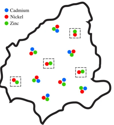
[image:10.595.204.401.390.486.2]The gap gene network is responsible for the segmented body pattern of theDrosophila melanogaster. During the blastoderm stage of the development of the body, different maternal gradients determine the polarity of the embryo along its anterior-posterior (A-P) axis (Perkins et al., 2006).
Figure 1: Drosophila body segmentation genes. Blue stripes correspond to hunchback, green stripes to knirps and red stripes to eve-skipped at cleavage cycle 14A, temporal class 3.
Maternal gradient interact with the so called trunk gap genes, includinghunchback (hb),Kr¨uppel (Kr),giant (gt), andknirps (kni), and this network of interactions establish the patterns of segmentation of the Drosophila.
Figure 1 shows the gene expression of the hunchback, the knirps and the eve-skipped genes in a color-scale intensity image. The image corresponds to cleavage cycle 14A, temporal class 3.7
The gap-gene network dynamics is usually represented using a set of coupled non-linear partial differential equations (Perkins et al., 2006; Gursky et al., 2004)
∂yd(x, t)
∂t =ζ(t)Pd(y(x, t))−λdyd(x, t) + Dd ∂2y
d(x, t) ∂x2 ,
whereyd(x, t)denotes the relative concentration of gap protein of thed-th gene at the space pointxand time pointt. The term Pd(y(x, t))accounts for production and it is a function, usually non-linear, of production of all other genes. The parameterλdrepresents the decay andDdthe diffusion rate. The functionζ(t)accounts for changes occurring during the mitosis, in which the transcription is off (Perkins et al., 2006).
We linearize the equation above by replacing the non-linear termζ(t)Pd(y(x, t))with the linear termPQq=1Sd,quq(x, t), whereSd,qare sensitivities which account for the influence of the latent forceuq(x, t)over the quantity of production of
gened. In this way, the new diffusion equation is given by
∂yd(x, t) ∂t =
X
∀q
Sd,quq(x, t)−λdyd(x, t) + Dd ∂2y
d(x, t) ∂x2 .
This expression corresponds to a second order non-homogeneous partial differential equation. It is also parabolic with one space variable and constant coefficients. The exact solution of this equation is subject to particular initial and boundary conditions. For a first boundary value problem with domain0 ≤x≤l, initial conditionyd(x, t= 0)equal to zero, and boundary conditions yd(x= 0, t)andyd(x =l, t)both equal to zero, the solution to this equation is given by Polyanin (2002); Butkovskiy and Pustyl’nikov (1993); Stakgold (1998)
yd(x, t) = Q X q=1 Sd,q Z t 0 Z l 0
uq(ξ, τ)Gd(x, ξ, t−τ)dξdτ,
where the Green’s functionGd(x, ξ, t)is given by
Gd(x, ξ, t) =
2
le
−λdt
∞
X
n=1
sinnπx
l sin nπξ l e
−Dd n2π2t
l2
.
We assume that the latent forcesuq(x, t)follow a Gaussian process with covariance function that factorizes across inputs dimensions, this is
kuq,uq(x, t, x′, t′) = exp −
(t−t′)2
ℓt q
2 !
exp −(x−x′) 2 ℓx q 2 ! ,
whereℓt
qrepresents the length-scale along the time-input dimension andℓxq the length-scale along the space input dimension. The covariance for the outputsyd(x, t),kfq
d,f
q d′(x, t, x
′, t′), is computed using the expressions for the Green’s function and
the covariance of the latent forces, in a similar fashion to equation (22), leading to
kfq
d,f
q d′(x, t, x
′, t′) = 4
ℓ2 ∞ X n=1 ∞ X m=1
kftq
d,f
q
d′(t, t
′)kx fq
d,f
q
d′(x, x
′), (26)
wherekt fq
d,f
q
d′(t, t
′)andkx fq
d,f
q
d′(x, x
′)are also kernel functions that depend on the indexesnandm. The kernel function
kt
fdq,fdq′(t, t′)is given by expression (10) andk x
fdq,fdq′(x, x′)is given by kxfq
d,f
q
d′(x, x
′) =C(n, m, ℓx
q) sin(ωnx) sin(ωmx′),
whereωn = nπℓ andωm= mπℓ . The termC(n, m, ℓxq)represents a function that depends on the indexesnandm, and on the length-scale of the space-input dimension. The expression forC(n, m, ℓx
q)is included in appendix B.
For completeness, we also include the cross-covariance between the outputs and the latent functions, which follows as
kfd,uq(x, t, x′, t′) =
2Sd,q l
∞
X
n=1
kt fd,uq(t, t
′)kx
fd,uq(x, x
′),
wherekt fd,uq(t, t
′)is given by expression (12), andkx
fd,uq(x, x
′)follows
kxfd,uq(x, x
′) = sin (w
nx)C(x′, n, ℓxq), whereC(x′, n, ℓx
q)is a function ofx′, the indexnand the length-scale of the space input dimension. The expression for C(x′, n, ℓx
q)is included in appendix C.
Prediction of gene expression data
We want to assess the contribution that a simple mechanistic assumption might bring to the prediction of gene expression data when compared to a covariance function that does not imply mechanistic assumptions.
case of the latent force model covariance in equations (21) and (22). If we makeGd(t−τ) =δ(t−τ)in equation (21), andkuq,uq(t, t′) =ku,u(t, t′)for all values ofq, we get
kfd,fd′(t, t
′) =
Q
X
q=1
Sd,qSd′,qku,u(t, t′).
Our purpose is to compare the prediction performance of the covariance above and the DROS covariance function. We use data from Perkins et al. (2006), in particular, we have quantitative wild-type concentration profiles for the protein products of giant and knirps at 9 time points and 58 spatial locations. We work with a gene at a time and assume that the outputs correspond to the different time points. This setup is very common in computer emulation of multivariate codes (see Conti and O’Hagan (2010); Osborne et al. (2008); Rougier (2008)) in which the MTGP model is heavily used. For the DROS kernel, we use 30 terms in each sum involved in its definition, in equation (26).
We randomly select 20 spatial points for training the models, this is, for finding hyperparameters according to the description of subsection 3.2. The other 38 spatial points are used for validating the predictive performance. Results are shown in table 2 for five repetitions of the same experiment. It can be seen that the mechanistic assumption included in the GP model considerably outperforms a traditional approach like MTGP, for this particular task.
Gene Method RMSE R2(%)
giant MTGP 26.56±0.30 81.12±0.01 DROS 2.00±0.35 99.78±0.01
[image:12.595.102.497.521.689.2]knirps MTGP 16.14±8.44 91.18±2.77 DROS 3.01±0.81 99.60±0.01
Table 2: RMSE and R2for protein data prediction
5.2
Diffusion in the Swiss Jura
The Jura data is a set of measurements of concentrations of several heavy metal pollutants collected from topsoil in a14.5
km2 region of the Swiss Jura. We consider a latent function that represents how the pollutants were originally laid down. As time passes, we assume that the pollutants diffuse at different rates resulting in the concentrations observed in the data set. We use a simplified version of the heat equation ofpvariables. Thep-dimensional non-homogeneous heat equation is represented as
∂yd(x, t) ∂t =
p
X
j=1
κd,j ∂2y
d(x, t) ∂x2
j
+ Φ(x, t),
wherep= 2is the dimension ofx, the measured concentration of each pollutant over space and time is given byyd(x, t), κd,j is the diffusion constant of outputd in direction p, and Φ(x, t) represents an external force, with x = {xj}pj=1.
Assuming the domainRp={−∞< xj <∞;j= 1, . . . , p}and initial condition prescribed by the set of latent forces,
u(x) =
Q
X
q=1
Sd,quq(x), att= 0,
the solution to the system (Polyanin, 2002) is then given by
yd(x, t) =
Z t
0 Z
Rp
Gd(x,x′, t, τ)Φ(x′, τ)dx′dτ+
Z
Rp
Gd(x,x′, t,0)u(x′)dx′, (27)
whereGq(x,x′, t, τ)is the Green’s function given by
Gd(x,x′, t, τ) =
1
2pπp/2qQp
j=1Td,j exp
−
p
X
j=1
(xj−x′j)2
4Td,j
,
withTd,j(t, τ) =κd,j(t−τ). The covariance function we propose here is derived as follows. In equation (27), we assume that the external forceΦ(x, t)is zero, following
yd(x, t) = Q
X
q=1
Sd,q
Z
Rp
We can write again the expression for the Green’s function as
Gd(x,x′, t) =
1
(2π)p/2qQp
j=12Td,j
exp − p X j=1
(xj−x′j)2
4Td,j
= 1
(2π)p/2qQp
j=1ℓd,j
exp − p X j=1
(xj−x′j)2
2ℓd,j
,
whereℓd,j = 2Td,j = 2κd,jt. The coefficientℓd,j is a function of time. In our model for the diffusion of the pollutant metals, we think of the data as a snapshot of the diffusion process. Consequently, we consider the time instant of this snapshot as a parameter to be estimated. In other words, the measured concentration is given by
yd(x) = Q X q=1 Sd,q Z Rp e
Gd(x,x′)uq(x′)dx′, (29)
whereGed(x,x′)is the Green’s functionGd(x,x′, t)that considers the variabletas a parameter to be estimated through ℓd,j. Expression forGed(x,x′)corresponds to a Gaussian smoothing kernel, with diagonal covariance. This is
e
Gd(x,x′) = |
Pd|1/2
(2π)p/2exp
−12(x−x′)⊤P
d(x−x′)
,
wherePdis a precision matrix, with diagonal form and entries{pd,j =ℓd,j1 }
p j=1.
If we take the latent function to be given by a GP with the Gaussian covariance function, we can compute the multiple output covariance functions analytically. The covariance function between the output functions,kfq
d,f
q
d′(x,x
′), is obtained
as
1 (2π)p/2|Pq
d,d′|1/2
exp
−12(x−x′)⊤Pqd,d′ −1
(x−x′)
,
wherePqd,d′ =P−
1
d +P−
1
d′ +Λ−q1, andΛqis the precision matrix associated to the Gaussian covariance of the latent force Gaussian process prior. The covariance function between the output and latent functions,kfq
d,uq(x,x
′), is given by
1 (2π)p/2|Pq
d|1/2
exp
−12(x−x′)⊤(Pqd)−1(x−x′)
,
wherePqd =P−d1+Λ−1
q .
Prediction of Metal Concentrations
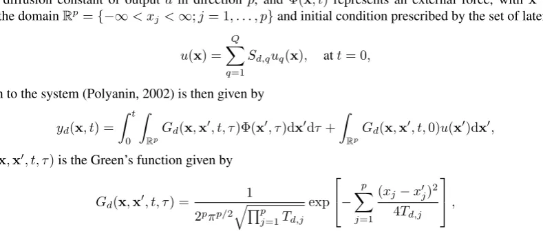
We used our model to replicate the experiments described in Goovaerts (pp. 248,249 1997) in which aprimary variable
(cadmium, cobalt, copper and lead) is predicted in conjunction with somesecondary variables(nickel and zinc for cadmium and cobalt; copper, nickel and zinc for copper and lead).8Figure 2 shows an example of the prediction problem. For several
sample locations we have access to the primary variable, for example cadmium, and the secondary variables, nickel and zinc. These sample locations are usually referred to as theprediction set. At some other locations, we only have access to the secondary variables, as it is shown in the figure by the squared regions. In geostatistics, this configuration of sample locations is known asundersampledorheterotopic, where usually a few expensive measurements of the attribute of interest are supplemented by more abundant data on correlated attributes that are cheaper to sample.
By conditioning on the values of the secondary variables at the prediction and validation sample locations, and the pri-mary variables at the prediction sample locations, we can improve the prediction of the pripri-mary variables at the validation locations. We compare results for the heat kernel with results from prediction using independent GPs for the metals, the multi-task Gaussian process and the semiparametric latent factor model. For our experiments we made use of ten repeats to report standard deviations. For each repeat, the data is divided into a different prediction set of259locations and different validation set of100locations. Root mean square errors and percentage of explained variance are shown in Tables 3 and 4, respectively.
Note from both tables that all methods outperform independent Gaussian processes, in terms of RMSE and explained variance. For one latent function (Q= 1), the Gaussian process with Heat kernel render better results than multi-task GPs (in this case, the multi-task GP is equivalent to the semiparametric latent factor model). However, when increasing the value of the latent forces to two (Q= 2), performances for all methods are quite similar. There is a still a gain in performance when using the Heat kernel, although the results are within the standard deviation. Also, when comparing the performances for the GP with Heat kernel using one and two latent forces, we notice that both measures are quite similar. In summary, the heat kernel provides a simplified explanation for the outputs, in the sense that, using only one latent force, we provide better performances in terms of RMSE and explained variance.
Nickel Zinc Cadmium
Figure 2: Sketch of the topsoil of Swiss Jura. Secondary variables like nickel and zinc help in the prediction of the primary variable cadmium, in the squared-regions.
Method Cadmium (Cd) Cobalt (Co) Copper (Cu) Lead (Pb)
IND GP 0.8353±0.0898 2.2997±0.1388 18.9616±3.4404 28.1768±5.8005
MTGP (Q= 1) 0.7638±0.1016 2.2892±0.1792 14.4179±2.7119 21.5861±4.1888
HEATK (Q= 1) 0.6773±0.0628 2.06±0.0887 13.1788±2.6446 17.9839±2.9450
MTGP (Q= 2) 0.6980±0.0832 2.1299±0.1983 12.7340±2.2104 17.9399±1.9981
SLFM (Q= 2) 0.6941±0.0834 2.172±0.1204 12.8935±2.6125 17.9024±2.0966
[image:14.595.82.525.330.416.2]HEATK (Q= 2) 0.6759±0.0623 2.0345±0.0943 12.5971±2.4842 17.5571±2.6076
Table 3: RMSE for pollutant metal prediction
Method Cadmium (Cd) Cobalt (Co) Copper (Cu) Lead (Pb)
IND GP 15.07±7.43 57.81±7.19 25.84±7.54 23.48±10.40
MTGP (Q= 1) 27.25±5.89 58.45±5.71 58.84±8.35 56.85±11.60
HEATK (Q= 1) 43.83±8.71 66.19±4.60 65.55±8.21 71.45±5.78
MTGP (Q= 2) 40.30±5.17 64.13±5.10 67.51±8.36 69.70±6.90
SLFM (Q= 2) 40.97±5.15 62.49±5.41 67.35±8.29 70.21±6.04
HEATK (Q= 2) 43.94±6.56 67.17±4.30 68.40±6.46 70.55±6.88
Table 4: R2for pollutant metal prediction
6
Related work
Differential equations are the cornerstone in a diverse range of engineering fields and applied sciences. However, their use for inference in statistics and machine learning has been less studied. The main field in which they have been used is known asfunctional data analysis(Ramsay and Silverman, 2005).
From the frequentist statistics point of view, the literature in functional data analysis has been concerned with the problem of parameter estimation in differential equations (Poyton et al., 2006; Ramsay et al., 2007): given a differential equation with unknown coefficients{Am}Mm=0, how do we use data to fit those parameters? Notice that there is a subtle difference
[image:14.595.110.491.448.534.2]Classical approaches to fit parameters θ of differential equations to observed data include numerical approximations of initial value problems and collocation methods (references Ramsay et al. (2007) and Brewer et al. (2008) provide reviews and detailed descriptions of additional methods).
The solution by numerical approximations include an iterative process in which given an initial set of parametersθ0and a
set of initial conditionsy0, a numerical method is used to solve the differential equation. The parameters of the differential
equation are then optimized by minimizing an error criterion between the approximated solution and the observed data. For exposition, we assume in equation (17) thatD= 1,Q= 1andS1,1= 1. We are interested in finding the solutiony(t)to
the following differential equation, with unknown parametersθ={Am}Mm=0,
DM0 y(t) =
M
X
m=0
AmDmy(t) =u(t),
In the classical approach, we assume that we have access to a vector of initial conditions,y0and data foru(t),u. We start
with an initial guess for the parameter vectorθ0and solve numerically the differential equation to find a solutioney. An
updated parameter vectorθeis obtained by minimizing
E(θ) =
N
X
n=1
kye(tn)−y(tn)k,
through any gradient descent method. To use any of those methods, we must be able to compute∂E(θ)/∂θ, which is equivalent to compute ∂y(t)/∂θ. In general, when we do not have access to∂y(t)/∂θ, we can compute it using what is known as thesensitivity equations(see Bard (1974), chapter 8, for detailed explanations), which are solved along with the ODE equation that provides the partial solutioney. Once a new parameter vectorθehas been found, the same steps are repeated until some convergence criterion is satisfied. If the initial conditions are not available, they can be considered as additional elements of the parameter vectorθand optimized in the same gradient descent method.
In collocation methods, the solution of the differential equation is approximated using a set of basis functions,{φi(t)}Ji=1,
this isy(t) =PJi=1βiφi(t). The basis functions must be sufficiently smooth so that the derivatives of the unknown func-tion, appearing in the differential equafunc-tion, can be obtained by differentiation of the basis representation of the solufunc-tion, this is,Dmy(t) =Pβ
iDmφi(t). Collocation methods also use an iterative procedure for fitting the additional parameters involved in the differential equation. Once the solution and its derivatives have been approximated using the set of basis functions, minimization of an error criteria is used to estimate the parameters of the differential equation. Principal differen-tial analysis (PDA) (Ramsay, 1996) is one example of a collocation method in which the basis functions aresplines. In PDA, the parameters of the differential equation are obtained by minimizing the squared residuals of the higher order derivative
DMy(t)and the weighted sum of derivatives
{Dmy(t)
}Mm=0−1, instead of the squared residuals between the approximated
solution and the observed data.
An example of a collocation method augmented with Gaussian process priors was introduced by Graepel (2003). Graepel starts with noisy observations,yb(t), of the differential equationDM
0 y(t), such thatyb(t)∼ N(DM0 y(t), σy). The solution y(t) is expressed using a basis representation,y(t) = Pβiφi(t). A Gaussian prior is placed over β = [β1, . . . , βJ], and its posterior computed under the above likelihood. With the posterior overβ, the predictive distribution foryb(t∗)can be readily computed, being a function of the matrix DM0 Φ with elements{D0Mφi(tn)}N,Jn=1,i=1. It turns out that
prod-ucts DM0 Φ DM0 Φ⊤ that appear in this predictive distribution have individual elements that can be written using the sum PJi=1DM
0 φi(tn)D0Mφi(tn′) = D0M,tDM0,t′ PJ
i=1φi(tn)φi(tn′)or, using a kernel representation for the inner prod-uctsk(tn, tn′) =PJi=1φi(tn)φi(tn′), askDM
0,t,DM0,t′(tn, tn′), where this covariance is obtained by takingD M
0 derivatives of
k(t, t′)with respect totandDM
0 derivatives with respect tot′. In other words, the result of the differential equationD0My(t)
is assumed to follow a Gaussian process prior with covariancekDM
0,t,DM0,t′(t, t
′). An approximated solutionye(t)can be
com-puted through the expansionye(t) =PNn=1αnkDM
0,t′(t, tn), whereαnis an element of the vector(KD0M,t,DM0,t′+σyIN)
−1by,
whereKDM
0,t,DM0,t′ is a matrix with entrieskDM0,t,DM0,t′(tn, tn′)andbyare noisy observations ofD M
0 y(t).
Although, we presented the above methods in the context of linear ODEs, solutions by numerical approximations and col-location methods are applied to non-linear ODEs as well.
point by means of a Taylor series expansion (Thompson, 2009),
y(t) =
∞
X
j=0
y(j)(a)
j! (t−a)
j,
withathe equilibrium point. For a finite value of terms, the linearization above can be seen as a regression problem in which the covariates correspond to the terms(t−a)j and the derivativesy(j)(a)as regression coefficients. The derivatives are
assumed to follow a Gaussian process prior with a covariance function that is obtained ask(j,j′)
(t, t′), where the superscript
jindicates how many derivative ofk(t, t′)are taken with respect totand the superscriptj′indicates how many derivatives of
k(t, t′)are taken with respect tot′. Derivatives are then estimated a posteriori through standard Bayesian linear regression.
An important consequence of including derivative information in the inference process is that the uncertainty in the posterior prediction is reduced as compared to using only function observations. This aspect of derivative information have been exploited in the theory of computer emulation to reduce the uncertainty in experimental design problems (Morris et al., 1993; Mitchell and Morris, 1994).
Gaussian processes have also been used to model the outputy(t)at timetkas a function of itsLprevious samples{y(t− tk−l)}Ll=1, a common setup in the classical theory of systems identification (Ljung, 1999). The particular dependency
y(t) =g({y(t−tk−l)}Ll=1), whereg(·)is a general non- linear function, is modelled using a Gaussian process prior and the
predicted value for the outputy∗(tk)is used as a new input for multi-step ahead prediction at timestj, withj > k(Kocijan et al., 2005). Uncertainty abouty∗(tk)can also be incorporated for predictions of future output values (Girard et al., 2003). On the other hand, multivariate systems with Gaussian process priors have been thoroughly studied in the spatial analysis and geostatistics literature (Higdon, 2002; Boyle and Frean, 2005; Journel and Huijbregts, 1978; Cressie, 1993; Goovaerts, 1997; Wackernagel, 2003). In short, a valid covariance function for multi-output processes can be generated using the linear model of coregionalization (LMC). In the LMC, each outputyd(t)is represented as a linear combination of a series of basic processes{uq}Qq=1, some of which share the same covariance functionkuq,uq(t, t′). Both, the semiparametric latent
factor model (Teh et al., 2005) and the multi-task GP (Bonilla et al., 2008) can be seen as particular cases of the LMC ( ´Alvarez et al., 2011b). Higdon (2002) proposed the direct use of a expression (18) to obtain a valid covariance function for multiple outputs and referred to this kind of construction as process convolutions. Process convolutions for constructing covariances for single output GP had already been proposed by Barry and Ver Hoef (1996); Ver Hoef and Barry (1998). Calder and Cressie (2007) reviews several extensions of the single process convolution covariance. Boyle and Frean (2005) introduced the process convolution idea for multiple outputs to the machine learning audience. Boyle (2007) developed the idea of using impulse responses of filters to representGd(t, s), assuming the processv(t)was white Gaussian noise. Independently, Murray-Smith and Pearlmutter (2005) also introduced the idea of transforming a Gaussian process prior using a discretized version of the integral operator of equation (18). Such transformation could be applied for the purposes of fusing the information from multiple sensors (a similar setup to the latent force model but with a discretized convolution), for solving inverse problems in reconstruction of images or for reducing computational complexity working with the filtered data in the transformed space (Shi et al., 2005).
There has been a recent interest in introducing Gaussian processes in the state space formulation of dynamical systems (Ko et al., 2007; Deisenroth et al., 2009; Turner et al., 2010) for the representation of the possible nonlinear relationships between the latent space and between the latent space and the observation space. Going back to the formulation of the dimensionality reduction model, we have
utn=g1(utn−1) +η,
ytn=g2(utn) +ǫ,
where η andξ are noise processes and g1(·) andg2(·) are general non-linear functions. Usuallyg1(·)and g2(·) are
unknown, and research on this area has focused on developing a practical framework for inference when assigning Gaussian process priors to both functions.
Finally, it is important to highlight the work of Calder (Calder, 2003, 2007, 2008) as an alternative to multiple-output modeling. Her work can be seen in the context of state-space models,
utn=utn−1+η,
ytn =Gtnutn+ǫ,
whereytnandutn are related through a discrete convolution over an independent spatial variable. This is, for a fixedtn,
ytn
d (s) =
P
q
P
iG tn
7
Conclusion
In this paper we have presented a hybrid approach to modelling that sits between a fully mechanistic and a data driven ap-proach. We used Gaussian process priors and linear differential equations to model interactions between different variables. The result is the formulation of a probabilistic model, based on a kernel function, that encodes the coupled behavior of several dynamical systems and allows for more accurate predictions. The implementation of latent force models introduced in this paper can be extended in several ways, including:
Non-linear Latent Force Models. If the likelihood function is not Gaussian the inference process has to be accomplished in a different way, through a Laplace approximation (Lawrence et al., 2007) or sampling techniques (Titsias et al., 2009).
Cascaded Latent Force Models. For the above presentation of the latent force model, we assumed that the covariances kuq,uq(t, t′)were squared-exponential. However, more structured covariances can be used. For example, in Honkela et al.
(2010), the authors use a cascaded system to describe gene expression data for which a first order system, like the one presented in subsection 3.1, has as inputsuq(t)governed by Gaussian processes with covariance function (10).
Stochastic Latent Force Models. If the latent forcesuq(t)are white noise processes, then the corresponding differential equations are stochastic, and the covariances obtained in such cases lead to stochastic latent force models. In ´Alvarez et al. (2010), a first-order stochastic latent force model is employed for describing the behavior of a multivariate financial dataset: the foreign exchange rate with respect to the dollar of ten of the top international currencies and three precious metals.
Switching dynamical Latent Force Models. A further extension of the LFM framework allows the parameter vectorθ to have discrete changes as function of the input time. In ´Alvarez et al. (2011a) this model was used for the segmentation of movements performed by a Barrett WAM robot as haptic input device.
Acknowledgments
DL has been partly financed by Comunidad de Madrid (project PRO-MULTIDIS-CM, S-0505/TIC/0233), and by the Span-ish government (CICYT project TEC2006-13514-C02-01 and researh grant JC2008-00219). MA and NL have been fi-nanced by a Google Research Award and EPSRC Grant No EP/F005687/1 “Gaussian Processes for Systems Identification with Applications in Systems Biology”. MA also acknowledges the support from the Overseas Research Student Award Scheme (ORSAS), from the School of Computer Science of the University of Manchester and from the Universidad Tec-nol´ogica de Pereira, Colombia.
A
Preprocessing for the mocap data
For selecting the subset of angles for each of the motions for the golf-swing movement and the walking movement, we use as performance measure the signal-to-noise ratio obtained in the following way. We train a GP regressor for each output, employing a covariance function that is the sum of a squared exponential kernel and a white Gaussian noise,
σ2
Sexp
−(x−x′)
2
2ℓ2
+σ2
Nδ(x,x′),
whereσ2
S andσ2N are variance parameters, and δ(x,x′)is the Dirac delta function. For each output, we compute the signal-to-noise ratio as10 log10(σS2/σ2N).
B
Expression for
C
(
n, m, ℓ
x)
For simplicity, we assumeQ= 1and writeℓx
q =ℓx. The expression forC(n, m, ℓx)is given by
C(n, m, ℓx) =
Z l
0 Z l
0
sin (wnξ) sin (wmξ′)e
−(ξ−ξ′)
2
ℓ2
x
dξ′dξ.
The solution of this double integral depends upon the relative values ofnandm. Ifn6=m, andnandmare both even or both odd, then the analytical expression forC(n, m, ℓx)is
ℓxl √π(m2−n2)
whereI[·]is an operator that takes the imaginary part of the argument andW(m, ℓx)is given by
W(m, ℓx) =w(jz1γm)−e−(
l
ℓx)
2
e−γmlw(jzγm
2 ),
beingzγm
1 =
ℓxγm
2 ,z
γm
2 = ℓlx +
ℓxγm
2 andγm=jωm.
The termC(n, m, ℓx)is zero if, forn6=m,nis even andmis odd or viceversa.
Finally, whenn=m, the expression forC(n, n, ℓx)follows as
ℓx√π l
2
RW(n, ℓx)− I[W(n, ℓx)]
hℓ2
xnπ
2l2 + 1
nπ i
+ℓ 2
x
2 h
e−(ℓxl)
2
cos(nπ)−1i,
whereR[·]is an operator that takes the real part of the argument.
C
Expression for
C
(
x
′, n, ℓ
x)
As in appendix B, we assumeQ= 1andℓx
q =ℓx. The expressionC(x′, n, ℓx)is as ℓx√π
2 I
e−
x′ −l
ℓx
2
eγnlw(jzγn,x′
2 )−e−
x′
ℓx
2
w(jzγn,x′
1 )
,
withzγn,x′
1 = x
′ ℓx +
ℓxγn
2 ,z
γn,x′
2 = x
′−l ℓx +
ℓxγn
2 ,γn = jωn andI[·]is an operator that takes the imaginary part of the
argument.
References
Mauricio A. ´Alvarez and Neil D. Lawrence. Sparse convolved Gaussian processes for multi-output regression. In Koller et al. (2009), pages 57–64.
Mauricio A. ´Alvarez, David Luengo, and Neil D. Lawrence. Latent Force Models. In van Dyk and Welling (2009), pages 9–16.
Mauricio A. ´Alvarez, David Luengo, Michalis K. Titsias, and Neil D. Lawrence. Efficient multioutput Gaussian processes through variational inducing kernels. In Teh and Titterington (2010), pages 25–32.
Mauricio A. ´Alvarez, Jan Peters, Bernhard Sch¨olkopf, and Neil D. Lawrence. Switched latent force models for movement segmentation. InNIPS, volume 24, pages 55–63. MIT Press, Cambridge, MA, 2011a.
Mauricio A. ´Alvarez, Lorenzo Rosasco, and Neil D. Lawrence. Kernels for vector-valued functions: a review. Technical report, University of Manchester, Massachusetts Institute of Technology and University of Sheffield, 2011b. Available at
http://arxiv.org/pdf/1106.6251v1.
Yonathan Bard. Nonlinear Parameter Estimation. Academic Press, first edition, 1974.
Ronald Paul Barry and Jay M. Ver Hoef. Blackbox kriging: spatial prediction without specifying variogram models.Journal of Agricultural, Biological and Environmental Statistics, 1(3):297–322, 1996.
Sue Becker, Sebastian Thrun, and Klaus Obermayer, editors.NIPS, volume 15, Cambridge, MA, 2003. MIT Press.
Edwin V. Bonilla, Kian Ming Chai, and Christopher K. I. Williams. Multi-task Gaussian process prediction. In John C. Platt, Daphne Koller, Yoram Singer, and Sam Roweis, editors,NIPS, volume 20, Cambridge, MA, 2008. MIT Press.
Phillip Boyle.Gaussian Processes for Regression and Optimisation. PhD thesis, Victoria University of Wellington, Welling-ton, New Zealand, 2007.
Phillip Boyle and Marcus Frean. Dependent Gaussian processes. In Lawrence Saul, Yair Weiss, and L´eon Bouttou, editors,
NIPS, volume 17, pages 217–224, Cambridge, MA, 2005. MIT Press.