City, University of London Institutional Repository
Citation
:
Bilinski, P. and Lyssimachou, D. (2014). Risk Interpretation of the CAPM's Beta: Evidence from a New Research Method. Abacus, 50(2), pp. 203-226. doi:10.1111/abac.12028
This is the accepted version of the paper.
This version of the publication may differ from the final published
version.
Permanent repository link:
http://openaccess.city.ac.uk/7556/Link to published version
:
http://dx.doi.org/10.1111/abac.12028Copyright and reuse:
City Research Online aims to make research
outputs of City, University of London available to a wider audience.
Copyright and Moral Rights remain with the author(s) and/or copyright
holders. URLs from City Research Online may be freely distributed and
linked to.
City Research Online: http://openaccess.city.ac.uk/ [email protected]
PAWEL BILINSKI AND DANIELLE LYSSIMACHOU
b1
The Risk Interpretation of the CAPM’s Beta:
Evidence from a New Research Method
This study tests the validity of using the CAPM beta as a risk control in cross-sectional accounting and finance research. We recognize that high risk stocks should experience either very good or very bad returns more frequently compared to low risk stocks, i.e. high risk stocks should cluster in the tails of the cross-sectional return distribution. Building on this intuition, we test the risk interpretation of the CAPM’s beta by examining if high beta stocks are more likely than low beta stocks to experience either very high or very low returns. Our empirical results indicate that beta is a strong predictor of large positive and large negative returns, which confirms that beta is a valid empirical risk measure and that researchers should use beta as a risk control in empirical tests. Further, we show that because the relation between beta and returns is U-shaped, i.e. high betas predict both very high and very low returns, linear cross-sectional regression models, e.g. Fama-MacBeth regressions, will fail on average to reject the null hypothesis that beta does not capture risk. This result explains why previous studies find no significant cross-sectional relation between beta and returns.
Key words: Market beta; New research method; Empirical accounting and finance
research.
PAWEL BILINSKI ([email protected]) and DANIELLE LYSSIMACHOU ([email protected]) are Associate Professors of Accounting at Cass Business School, City University London.
2 INTRODUCTION
The capital asset pricing model (CAPM) of Sharpe (1964) and Lintner (1965) lies at the heart of
empirical accounting and finance research.1 Early empirical tests by Black et al. (1972), Blume and
Friend (1973) and Fama and MacBeth (1973) show that beta explains the cross-section of stock
returns. However, a plethora of subsequent studies, including Lakonishok and Shapiro (1986) and
Ritter and Chopra (1989) find no evidence of a significant cross-sectional relation between beta and
returns. Fama and French (1992) provide the most convincing evidence challenging beta’s ability to
explain the cross-section of stock returns. They show that beta sorts produce no significant return
spread, but that two other characteristics, firm size and the book-to-market ratio, capture the
cross-section of asset returns. They obtain similar conclusions using Fama-MacBeth regressions.
To date, the accounting and finance literature has not arrived at a satisfactory conclusion on
the validity of using the CAPM’s beta as a risk control in empirical research.2 However, without
clear-cut resolutions, discarding beta as a risk control can lead to asset pricing model
misspecification and, consequently, erroneous conclusions in empirical tests.3 This paper uses a
simple test to examine if market beta captures risk and, consequently, if researchers should use beta
as a risk control in empirical tests. The framework we propose also explains why previous studies
have failed to reject the null hypothesis that beta does not capture the cross-section of stock returns.
The departure point for our tests is the intuition that risky stocks should experience very
good or very bad returns more frequently compared to low risk stocks, i.e. risky stocks should
concentrate in the tails of the cross-sectional return distribution. Building on this insight, a test of
whether high beta stocks are more risky is equivalent to testing if high beta stocks tend to experience
very high and very low returns more often than low beta stocks.4 We operationalize this test with
two logistic regressions, one that predicts large positive returns and the other that predicts large
3 market betas in both regressions should be significant and positive. The two regressions control for
common empirical risk factors, such as firm size and the book-to-market ratio, to examine if these
risk proxies subsume beta’s role in explaining the return cross-section (Fama and French, 1992,
1993).
We start the analysis by replicating previous evidence that beta shows no association with the
return cross-section. A simple portfolio analysis that sorts stocks into deciles based on beta shows a
flat relation between beta and monthly returns, consistent with previous evidence (Lakonishok and
Shapiro, 1986; Ritter and Chopra, 1989; Fama and French, 1992). Further, we find no relation
between beta and returns when we use pooled cross-sectional OLS regressions or the
Fama-MacBeth method. Together, this confirms previous conclusions that standard research methods
produce no evidence of a cross-sectional association between beta and stock returns.
Next, we test if high beta stocks are more likely than low beta stocks to experience large
negative and large positive returns. We start by splitting stocks into deciles based on their monthly
returns. This allows us to identify the tails of the cross-sectional return distribution. Consistent with
our prediction, we find that high beta stocks tend to cluster among stocks with large positive and
large negative returns.
In subsequent analysis, we use two logistic regressions to test if high betas predict large
negative and large positive returns. As a starting point, we use arbitrary cut-off points to define the
dependent variables for the two logistic models. Specifically, the dependent variable in the regression
predicting high returns takes the value of one if the stock’s monthly returns are higher than 20%,
and zero otherwise. For the logistic model testing if high beta stocks are more likely to experience
large negative returns, the dependent variable is one if monthly returns are lower than −15%, and
zero otherwise.5 Multivariate logistic regressions show that the coefficients on betas are positive and
4 favorable and unfavorable outcomes. This evidence supports the prediction that beta captures risk
and that researchers should use beta as a risk control in empirical tests.
Our conclusion that beta reflects risk is robust to a battery of sensitivity tests. First, we show
that our conclusion is not sensitive to the specification of the cut-off points we use to define the
dependent variables in the two logistic models, and the conclusion remains unchanged when we use
past stock returns to construct the dependent variables in the logistic regressions.6 Second, we show
that beta predicts large positive and large negative returns when we use Dimson’s (1979) beta to
control for stock thin trading and the resultant downward bias in beta coefficients, when we use
betas estimated at portfolio-level rather than at firm-level to control for the errors-in-variables
problem, and when we estimate betas over a five-year rather than a three-year period. The latter test
addresses the problem of beta’s instability over time (Bos and Newbold, 1984). Finally, as part of the
sensitivity analysis, we also show that our inferences remain the same when we use non-parametric
quantile regressions to test for the association between beta and large positive and negative returns.
Quantile regressions examine the association between beta and returns for various cut-off points of
the return distribution. Standard OLS/Fama-MacBeth methods only estimate if beta explains the
conditional mean return. Quantile regressions show that beta is a strong predictor of returns in the
top and the bottom decile of the return distribution, which supports our main conclusions.
Our study offers two important contributions to the literature. First, using a simple research
framework that focuses on the tails of the cross-sectional return distribution, we provide robust
evidence that beta captures risk that drives stock returns. This adds important new evidence to the
literature that examines the validity of using beta as a risk control in empirical accounting and
finance research. Our testing framework has numerous advantages. It is very simple to implement, it
builds on the intuition of ‘what a risky stock is’, and avoids imposing a linear constraint on the
5 method. The approach does not increase the likelihood of falsely rejecting the null hypothesis that
beta does not reflect risk because for beta to associate with risk, coefficients on betas in both
predictive regressions need to be significant and have the same sign.7
Second, our study explains why standard portfolio analysis, and cross-sectional
OLS/Fama-MacBeth regressions have low power to reject the null hypothesis that beta does not explain the
return cross-section. We show that high beta stocks experience large positive and large negative
returns more often compared to low beta stocks. Standard cross-sectional sorts that allocate high
beta stocks into a single portfolio will combine stocks with positive and negative returns producing
only average portfolio returns. In other words, standard sorts on beta impose a linear constraint on
the relation between beta and returns, whereas this relation is U-shaped. This produces weak or no
evidence on the cross-sectional association between beta and returns using standard sorts on beta. In
a similar way, cross-sectional OLS/Fama-MacBeth regressions impose a linear relation between beta
and returns, which biases beta coefficients towards zero. We advocate that future research uses
either logit models or quantile regressions focused on the tails of the return distribution in asset
pricing tests as both models accommodate the U-shaped relation between the risk proxy (such as
market beta) and stock returns.
A NEW APPROACH FOR TESTING THE RISK INTERPRETATION OF BETA
This paper uses a new method to examine if cross-sectional differences in market beta reflect
differences in risk. We build on the intuition that risky stocks should concentrate in the tails of the
cross-sectional return distribution, i.e. risky stocks should be more likely, on average, to experience
large positive or large negative returns compared to low risk stocks. Why is it that the case?
Assume that expected excess stock returns are generated according to the CAPM:
( )it ft i[ ( mt) ft]
6
mt
R is the market return, and Betai measures the sensitivity of stock’s i returns to the expected market risk premium and captures systematic risk. The realized stock return for firm i equals
[ ]
it ft i mt ft it
r r Beta R r , where it is the stock’s idiosyncratic return component that has
zero-expectation and is uncorrelated with the market premium.
Now consider two stocks, A and B, where stock A has higher systematic risk than stock B,
i.e. BetaA>BetaB. What is the relation between beta and the frequency of realized returns on stocks A
and B being (1) higher than a return rU, and (2) lower than a return rL, where rUrepresents a relatively
large positive return and rL a relatively large negative return? As idiosyncratic shocks are random, at
any given date t, the absolute return for stock A is likely to be higher than for stock B for any realization of the market premium. Further, the larger the absolute magnitudes of the cut-off points
rU and rL, the ‘more risky’ a stock has to be for the realized return to be higher than rU or lower than rL, i.e. the idiosyncratic component it becomes increasingly less important in determining if returns
for stocks A and B will beat benchmarks rU and rL. Together, this means that the likelihood of a
realized return higher than rU or lower than rL is on average higher for the more risky stock A than
for stock B, particularly for large magnitudes of rU and rL. A corollary of the above discussion is that
high beta stocks will tend to cluster in the tails of the cross-sectional return distribution, i.e. among
stocks experiencing large negative and large positive returns. If beta is not a proper measure of risk
and returns are not generated by the CAPM, there should be no systematic positive relation between
beta and the frequency of relatively large and low returns.8
An important conclusion that follows from the above discussion is that a test of beta as a
risk measure is equivalent to testing whether high beta stocks tend to concentrate in the tails of the
cross-sectional return distribution. Consequently, one can implement a simple test of whether
7 the other predicting large negative returns from beta. Specifically, the two predictive regressions
have the form:
0 0 0 0
_ (High ret)
P Beta Controls u (1)
1 1 1 1
( _ )
P Low ret Beta Controls u (2)
where the dependent variable, High_ret (Low_ret) equals one if a firm’s return is higher (lower) than a set benchmark, and zero otherwise.9
To define the dependent variables in models (1) and (2), we measure returns each month
over a one-year period starting at the end of the fourth month after the fiscal year-end.10 As a
starting point, we use arbitrary cut-off points of 20% and −15% to define the dependent variables in
the two logit models. Specifically, the dependent variable for model (1) is one if the stock’s monthly
return is higher than 20%, and zero otherwise. For model (2), the dependent variable is one if the
monthly return is below −15%, and zero otherwise. Kothari and Shanken (1997) report that the
annual equally-weighted return on the CRSP index is 12.5% over 1941–1991, or 0.99% per month.
This means that our breakpoints of 20% and −15% should be successful in identifying stocks in the
tails of the cross-sectional return distribution. In robustness tests we also consider other cut-off
points to test the sensitivity of our results to the specification of the dependent variables.
Under the assumption that returns and betas are jointly normally distributed, and that betas
capture risk, we would expect both β0 and β1 from models (1) and (2) to be significant and similar in
magnitude. However, since the normality assumption is unlikely to hold (Ané and Geman, 2000;
Chung et al., 2006), we impose a weaker condition that beta reflects risk if β0 and β1 are non-zero and
have the same sign. If the coefficients on beta are varying in sign in the two models or beta is
significant in only one regression, we conclude that beta is unlikely to capture risk. If both β0 and β1
8 Our main tests for models (1) and (2) use pooled cross-sectional samples and we adjust for
the cross-sectional and time-series dependence among observations using dual-clustered standard
errors on firm and year-month. For robustness purposes and to ensure comparability with previous
studies, we also use the Fama-MacBeth method. The Fama-MacBeth approach controls for the
time-series dependence among observations, but ignores the cross-sectional correlation among
stocks.12
Market beta and control variables
We estimate market beta (Beta) for each stock over a 3-year period ending four months after the fiscal year-end using the CAPM. We require a minimum of 30 observations for a stock to be
included in the beta computation. For each regression, we also calculate the mean squared error to
capture the residual pricing error, Resid. This is because large positive or large negative returns can be driven by the stock’s idiosyncratic risk component that is captured by the CAPM’s error term. A
positive correlation between beta and the error term can produce a significant coefficient on beta in
our regressions, even if beta does not capture risk.
The control variables in models (1) and (2) include firm characteristics commonly
associated with stock returns. Following Fama and French (1992), we include firm market
capitalization (MV) and the book-to-market ratio (B/M).13 Firm market capitalization equals the
number of shares outstanding multiplied by the end-of-month stock price measured four months
after the fiscal year-end. We follow Daniel and Titman (2006) and define book equity as the
difference between total shareholders’ equity and the preferred stock value. The book-to-market
ratio equals the ratio of book equity over market capitalization measured at the end of the previous
9 Other return predictors include stock return momentum (MOM), which is the difference between the stock’s and the market’s six-month buy-and-hold returns ending four months after the
fiscal year-end. We use firm age (Age), which is the difference between the firm’s previous fiscal year-end and the firm’s first appearance on CRPS files, to capture the stock’s information
uncertainty. Zhang (2006) proposes that firms with a long listing history have more information
available to investors to help with the stock’s valuation.14 Finally, we use a dummy variable to
identify loss making firms (Loss). Specifically, Loss takes a value of one if the net income for the previous fiscal year is negative, and is zero otherwise. Loss making firms are more difficult to value
(Watts and Zimmerman, 1986; Collins et al., 1997) and subject to higher financial distress (Ohlson, 1980).15 All explanatory variables are winsorized at the 1st and 99th percentiles.
DATA AND DESCRIPTIVE STATISTICS
We obtain returns on ordinary common shares from CRSP and accounting information from the
CRSP/Compustat merged database. The risk free rate and the market return required to estimate
betas are collected from Kenneth French’s website. Our sample includes all firms listed on
NYSE/AMEX/Nasdaq from January 1975 till December 2005.16 Following Fama and French
(1992), we retain only stocks with positive book values of equity. To avoid the delisting bias
(Shumway, 1997; Shumway and Warther, 1999), we include delisting returns. When a delisting return
is missing, we assume a return of −1 for delisting due to liquidation (CRSP codes 400–490), −0.33
for performance related delisting (500 and 520–584), and zero otherwise. Our final sample includes
1,015,320 firm-month observations.
Panel A of Table 1 presents the descriptive statistics. The mean monthly return is 1.6%
and it ranges from −6.1% in the lower quartile to 7.4% in the upper quartile. The sample beta is 1.05
10 the average firm has a market capitalization of over $1,035m. The mean past six-month abnormal
return equals 3.7% and is consistent with the average beta being higher than one. The average firm
age in the sample is 15.661 years and 24.1% of firms reported a negative net income in the previous
fiscal year.
[Insert Table 1 here]
Panel B reports the Pearson correlation coefficients. The magnitudes of the correlations are
low on average. Importantly, all pairwise correlations are far below 0.8, which is a rule-of-thumb
indicator for potential multicollinearity problems. The strongest correlations are between Beta and
Resid (0.366) and Resid and the indicator variable for loss-making firms (0.430).
PORTFOLIO ANALYSIS
As a simple test of the relation between beta and stock returns, Panel A of Table 2 presents the
results from portfolio analysis that allocates stocks into beta deciles. Specifically, each month we sort
stocks into beta deciles (High beta to Low beta). Subsequently, we calculate the mean monthly return and the average beta for each decile. Consistent with earlier findings, the relation between portfolio
betas and portfolio returns is flat and the difference in mean returns between portfolios of high and
low beta stocks is indistinguishable from zero (result untabulated). The latter evidence is particularly
striking given the very large difference in mean betas between the portfolios of high and low beta
stocks (2.707).
[Insert Table 2 here]
We predict that risky stocks should concentrate in the tails of the cross-sectional return
distribution. To test whether stocks with high positive or high negative returns have higher betas,
11 calculate the mean return and mean beta for each portfolio. Consistent with our prediction, stocks
with the most positive and the most negative monthly returns tend to have higher betas. Specifically,
the decile portfolio with the most positive returns has a mean beta of 1.206, the medium deciles 5
and 6 have mean betas of 0.924, and the decile with the most negative returns has a mean beta of
1.284. In unreported results we find that the differences in betas between the high and low return
deciles and the medium return deciles 5 and 6 are significant at less than 1% level. This confirms
that the relation between returns and market beta is U-shaped, i.e. high beta stocks tend to
experience high and low returns more often than low beta stocks.
Fama and French (1992) report that beta sorts closely replicate sorts on firm size because of
the negative relation between beta and firm market capitalization. This means that our finding in
Panel B of Table 2, that high beta stocks tend to have large positive and negative returns more often
than low beta stocks, may be simply capturing the size effect. To address this, Panel C repeats the
analysis from Panel B where we first split stocks into deciles based on their size. Each size decile is
then subdivided into ten portfolios based on stocks’ monthly returns. The portfolio formation is
repeated each month. For each size decile we find that high beta stocks cluster in the tails of the
return distribution. This confirms that clustering of high beta stocks in the tails of the
cross-sectional return distribution is independent of the size effect.17
In unreported results we find that our conclusion that high beta stocks cluster in the tails of
the return distribution remains unchanged when we use betas estimated at portfolio level, instead of
individual stock betas.18 Individual firm betas may be subject to an estimation error (the
errors-in-variables problem), which can attenuate the relation between beta and returns (Kim, 1995; Amihud
et al., 1993). The evidence that using portfolio betas leads to similar conclusions as when using individual stock betas is consistent with the conclusions in Fama and French (1992, p. 432) that
12 βs [betas estimated at firm level]. We take this to be evidence that the pre-ranking β sort captures the
ordering of true post-ranking βs.’. Fama and French (1992) also conclude that allocating portfolio
betas to individual stocks reduces the power of tests to identify a positive correlation between beta
and returns. Consequently, we use individual stock betas in the remaining analysis and use portfolio
betas in sensitivity tests.19
REGRESSION ANALYSIS
Pooled OLS and Fama Macbeth Regressions
Next we examine the relation between beta and returns in a regression framework. Fama and French
(1992) conclude that beta shows no association with stock returns over the period 1962–1989. As
our sample period ends in 2005, we first examine if using a more recent sample period, beta
continues to have an insignificant cross-sectional relation with returns. Consistent with past studies,
our cross-sectional regression model takes the form:
0 1 2 3 4 5 6 7
8 29
8 17
0 0
/ ln ln
it it it it it it it
k k it
k k
r beta Resid B M MV MOM Age Loss
Industry effect Year effect (3)
where ln indicates a logarithmic transformation of a variable and Industry effect and Year effect are industry and year dummies. Industry dummies are based on the two-digit SIC codes. We estimate
model (3) using pooled OLS and we cluster standard errors on firm and year-month to control for
the cross-sectional and time-series dependence of observations. For comparability with previous
studies, we also use Fama-MacBeth regressions to estimate model (3).20 We present the regression
results in Table 3.21
[Insert Table 3 here]
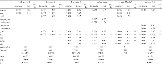
Table 3 shows that using pooled OLS regressions, the coefficient on market beta is
13 for firm size and the book-to-market ratio (Regression 2), and when we include other return predictors as specified in model (3) (Regression 3). The coefficient on beta remains insignificant when we use betas estimated at portfolio level in model (3) (Portfolio betas), and when we use the Fama-MacBeth approach (Fama MacBeth). Finally, our conclusion that beta has no power to explain the cross-section of stock returns remains unchanged when we use Dimson’s (1979) beta in model (3) (Dimson beta). We calculate Dimson betas as the sum of beta coefficients from regressions of excess stock returns
on the lead, current and lagged market premium. Dimson betas adjust for thin trading bias in beta
estimates (Dimson, 1979; Dimson and Marsh, 1983).
With respect to the control variables, we document a positive and significant coefficient on
the B/M ratio and a negative coefficient on firm size in all specifications of regression (3). This
confirms the evidence in Fama and French (1992) that small and high B/M stocks tend to have
higher returns than large and low B/M stocks. We also find evidence that stock return momentum
and firm age correlate with stock returns. Overall, our analysis in Table 3 confirms that beta shows
no significant association with stocks returns.
Logistic Regressions
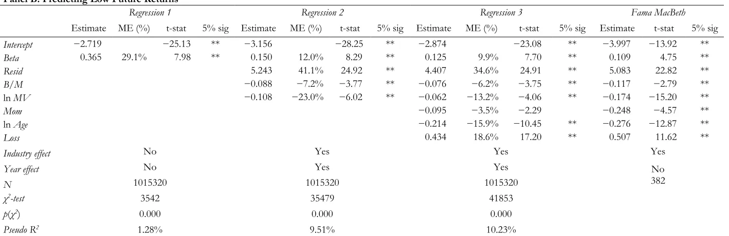
Table 4 reports regression results for logistic models (1) and (2). Panel A reports results for model
(1) and Panel B for model (2). On its own, beta is a strong predictor of large positive and large
negative returns (Regression 1). Consistent with our prediction, the coefficients on betas in the two logistic regressions are positive and significant, and largely similar in magnitude (0.329 for model (1)
and 0.365 for model (2)). A one standard deviation change in beta increases the likelihood of large
positive (negative) returns by 26.2% (29.1%), which confirms that beta has an economically
significant ability to predict large positive and negative return outcomes. Controlling for the B/M
14 and negative returns. The coefficients on betas remain significant and positive for the full
specification of the two logit models (Regression 3), and when we use the Fama-MacBeth approach (Fama MacBeth). Together, the results in Table 4 confirm our prediction that beta captures risk.
[Insert Table 4 here]
With respect to the control variables, we find that firms with large values of the pricing error
Resid tend to experience large positive and negative returns more often than firms with smaller pricing errors. This is consistent with Fu (2009), who build on the evidence that investors do not
hold well diversified portfolios and argue that under-diversified investors may require a premium for
bearing idiosyncratic risk. Further, smaller, younger firms and loss making firms cluster in the tails
of the cross-sectional return distribution. This is consistent with the risk interpretation of these
variables. The coefficients on return momentum and the B/M ratio are indistinguishable from zero
in model (1) that predicts large positive returns and are negative in model (2) that predicts low
returns. Together, this shows that high momentum stocks and high B/M stocks do not cluster
systematically in the tails of the cross-sectional return distribution, which suggests that they are
unlikely to reflect risk factors. This is consistent with the ‘anomaly’ interpretation of the momentum
and value effects.
SENSITIVITY ANALYSIS
Alternative Definitions of the Dependent Variables in the two Logistic Models
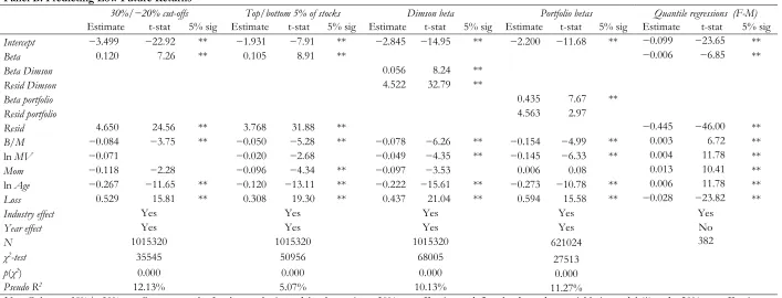
Our main tests in Table 4 use arbitrary cut-off points of 20% and −15% to define the dependent
variables in models (1) and (2). In sensitivity tests, we first check if our conclusions are robust to two
alternative definitions of the two dependent variables. First, we repeat the logit models using a 30%
cut-off point to define the dependent variable in model (1) and a −20% cut-off point to define the
15 stocks to the high return portfolio and 5.3% of stocks to the low return portfolio. This compares to
9.5% and 11% of stocks in the high and low return portfolio using the 20% and −15% breakpoints.
Second, each month we calculate the mean monthly return over the previous three months for each
stock. Then we calculate the mean return for the 5% of stocks with the highest previous
three-month returns. The dependent variable for model (1) takes the value of one if the stock’s mean
monthly return is higher than the mean return of stocks in the top vigintile formed based on the past
three-month returns, and is zero otherwise. We follow a similar procedure to define the dependent
variable for model (2), but now our cut-off point is based on the mean return for the 5% of stocks
with the lowest average returns calculated over the previous three months.22 The first columns of
Table 5 report the regression results for the two logit models when using the two alternative ways to
define the dependent variables. The coefficients on betas are positive and significant in both cases,
consistent with the results in Table 4. This suggests that the magnitude of the arbitrary cut-off points
has no effect on the validity of our inferences.
[Insert Table 5 here]
Other Beta Estimation Methods
Next, we consider the effect that the beta estimation method has on our inferences. Specifically, we
use Dimson’s (1979) beta to control for the thin trading bias in beta estimates, and portfolio betas to
test the sensitivity of our results to the errors-in-variables problem. The regression results for
Dimson beta and portfolio beta in Table 5 show positive and significant coefficients on betas in
models (1) and (2). This indicates that our inferences that beta reflects risk are not sensitive to the
16 Quantile Regressions
In our main tests we use two logit models because they offer a simple and robust way to test the risk
interpretation for beta and the models build directly on the intuition that high risk stocks should
cluster in the tails of the cross-sectional return distribution. Next we show that we reach similar
conclusions when we use non-parametric quantile regressions. Quantile models allow us to
investigate the relation between beta and returns for the top and bottom decile of the return
distribution. If beta reflects risk, beta should be a strong return predictor in the top and the bottom
return decile.
To implement quantile regressions, we set up two models, one explaining the top decile of
monthly stock returns (the high return portfolio) and the other explaining the bottom decile of
monthly stock returns (the low return portfolio). The specifications of the two models are:
90( ) 0 0 0 0
Q return Beta Controls u (4) Q return10( ) 1 1Beta 1Controls u 1 (5)
where the set of controls is the same as in models (1) and (2). For models (4) and (5), it is critical to
recognize that if beta reflects risk, beta coefficients in the two regressions should have opposite
signs. To clarify, if high betas indicate more risky stocks, then the coefficient on beta should be
positive in the regression explaining the top returns decile, θ0>0, i.e. high beta stocks should
associate with more positive returns in the right tail of the return distribution. However, for stocks
in the bottom return decile, the coefficient on beta should be negative, θ1<0, i.e. returns should be
decreasing in beta in the left tail of the return distribution.
Columns Quantile regressions (F-M) in Table 5 report the results for the two quantile regressions (4) and (5). Because quantile regressions do not allow for clustering of standard errors,
we use the Fama-MacBeth method to control (at minimum) for the time-series dependence of
17 explaining the top return decile, i.e. high beta stocks tend to have large positive returns in the right
tail of the return distribution. The coefficient on beta is negative in the regression for the bottom
return decile. This is in line with the prediction that high beta stocks should have more negative
returns in the left tail of the return distribution. Together, the quantile regression results support our
conclusion that beta captures risk.
Unreported additional results
In unreported results, we perform four further tests. First, we find that our conclusions from
Table 4 are unchanged when we use 12-month buy-and-hold returns and cut-off points of 75% to
define the dependent variable for model (1) and −50% for model (2).24 Second, our conclusions
from Table 4 are unchanged when we use a simultaneous regression model to jointly estimate
models (1) and (2), which allows for potential correlation in error terms between the two models.25
Third, we document positive and significant coefficients on betas in both logit models when we
repeat logit regressions (1) and (2) for each decade over our sample period. This shows that our
conclusion that beta predicts large positive and large negative returns are not driven by a specific
sample period. Fourth, we find that betas predict returns for other parts of the return distribution
than the tails. Specifically, each month we split stocks into quintiles based on their returns and use a
multinomial logistic regression to predict returns for each quintile portfolio. We find that beta
coefficients are significant in all regressions. Further, we confirm our earlier conclusion that the
relation between beta and returns is U-shaped. Specifically, the coefficients on betas reduce in
magnitude when moving from portfolios located in the left and right tail of the return distribution to
portfolios in the center of the return distribution. This is consistent with the intuition that stock risk
reduces moving from the tails to the center of the return distribution and corroborates our
18 CONCLUSIONS
Previous studies find no evidence of a significant cross-sectional relation between beta and returns,
which questions whether market risk helps explain the return cross-section. This study builds on the
intuition that risky stocks should concentrate in the tails of the cross-sectional return distribution to
test if stock returns reflect beta risk. Using two logistic regressions, one predicting large positive
returns and the other predicting large negative returns, we show that high beta stocks cluster in the
tails of the cross-sectional return distribution. This supports the prediction that high beta stocks are
more risky. Our results validate the use of market beta as a risk control in empirical accounting and
19 REFERENCES
Abarbanell J., and V. Bernard, ‘Is the U.S. Stock Market Myopic?’, Journal of Accounting Research, Vol. 38, 2000.
Amihud Y., B.J. Christensen and H. Mendelson, ‘Further Evidence on the Risk-Return Relationship’, Working paper, New York University, 1993.
Anderson J.A., and R.W. Faff, ‘Point and Figure Charting: A Computational Methodology and
Trading Rule Performance in the S&P 500 Futures Market’, International Review of Financial Analysis, Vol. 17, 2006.
Ané T., and H. Geman, ‘Order Flow, Transaction Clock, and Normality of Asset Returns’, Journal of Finance, Vol. 55, 2000.
Ball R., and P. Brown, ‘An Empirical Evaluation of Accounting Income Numbers’, Journal of Accounting Research, Vol. 6, 1968.
Benson, K., and R.W. Faff, ‘β’, Abacus, Vol. 49, 2013.
Berkman, H., ‘The Capital Asset Pricing Model: A Revolutionary Idea in Finance!’, Abacus, Vol. 49, 2013.
Bilinski P., and J. Ohlson, ‘Risk vs. Anomaly: A New Methodology Applied to ‘Accruals’’, Working paper, NYU Stern School of Business, 2012.
Black F., M. Jensen and M. Scholes, ‘The Capital Asset Pricing Model: Some Empirical Tests’, in M.
Jensen (ed.), Studies in the Theory of Capital Markets, Praeger, 1972.
Blume, M.E., and I. Friend, ‘A New Look at the Capital Asset Pricing Model’, Journal of Finance, Vol. 28, 1973.
Bornholt, G., ‘The Failure of the Capital Asset Pricing Model (CAPM): An Update and Discussion’,
20 Bos, T., and P. Newbold, ‘An Empirical Investigation of the Possibility of Stochastic Systematic Risk
in the Market Model’, Journal of Business, Vol. 57, 1984.
Brav, A., R. Lehavy and R. Michaely, ‘Using Expectations to Test Asset Pricing Models’, Financial Management, Vol. 34, 2005.
Cai, Ch.X., I. Clacher, and K. Keasey, ‘Consequences of the Capital Asset Pricing Model (CAPM)—
a Critical and Broad Perspective’, Abacus, Vol. 49, 2013.
Campbell, J., J. Hilscher and J. Szilagyi, ‘In Search of Distress Risk’, Journal of Finance, Vol. 63, 2008. Chan, K.C., and N. Chen, ‘Structural and Return Characteristics of Small and Large Firms’, Journal of
Finance, Vol. 46, 1991.
Chan, K.C., and J. Lakonishok, ‘Are the Reports of Beta’s Death Premature?’, Journal of Portfolio Management, Vol. 19, 1993.
Christensen, H., E. Lee and M. Walker, ‘Do IFRS Reconciliations Convey Information?, The effect
of debt contracting. Journal of Accounting Research, Vol. 47, 2009.
Chung, Y.P., H. Johnson and M.J. Schill, ‘Asset Pricing when Returns are Nonnormal: Fama‐French
Factors versus Higher‐Order Systematic Comoments’, Journal of Business, Vol. 79, 2006.
Coles, J., and U. Loewenstein, ‘Equilibrium pricing and portfolio composition in the presence of
uncertain parameters’, Journal of Financial Economics, Vol. 22, 1988.
Collins, D.W., ’SEC Product-Line Reporting and Market Efficiency’, Journal of Financial Economics, 2, 1975.
Collins, D.W., E.L. Maydew and I.S. Weiss, ‘Changes in the Value Relevance of Earnings and Book
Values over the Past Forty Years’, Journal of Accounting and Economics, Vol. 24, 1997.
21 Daniel, K., and S. Titman, ‘Market Reactions to Tangible and Intangible Information’, Journal of
Finance, Vol. 61, 2006.
Dechow, P., and I. Dichev, ‘The Quality Of Accruals and Earnings: The Role of Accrual Estimation
Errors’, The Accounting Review, Vol. 77, 2002.
Dechow, P., and W. Ge, ‘The Persistence of Earnings and Cash Flows and the Role of Special
Items: Implications for the Accrual Anomaly’, Review of Accounting Studies, Vol. 11, 2006.
Dempsey, M., ‘The Capital Asset Pricing Model (CAPM): The History of a Failed Revolutionary
Idea in Finance? ’, Abacus, Vol. 49, 2013a.
Dempsey, M., ‘The CAPM: A Case of Elegance is for Tailors? ’, Abacus, Vol. 49, 2013b.
Diamond, D.W., and R.E. Verrecchia, ‘Disclosure, Liquidity, and the Cost of Capital’, Journal of Finance, Vol. 66, 1991.
Dichev, I., ‘Is the Risk of Bankruptcy a Systematic Risk?’, Journal of Finance, Vol. 53, 1998.
Dimson, E., ‘Risk Measurement when Shares are Subject to Infrequent Trading’, Journal of Financial Economics, Vol. 7, 1979.
Dimson, E., and P.R. Marsh, ‘The Stability of UK Risk Measures and the Problem of Thin Trading’,
Journal of Finance, Vol. 38, 1983.
Faff, R.W., ‘A Multivariate Test of a Dual-Beta CAPM: Australian Evidence’, Financial Review, Vol. 36, 2001.
Fama, E.F., and K.R. French, ‘The Cross-Section of Expected Stock Returns’, Journal of Finance, Vol. 47, 1992.
Fama, E.F., and K.R. French, ‘Common Risk Factors in the Returns on Stocks and Bonds’, Journal of Financial Economics, Vol. 33, 1993.
22 Fama, E.F., and J. MacBeth, ‘Risk, Return and Equilibrium: Empirical Tests’, Journal of Political
Economy, Vol. 81, 1973.
Ferson, W.E., and R.A. Korajczyk, ‘Do Arbitrage Pricing Models Explain the Predictability of Stock
Returns?’, Journal of Business, Vol. 68, 1995.
Francis, J., R. LaFond, P. Olsson, and K. Schipper, ‘The Market Pricing of Accruals Quality’, Journal of Accounting and Economics, Vol. 39, 2005.
Fu, F., ‘Idiosyncratic risk and the cross-section of expected stock returns’, Journal of Financial Economics, Vol. 91, 2009.
George, T., and C.H. Hwang, ‘A Resolution of the Distress Risk and Leverage Puzzles in the Cross
Section of Stock Returns’, Journal of Financial Journal of Political Economy, Vol. 96, 2010.
Gertler, M., and S. Gilchrist, ‘Monetary Policy, Business Cycles, and the Behavior of Small
Manufacturing Firms’, Quarterly Journal of Political Economics, Vol. 109, 1994.
Gomes, J., L. Kogan and L. Zhang, ‘Equilibrium Cross-Section of Returns’, Journal of Political Economy, Vol. 111, 2003.
Gow, I., G. Ormazabal, and D. Taylor, ‘Correcting for Cross‐Sectional and Time‐Series
Dependence in Accounting Research’, TheAccounting Review, Vol. 85, 2010.
Howton, S.W., and D.R.. Peterson, ‘An Examination of Cross-Sectional Realized Stock Returns using a Varying-Risk Beta Model’, Financial Review, Vol. 33, 1998.
Jagannathan, R., and Z. Wang, ‘The Conditional CAPM and Cross-Section of Expected Returns’,
Journal of Finance, Vol. 51, 1996.
Johnstone, D.J., ‘The CAPM Debate and the Logic and Philosophy of Finance’, Abacus, Vol. 49,
2013.
Kim, D., ‘The errors in the Variables Problem in the Cross-Section of Expected Stock Returns’,
23 Kothari, S.P., and J. Shanken, ‘Book-to-Market, Dividend Yield, and Expected Market Returns: A
Time-Series Analysis’, Journal of Financial Economics, Vol. 44, 1997.
Kothari, S.P., J. Shanken and R.G. Sloan, ‘Another Look at the Cross-Section of Expected Stock
Returns’, Journal of Finance, Vol. 50, 1995.
Lakonishok, J., and A. Shapiro, ‘Systematic Risk, Total Risk and Size as Determinants of Stock
Market Returns’, Journal of Banking and Finance, Vol. 10, 1986. Lindley, D., ‘A Statistical Paradox’, Biometrica, Vol. 44, 1957.
Lintner, J., ‘The Valuation of Risk Assets and Selection of Risky Investments in Stock Portfolios and
Capital Budgets’, Review of Economics and Statistics, Vol. 47, 1965.
Lo, A., and C. MacKinlay, ‘Data-snooping Biases in Tests of Financial Asset Pricing Models’, Review of Financial Studies, Vol. 3, 1990.
McNichols, M., ‘Discussion of ‘‘The Quality of Accruals and Earnings: The Role of Accrual
Estimation Errors’’’, TheAccounting Review, Vol. 77, 2002.
Mech, T., ‘Portfolio Return Autocorrelation’, Journal of Financial Economics, Vol. 34, 1993.
Modigliani, F., and M. Miller, ‘The Cost of Capital, Corporation Finance, and the Theory of
Investment’, American Economic Review, Vol. 48, 1958.
Moosa, I.A., ‘The Capital Asset Pricing Model (CAPM): The History of a Failed Revolutionary Idea
in Finance?’ Comments and Extensions’, Abacus, Vol. 49, 2013.
Ohlson, J., ‘Financial Ratios and the Probabilistic Prediction of Bankruptcy’, Journal of Accounting Research, Vol. 19, 1980.
Partington, G., ‘Death Where is Thy Sting? A Response to Dempsey's Despatching of the CAPM’,
Abacus, Vol. 49, 2013.
24 Penman, S.H., ‘An Empirical Investigation of the Voluntary Disclosure of Corporate Earnings
Forecasts’, Journal of Accounting Research, Vol. 18, 1980.
Penman, S.H., ‘Financial Forecasting, Risk, and Valuation: Accounting for the Future’, Abacus, Vol. 46, 2010.
Penman, S.H., ‘Accounting for Risk and Return in Equity Valuation’, Journal of Applied Corporate Finance, Vol. 23, 2011.
Penman, S.H., and T. Sougiannis, ‘A Comparison of Dividend, Cash Flow, and Earnings
Approaches to Equity Valuation’, Contemporary Accounting Research, Vol. 15, 1998.
Perez-Quiros, G., and A. Timmermann, ‘Firm Size and Cyclical Variations in Stock Returns’, Journal of Finance, Vol. 55, 2000.
Pettengill G.N., S. Sundaram, and I. Mathur, ‘The Conditional Relation between Beta and Returns’,
The Journal of Financial and Quantitative Analysis, Vol. 30, 1995.
Ritter, J.R., and N. Chopra, ‘Portfolio Rebalancing and the Turn-Of-The-Year-Effect’, Journal of Finance, Vol. 44, 1989.
Roll, R., ‘A Critique of the Asset Pricing Theory’s Tests; Part I: On Past and Potential Testability of
the Theory’, Journal of Financial Economics, Vol. 4, 1977.
Sharpe, W.F., ‘Capital Asset Prices: A Theory of Market Equilibrium under Conditions of Risk’,
Journal of Finance, Vol. 19, 1964.
Shumway, T., ‘The Delisting Bias in CRSP Data’, Journal of Finance, Vol. 52, 1997.
Shumway, T., and V. Warther, ‘The Delisting Bias in CRSP's Nasdaq Data and its Implications for
the Size Effect’, Journal of Finance, Vol. 54, 1999.
Sloan, R., ‘Do stock prices fully reflect information in accruals and cash flows about future
25 Smith, T., and K. Walsh, ‘Why the CAPM is Half-Right and Everything Else is Wrong’, Abacus, Vol.
49, 2013.
Stambaugh, R.F., ‘On the Exclusion of Assets from Tests of the Two-Parameter Model: A
Sensitivity Analysis’, Journal of Financial Economics, Vol. 10, 1982.
Subrahmanyam, A., ‘Comments and Perspectives on ‘The Capital Asset Pricing Model’’, Abacus, Vol. 49, 2013.
Verrecchia, R., ‘Essays on Disclosure’, Journal of Accounting and Economics, Vol. 22, 97–180, 2001. Watts, R.L., and J.L. Zimmerman, ‘Positive Accounting Theory’, Prentice Hall, 1986.
26 TABLE 1
DESCRIPTIVE STATISTICS Panel A: Descriptive Statistics (N=1,015,320)
Mean Median STD Lower Quartile Upper Quartile
Return 1.6% 0.0% 17.1% −6.1% 7.4%
Beta 1.050 0.961 0.796 0.511 1.473
Resid 0.133 0.112 0.078 0.077 0.166
B/M 0.947 0.732 0.808 0.413 1.215
MV 1035.690 104.142 3206.760 24.185 523.552
Mom 3.7% −0.5% 36.4% −17.4% 18.1%
Age 15.661 10.756 14.186 5.918 19.923
Loss 24.1% 0.0% 42.8% 0.0% 0.0%
Panel B: Pearson Correlation Coefficients (N =1,015,320)
Return Beta Resid B/M MV Mom Age
Beta 0.003
p 0.011
Resid 0.011 0.366
p 0.000 0.000
B/M 0.031 −0.120 −0.060
p 0.000 0.000 0.000
MV −0.011 −0.022 −0.191 −0.162
p 0.000 0.000 0.000 0.000
Mom −0.001 0.094 0.114 −0.015 0.021
p 0.459 0.000 0.000 0.000 0.000
Age −0.007 −0.127 −0.322 0.014 0.360 −0.010
p 0.000 0.000 0.000 0.000 0.000 0.000
Loss 0.008 0.129 0.430 0.053 −0.117 −0.076 −0.144
p 0.000 0.000 0.000 0.000 0.000 0.000 0.000
27 TABLE 2
PORTFOLIO ANALYSIS Panel A: Mean Returns for Sorts on Beta
High beta Beta 2 Beta 3 Beta 4 Beta 5 Beta 6 Beta 7 Beta 8 Beta 9 Low beta High−Low
Beta 2.631 1.850 1.478 1.223 1.027 0.852 0.685 0.517 0.316 −0.076 2.707
Return 1.57% 1.53% 1.63% 1.60% 1.52% 1.59% 1.54% 1.57% 1.55% 1.59% −0.02%
Panel B: Mean Betas for Sorts on Returns
High return Return 2 Return 3 Return 4 Return 5 Return 6 Return 7 Return 8 Return 9 Low return High−Low Return 30.96% 12.28% 7.19% 4.05% 1.53% −0.71% −3.13% −6.00% −10.17% −20.83% 51.79%
Beta 1.206 1.086 0.999 0.948 0.924 0.924 0.962 1.033 1.138 1.284 −0.078
Panel C: Mean Betas for Portfolios Created on Double Sorts on Firm Size and Returns
High return Return 2 Return 3 Return 4 Return 5 Return 6 Return 7 Return 8 Return 9 Low return High−Low
Small 1.217 1.077 1.009 0.967 0.946 0.940 0.968 1.013 1.097 1.310 0.093
MV 2 1.317 1.137 1.036 0.980 0.958 0.965 0.989 1.060 1.207 1.415 0.098
MV 3 1.381 1.167 1.051 0.987 0.963 0.963 1.014 1.080 1.235 1.486 0.105
MV 4 1.390 1.154 1.068 1.004 0.989 0.980 1.038 1.124 1.261 1.482 0.092
MV 5 1.360 1.172 1.082 1.024 1.009 1.002 1.035 1.124 1.253 1.491 0.130
MV 6 1.339 1.159 1.064 1.006 0.988 0.975 1.009 1.104 1.226 1.432 0.093
MV 7 1.260 1.075 0.992 0.952 0.911 0.925 0.965 1.054 1.163 1.335 0.075
MV 8 1.186 1.044 0.931 0.881 0.857 0.867 0.919 0.996 1.102 1.269 0.084
MV 9 1.095 0.976 0.884 0.833 0.823 0.848 0.877 0.932 1.024 1.170 0.076
Large 0.912 0.821 0.743 0.733 0.690 0.695 0.738 0.796 0.837 0.950 0.038
28 TABLE 3
POOLED OLS AND FAMA-MACBETH REGRESSIONS OF MONTHLY STOCKS RETURNS ON MARKET BETA AND OTHER RISK CONTROLS
Regression 1 Regression 2 Regression 3 Portfolio betas Fama MacBeth Dimson beta Estimate t-stat 5% sig Estimate t-stat 5% sig Estimate t-stat 5% sig Estimate t-stat 5% sig Estimate t-stat 5% sig Estimate t-stat 5% sig Intercept 0.017 1.85 0.023 2.15 0.020 1.96 0.024 1.86 0.005 1.27 0.020 1.93
Beta 0.000 −0.15 0.001 0.53 0.001 0.62 0.000 0.10
Resid 0.003 0.12 0.004 0.17 0.023 1.72
Beta portfolio 0.005 0.93
Resid portfolio −0.251 −1.34
Beta dimson 0.000 0.46
Resid dimson 0.006 0.31
B/M 0.004 5.53 ** 0.004 5.42 ** 0.004 4.78 ** 0.003 4.73 ** 0.004 5.43 **
ln MV −0.002 −3.89 ** −0.002 −4.17 ** −0.002 −4.17 ** −0.002 −4.75 ** −0.002 −3.75 **
Mom 0.001 0.45 0.004 1.06 0.003 2.18 ** 0.001 0.45
ln Age 0.001 2.25 0.000 0.59 0.001 3.34 ** 0.001 2.10
Loss 0.000 0.08 0.002 0.68 −0.001 −0.54 0.000 0.07
Industry effect Yes Yes Yes Yes Yes Yes
Year effect Yes Yes Yes Yes No Yes
N 1015320 1015320 1015320 621024 382 1015320
F-test 144.52 150.95 141.95 146.57 142.21
p(F) 0.000 0.000 0.000 0.000 0.000
R2 0.47% 0.58% 0.58% 0.90% 0.58%
[image:29.842.81.768.114.385.2]29 TABLE 4
LOGISTIC REGRESSIONS PREDICTING HIGH AND LOW FUTURE RETURNS
Panel A: Predicting High Future Returns
Regression 1 Regression 2 Regression 3 Fama MacBeth
Estimate ME (%) t-stat 5% sig Estimate ME (%) t-stat 5% sig Estimate ME (%) t-stat 5% sig Estimate t-stat 5% sig
Intercept −2.830 −40.43 ** −2.659 −21.70 ** −2.377 −19.42 ** −4.832 −16.60 **
Beta 0.329 0.262 8.33 ** 0.173 0.138 8.24 ** 0.154 0.123 8.47 ** 0.128 6.78 **
Resid 3.604 0.283 27.68 ** 2.932 0.230 21.71 ** 3.122 8.83 **
B/M 0.014 0.012 0.76 0.022 0.018 1.29 −0.118 −1.55
ln MV −0.173 −0.370 −9.38 ** −0.143 −0.306 −7.89 ** −0.256 −21.06 **
Mom 0.004 0.002 0.15 0.014 0.31
ln Age −0.168 −0.124 −11.61 ** −0.158 −3.29 **
Loss 0.301 0.129 14.16 ** 0.236 3.87 **
Industry effect No Yes Yes Yes
Year effect No Yes Yes No
N 1015320 1015320 1015320 382
χ2-test 3739 31672 35123
p(χ2) 0.000 0.000 0.000
Pseudo R2 1.00% 6.87% 7.22%
30 TABLE 4 (continued)
Panel B: Predicting Low Future Returns
Regression 1 Regression 2 Regression 3 Fama MacBeth
Estimate ME (%) t-stat 5% sig Estimate ME (%) t-stat 5% sig Estimate ME (%) t-stat 5% sig Estimate t-stat 5% sig Intercept −2.719 −25.13 ** −3.156 −28.25 ** −2.874 −23.08 ** −3.997 −13.92 ** Beta 0.365 29.1% 7.98 ** 0.150 12.0% 8.29 ** 0.125 9.9% 7.70 ** 0.109 4.75 **
Resid 5.243 41.1% 24.92 ** 4.407 34.6% 24.91 ** 5.083 22.82 **
B/M −0.088 −7.2% −3.77 ** −0.076 −6.2% −3.75 ** −0.117 −2.79 **
ln MV −0.108 −23.0% −6.02 ** −0.062 −13.2% −4.06 ** −0.174 −15.20 **
Mom −0.095 −3.5% −2.29 −0.248 −4.57 **
ln Age −0.214 −15.9% −10.45 ** −0.276 −12.87 **
Loss 0.434 18.6% 17.20 ** 0.507 11.62 **
Industry effect No Yes Yes Yes
Year effect No Yes Yes No
N 1015320 1015320 1015320 382
χ2-test 3542 35479 41853
p(χ2) 0.000 0.000 0.000
Pseudo R2 1.28% 9.51% 10.23%
Note: Panel A presents the results for logit model (1) where the dependent variable, High_ret, is a dummy variable that takes the value of one if the stock’s monthly returns are higher than 20%, and is zero otherwise. Panel B reports results for logit model (2) where the dependent variable, Low_ret, is a dummy variable that takes the value of one if the stock’s monthly returns are lower than −15%, and is zero otherwise. Other variable definitions are in Table 1. Industry effect and Year effect are industry and year dummies. ME (%) shows the marginal effects in percentages. For the Fama MacBeth regressions, t-statistics are based on the time-series standard errors. For all other regressions, t- statistics are based on dual-clustered standard errors. 5% sig equals ** to indicate significance at the 5% level using sample size-adjusted critical values calculated as [(N−1)(N1/N−1)]0.5, where N is the
[image:31.842.74.783.105.335.2]31 TABLE 5
LOGIT MODELS PREDICTING HIGH AND LOW FUTURE RETURNS: SENSITIVITY ANALYSIS Panel A: Predicting High Future Returns
30%/−20% cut-offs Top/bottom 5% of stocks Dimson beta Portfolio betas Quantile regressions (F-M) Estimate t-stat 5% sig Estimate t-stat 5% sig Estimate t-stat 5% sig Estimate t-stat 5% sig Estimate t-stat 5% sig Intercept −2.966 −17.93 ** −1.760 −7.37 ** −2.363 −12.72 ** −2.048 −9.70 ** 0.118 17.32 **
Beta 0.144 6.58 ** 0.118 10.84 ** 0.006 4.14 **
Beta Dimson 0.065 9.66 **
Resid Dimson 3.163 26.00 **
Beta portfolio 0.504 7.49 **
Resid portfolio −1.243 −0.62
Resid 3.559 21.74 ** 2.191 19.43 ** 0.585 23.85 **
B/M 0.013 0.60 0.030 3.17 0.021 1.88 −0.013 −0.54 0.002 3.05 **
ln MV −0.224 −7.85 ** −0.036 −3.48 −0.127 −10.14 ** −0.196 −7.90 ** −0.007 −13.56 **
Mom −0.042 −1.18 0.042 1.92 0.000 0.01 0.127 2.91 −0.004 −1.91
ln Age −0.203 −12.99 ** −0.088 −9.58 ** −0.176 −14.58 ** −0.231 −13.11 ** −0.004 −5.30 ** Loss 0.477 16.28 ** 0.143 9.14 ** 0.304 16.69 ** 0.443 20.70 ** 0.030 14.49 **
Industry effect Yes Yes Yes Yes Yes
Year effect Yes Yes Yes Yes No
N 1015320 1015320 1015320 621024 382
χ2-test 31782 29602 46035 23729
p(χ2) 0.000 0.000 0.000 0.000
Pseudo R2 10.70% 3.01% 7.11% 8.13%
32 TABLE 5 (continued)
Panel B: Predicting Low Future Returns
30%/−20% cut-offs Top/bottom 5% of stocks Dimson beta Portfolio betas Quantile regressions (F-M) Estimate t-stat 5% sig Estimate t-stat 5% sig Estimate t-stat 5% sig Estimate t-stat 5% sig Estimate t-stat 5% sig Intercept −3.499 −22.92 ** −1.931 −7.91 ** −2.845 −14.95 ** −2.200 −11.68 ** −0.099 −23.65 **
Beta 0.120 7.26 ** 0.105 8.91 ** −0.006 −6.85 **
Beta Dimson 0.056 8.24 **
Resid Dimson 4.522 32.79 **
Beta portfolio 0.435 7.67 **
Resid portfolio 4.563 2.97
Resid 4.650 24.56 ** 3.768 31.88 ** −0.445 −46.00 **
B/M −0.084 −3.75 ** −0.050 −5.28 ** −0.078 −6.26 ** −0.154 −4.99 ** 0.003 6.72 ** ln MV −0.071 −0.020 −2.68 −0.049 −4.35 ** −0.145 −6.33 ** 0.004 11.78 ** Mom −0.118 −2.28 −0.096 −4.34 ** −0.097 −3.53 0.006 0.08 0.013 10.41 ** ln Age −0.267 −11.65 ** −0.120 −13.11 ** −0.222 −15.61 ** −0.273 −10.78 ** 0.006 11.78 ** Loss 0.529 15.81 ** 0.308 19.30 ** 0.437 21.04 ** 0.594 15.58 ** −0.028 −23.82 **
Industry effect Yes Yes Yes Yes Yes
Year effect Yes Yes Yes Yes No
N 1015320 1015320 1015320 621024 382
χ2-test 35545 50956 68005
27513
p(χ2) 0.000 0.000 0.000 0.000
Pseudo R2 12.13% 5.07% 10.13% 11.27%
Note: Columns 30%/−20% cut-offs report results for the two logit models when using a 30% cut-off point to define the dependent variable in model (1) and −20% cut-off point to define the dependent variable in model (2). Columns Top/bottom 5% of stocks present results where the dependent variable for model (1) takes the value of one if the stock’s monthly return is higher than the mean return of stocks in the top vigintile formed on the past three-month returns, and is zero otherwise. We follow a similar procedure to define the dependent variable for model (2), but now our cut-off point is based on mean returns for the 5% of stocks with the lowest average returns calculated over the previous three months. Columns Dimson beta report results when we use Dimson’s (1979) beta in models (1) and (2). Columns Portfolio betas present results when using portfolio betas. Columns Quantile regressions (F-M) report Fama-MacBeth quantile regressions for the top and bottom return deciles. See Table 1 for other variable definitions. Industry effect and Year effect are industry and year dummies. For Quantile regressions (F-M), the t-statistics are based on time-clustered standard errors. For all other regressions, the t- statistics are based on dual-clustered standard errors. 5% sig equals ** to indicate significance at the 5% level using sample size-adjusted critical values calculated as [(N−1)(N1/N−1)]0.5, where N is the number
of observations.
[image:33.842.74.781.104.374.2]33
1 The CAPM’s beta is commonly used to compute the cost of capital, which is applied to capital budgeting problems
or in valuation (Penman and Sougiannis, 1998; Abarbanell and Bernard, 2000). The CAPM is also used to evaluate
the information content of public disclosure (Ball and Brown, 1968; Penman, 1980), fund managers performance
(Pastor and Stambaugh, 2002), and of new regulation (Collins, 1975, Christensen et al., 2009). The importance of market beta in accounting and finance research is emphasized in Benson and Faff (2013), Berkman (2013), Bornholt
et al. (2013), Cai et al. (2013), Johnstone (2013), Dempsey (2013a, 2013b), Moosa (2013), Partington (2013), Smith and Walsh (2013) and Subrahmanyam (2013).
2 To explain beta’s failure to describe the return cross-section, studies identified shortcomings in empirical CAPM
tests that could explain its poor performance. Roll (1977) argues that the market portfolio in the CAPM is
unobserved and that empirical tests that use the stock market index to approximate the market portfolio do not
provide valid CAPM tests. However, Stambaugh (1982) shows that tests of the CAPM are insensitive to the
specification of the market benchmark. Chan and Lakonishok (1993) argue that noise in the return data limits the
ability of empirical tests to conclude on the positive relation between beta and returns. Later studies focused on the
empirical issues related to using realized rather than expected returns in CAPM tests (Brav et al., 2005), the errors-in-variables problem (Kim, 1995), and the time-variation in asset risk premia (Jagannathan and Wang, 1996; Ferson and
Korajczyk, 1995).
3 Misspecification of the asset pricing model leads to incorrect discount rate estimates and consequently stock
misvaluation. In event studies, it can lead to erroneous conclusions on the existence of abnormal stock returns and
market inefficiencies where none exist. Finally, a strong correlation between beta and various accounting measures,
e.g. between beta and accruals (Francis et al., 2005), can produce significant coefficients on the accounting measures in pricing tests when beta is omitted from the return regression (omitted variable bias).
4 This intuition links directly with the CAPM theory that high beta stocks earn higher expected returns as a
compensation for high systematic risk, i.e. higher likelihood that ex-post outcomes will strongly deviate from
expected outcomes.
5 We use asymmetric cut-off points to define the dependent variables for the logit regressions to adjust for the fact
that the distribution of returns is right-skewed.
6 Our main tests are implemented ex-post as we need to know future returns to identify stocks with large positive
and negative returns. We do not see this as a disadvantage as (1) we do not claim to test viable trading strategies, (2)
ex-post tests are common in empirical accounting research (e.g. estimates of earnings persistence in Dechow and
Ge, 2006 and current accruals in Dechow and Dichev, 2002 and McNichols, 2002) and (3) robustness tests show
that our conclusions are unaffected when we specify the dependent variables in the two logit models based on past