The approximate determinantal assignment problem

(1)

City, University of London Institutional Repository

Citation:

Petroulakis, G. (2015). The approximate determinantal assignment problem. (Unpublished Doctoral thesis, City University London)

This is the accepted version of the paper.

This version of the publication may differ from the final published

version.

Permanent repository link:

http://openaccess.city.ac.uk/11894/

Link to published version:

Copyright and reuse: City Research Online aims to make research

outputs of City, University of London available to a wider audience.

Copyright and Moral Rights remain with the author(s) and/or copyright

holders. URLs from City Research Online may be freely distributed and

linked to.

City Research Online: http://openaccess.city.ac.uk/ [email protected]

(2)

THE APPROXIMATE

DETERMINANTAL ASSIGNMENT

PROBLEM

George Petroulakis

A thesis submitted for the degree of Doctor

of Philosophy

City University London, School of

Mathematics, Computer Science and

Engineering, EC1V OHB, London, United

Kingdom

(3)

Acknowledgements

I would like to acknowledge the help of various people who contributed in one way or another during my research.

My gratitude goes, first and foremost, to my supervisors Professor N. Karca-nias and Dr. J. Leventides. Prof. KarcaKarca-nias has introduced me to one of the most exciting fields in Mathematics, the Algebraic Control Theory that combines techniques and results from a wide variety of mathematical areas, as well as other scientific fields. His ideas were fluent and we are still working on some of them.

I am also particularly grateful to Dr. Leventides for his invaluable help. His personal work on the 2-dimensional case of the problem gave me the right foun-dations to connect the problem with new techniques (numerical algebraic geom-etry, Newton’s algorithm on manifolds, etc.) in low dimensions and evolve it via tensor theory in higher dimensions, which resulted in a series of promising and important results.

I would also like to thank Professor G. Halikias for the fruitful discussions on the SVD and the stability radii and Professor B. Sturmfels for his help on how to execute the Macaulay 2 software, in order to verify some of my outcomes.

(7)

Abstract

The Determinantal Assignment Problem (DAP) is one of the central problems of Algebraic Control Theory and refers to solving a system of non-linear algebraic equations to place the critical frequencies of the system to specified locations. This problem is decomposed into a linear and a multi-linear subproblem and the solvability of the problem is reduced to an intersection of a linear variety with the Grassmann variety. The linear subproblem can be solved with standard methods of linear algebra, whereas the intersection problem is a problem within the area of algebraic geometry. One of the methods to deal with this problem is to solve the linear problem and then find which element of this linear space is closer -in terms of a metric - to the Grassmann variety. If the distance is zero then a solution for the intersection problem is found, otherwise we get an approximate solution for the problem, which is referred to as the approximate DAP.

In this thesis we examine the second case by introducing a number of new tools for the calculation of the minimum distance of a given parametrized multi-vector that describes the linear variety implied by the linear subproblem, from the Grass-mann variety as well as the decomposable vector that realizes this least distance, using constrained optimization techniques and other alternative methods, such as the SVD properties of the so called Grassmann matrix, polar decompositions and other tools. Furthermore, we give a number of new conditions for the appropri-ate nature of the approximappropri-ate polynomials which are implied by the approximappropri-ate solutions based on stability radius results.

(8)

Nonemclature

F: denotes a general field or ring, e.g., _R,_C.

a: denotes a scalar in F.

Fn_: _{denotes an}_n _{dimensional vector space over} _F_.

V: denotes an ordinary vector space or a vector space/set equipped with a special structure, e.g., varieties, manifolds, etc.

Vk

(V): denotes the k-th exterior power of a vector space V.

x: denotes a vector or ak-vector (multivector) onV orV1×· · ·×Vk,

respectively.

a∧b: denotes the wedge product (exterior product) between two k -vectors in Vk

(V).

R(s): denotes the field of rational functions.

F[s]: denotes the ring of polynomials over F.

I: denotes an ideal ofF[s].

Qm,n: denotes the set of lexicographically ordered, strictly increasing

sequences of m integers from 1,2,...,n.

Fm×n_: _{denotes the set of} _m_×_n _{matrices with elements from} _F_{, e.g.,}

Rm×n are all the real m×n matrices.

A: denotes a matrix in Fm×n

Nr(A),N`(A): denote the right and the left null space of a matrix A.

Ck(A): denotes thekth compound matrix of A∈ Fm×n, k ≤ {m, n}.

A⊗B: denotes the Kronecker product between two matricesAand B.

(9)

e₁⊗ · · · ⊗e_n: denotes the tensor product of the vectors e_i that belong to the vector spaces Vi, respectively, for i= 1, ..., n.

T: denotes a tensor/multi-dimensional array in V1 ⊗ · · · ⊗ Vn, for

the vector spaces Vi, i= 1, ..., n.

Pn(F): denotes the n-dimensional projective space for the field F.

Gr(m, V): denotes the set of allm-dimensional subspaces of ann-dimensional vector space V, called the Grassmannian.

Gm(V) or Gm,n: denotes the Grassmann variety of the projective space, implied

by the embedding ofGr(m, V) into the projective space_P(Vm

(V)).

MIMO: Multiple inputs-Multiple outputs.

DAP: Determinantal Assignment Problem.

QPR: Quadratic Pl¨ucker Relations.

CPD: CANDECOMP/PARAFAC Decomposition (Canonical Decom-position/Parallel Factors).

(10)

Chapter 1 Introduction

Control methodologies are central in the development of engineering design solutions to modern challenging applications. Control Technology is supported by a systems framework, where the study of system properties and the development of solutions to well defined problems are crucial. Control theory provides the backbone of control synthesis methods and control system design. It’s main aspects are:

i) Study of systems properties.

ii) Characterization of solvability conditions of exact control problems.

iii) Synthesis methods for control problems.

iv) Design methods.

These aspects are central to the development of design strategies and method-ologies since they provide the tools of analysis, formulation of objectives and development of control design approaches and methodologies. Control theory is model dependent and the richest part of it is that dealing with linear, time-invariant, finite dimensional (lumped parameter) systems. Such simple models seem to be appropriate for the Early Design stages where there is neither the scope nor the possibility for detailed modeling.

(11)

on the shaping of performance indicators usually following iterative approaches and they aim to satisfy system properties in an way to satisfy overall design objectives. Bridging the gap between synthesis and design methods involves the development of synthesis methods to a set up where model uncertainty is handled appropriately and approximate solutions to exact synthesis problems is derived, when exact solutions do not exist. This is a very valuable task since it will lead to the development of more powerful design methodologies relying on a combined shaping of performance indicators, handling model uncertainty and optimization based methods for deriving approximate solutions to exact problems.

Amongst the important synthesis methods are those referred to pole assignment, zero assignment, stabilization, etc., under a variety of static or dynamic, central-ized or decentralcentral-ized compensation schemes. Integral part to such methods is the characterization of solvability conditions in term of properties amongst the system invariants and the development of algorithms that provide solution to exact design problems. A major challenge in the development of effective design methodologies is the development of approximate solutions to exact synthesis problems. The need for such developments arises due to issues of model uncer-tainty, as well as investigating approximate solutions when the exact problems do not have a feasible solution from the engineering viewpoint (when solutions to the exact problems are complex or when there is uncertainty on the realistic values for the design objectives). This thesis aims to extend the potential of frequency assignment synthesis methods by enabling the development of approximate solu-tions to exact algebraic problems by formulating them as optimization problems that may be tackled by powerful numerical methods.

(12)

approx-imate solutions and further empower it with potential for studying stabilization problems. The importance of algebraic geometry for control theory problems has been demonstrated by the work in [Bro. & Byr. 2], [Mart. & Her. 1], etc. The approach adopted in [Gia. & Kar. 3], [Kar. & Gia. 5], [Kar. & Gia. 6], differs from that in [Bro. & Byr. 2], [Byr. 1] in the sense that the problem is stud-ied in a projective, rather than an affine space setting and contrary to that of [Bro. & Byr. 2], [Byr. 1] it can provide a computational approach. The DAP approach relies on exterior algebra, [Mar. 1] and on the explicit description of the Grassmann variety [Hod. & Ped. 1], in terms of the QPR, has the advantage of being computational, and allows the formulation of distance problems, which are required to turn the synthesis method to a design methodology.

The multilinear nature of DAP suggests that the natural framework for its study is that of exterior algebra [Mar. 1]. DAP [Kar. & Gia. 5] may be reduced to a linear problem of zero assignment of polynomial combinants and a standard problem of multi-linear algebra, the decomposability of multivectors [Mar. 1]. The solution of the linear subproblem, whenever it exists, defines a linear space in a projective space of the form_P(mn)−1 for n ≥ m, whereas decomposability is

characterized by the set of Quadratic Pl¨ucker Relations (QPR), which define the Grassmann variety of _P(mn)−1 [Hod. & Ped. 1]. Thus, the solvability of DAP is

reduced to a problem of finding real intersections between the linear variety and the Grassmann variety of the projective space. This Exterior Algebra-Algebraic Geometry method, has provided new invariants (Pl¨ucker Matrices and the Grass-mann vectors) for the characterization of rational vector spaces, solvability of control problems, ability to discuss both generic and non-generic cases and it is flexible as far as handling dynamic schemes, as well as structurally constrained compensation schemes. The additional advantage of the new framework is that it provides a unifying computational framework for finding the solutions, when such solutions exist. The multilinear nature of DAP has been handled by a “blow up” type methodology, using the notion of degenerate solution and known as “Global Linearisation” [Lev. 1], [Lev. & Kar. 3]. Under certain conditions, this method-ology allows the computation of solutions of the DAP problem.

The Determinantal Assignment Problem (DAP) has been crucial in unifying fam-ilies of frequency assignment as well as stabilization problems which underpin the development of a large number of algebraic synthesis problems but has also led to the introduction of many new challenges and problems of mathematical nature. Amongst these problems we distinguish:

(i) the development of methods for defining real intersections between varieties, a problem linked to realizability of solution in an engineering sense;

(13)

but also in the context of concrete problems (engineering problems are defined on concrete models);

(iii) computation of solutions to intersection problems (existence of intersections is only part of the problem);

(iv) handling issues of model uncertainty which requires the study of approx-imate solutions of DAP. The development of criteria for real intersections has been handled by developing cohomology algebra tools [Lev. & Kar. 2].

The issues linked to computation of solutions has led to the development of the Global Linearisation framework [Lev. 1], [Lev. & Kar. 3], which together with the set of Grassmann Invariants [Kar. & Gia. 5] provide the means for addressing problems defined on given models, as well as computing solutions. This frame-work is by no means completely developed and challenging problems exist such as overcoming difficulties of sensitivity of the Global Linearisation framework and extending it to the case where the models are characterized by uncertainty. The sensitivity issues may be handled by using Homotopy based methodologies [Chow., etc. 1] and by embedding the overall problem into the framework of con-strained optimization.

The model uncertainty issues opens up a new area where distance problems such as computing the distance of:

(i) a point from the Grassmann variety;

(ii) a linear variety from the Grassman variety;

(iii) parameterized families of linear varieties from the Grassmann variety;

(iv) relating the latter distance problems with properties of the stability domain [Bar. 1].

The study of these problems relate to classical problems such as spectral analy-sis of tensors, homotopy methods, constrained optimization, theory of algebraic invariants etc. This thesis addresses the development of DAP along the lines men-tioned above, and deals with a number of related mathematical problems which are crucial for the development of control problem solutions. The thesis has an in-terdisciplinary nature since it is in boundaries between Control and Mathematics. Control Theory defines the problems and the background concepts, Mathematics provides the solutions to well formulated problems and control Engineering deals with the implementation of the solutions of the mathematical problems and the development of algorithms and design methodology.

(14)

projective space and aims to introduce an analytic dimension by developing dis-tance problems and optimization tools. Thus, the novelty of this thesis is that it proposes the development of approximate solutions to purely algebraic problems and thus expand the potential of the existing algebraic framework by develop-ing its analytic dimension. The development of the ”approximate” dimension of DAP involves the study of a number of problems that can transform the existence results and general computational schemes to tools for control design. There are many challenging issues in the development of the DAP framework and amongst them are its ability to provide solutions even for non-generic cases, handle prob-lems of model uncertainty, as well as providing approximate solutions to the cases where generically there is no solution of the exact problem. The development of the approximate DAP requires a framework for approximation (provided by dis-tance problems) and the formulation of an appropriate constrained optimization problem.

Objectives: The objectives of this thesis are:

(i) To develop tools for the computation of the distance between the Grass-mann variety and point and a linear variety and the GrassGrass-mann variety of a Projective space, and find approximate solutions of Exterior equations.

(ii) To develop an integrated framework for approximate solutions of DAP and its extension to the case of stabilization problems.

(iii) To develop suitable algorithms that could provide the desirable approximate solutions in higher Grassmann-variety dimensions where tensors are used instead of matrices.

Our research has three aspects which are interlinked and are essential for the development and computation of approximate solutions of DAP. The first is the development of the approximate solutions of exterior equations and the study of all related mathematical problems. The second deals with the development of stability methodologies for general constrained Optimization Problems and finally its application to DAP. The first two are purely mathematical tasks and the last involves their integration to produce solutions to problems of control theory and control design which requires a combination of the two early parts together with control theoretic results to produce a methodology for robust approximate solutions to algebraic synthesis control problems. The main Activity area in which we will work is the area of Approximate Solutions of Exterior Equations and Distance Problems: The solution of exterior equations is an integral part of the DAP methodology, since it defines the multi-linear part of the problem. The problem of decomposability of a multivector z ∈ Vm

(U), where U is an

m-dimensional vector space of _Rn, is equivalent to the solvability of the exterior equation

(15)

Note that versions of such equations may be considered, where v_i and z vec-tors are polynomial vecvec-tors (the latter corresponds to dynamic versions of DAP [Lev. & Kar. 4]). The solvability of such equations is referred to as decompos-ability of the multi-vector z and are given by the set of quadratics which are known as the Quadratic Pl¨ucker Relations (QPRs) [Hod. & Ped. 1] of the space, or of the equivalent projective space _P† and they characterize the Grassmann variety G(m, n) or Gm(Rn) of P(

n

m)−1, [Hod. & Ped. 1]. Whenever a solution to

(1.1) exists, this is a vector space Vz = sp{vi}, i = 1, ..., m and for the control

problems defines the corresponding compensator. The overall solution of DAP is reduced to finding common solutions of (1.1) and of a linear equation P z = a, where a is a given vector characterizing the assigned polynomial and P an in-variant matrix of the given problem (existence of real intersections of the two varieties). Model uncertainty, or non-existence of a solution of (1.1) requires the definition and solution of appropriate problems, which are essential parts in the development of the DAP framework. The expected results will provide the math-ematical concepts and tools to develop the new approximate framework for DAP and the research is of pure mathematical nature.

The development of solutions to the research challenges defined before requires addressing specific problems and undertaking research by adopting appropriate methodology which is described below. The overall research is organized in work areas as described below:

(1) Approximate Decomposability Problem (ADP): Assume that for a given vector z ∈ _P(mn)−1, equation (1.1) does not have solution. Define a

vec-tor ˆz ∈ _P(mn)−1 with the least distance from z, which is decomposable, or

equivalently define the distance of z from the corresponding Grassmann variety.

(2) Variety Distance Problem (VDP): Given a vector ˆz ∈ _P(mn)−1 and a linear

variety K := K(a), a ∈ _Rn _of

P(

n

m)−1 defined by the solution of P z = a,

define the distance of K from the corresponding Grassmann variety.

(3) Approximate Intersection Problem (AIP): Given a vector ˆz ∈ _P(mn)−1 and

a linear variety K := K(a), a ∈ _Rn _of

P(

n

m)−1 defined by the solution of P z = a, define a vector ˆat ∈ _Rn _{such that the linear variety intersects}

with the Grassmann variety and the following conditions hold true: (i) ˆat

has minimum distance has minimum distance from a ; (ii) ˆat has minimum distance from a and corresponds to a stable polynomial.

(16)

[Kar. & Lev. 9]. This approach is based on the characterization of decompos-ability by the properties of a new family of matrices known as Grassmann Ma-trices [Kar. & Gia. 6] which has been introduced as an alternative criterion to the standard description of the Grassmann variety provided by the QPRs. This new approach handles simultaneously the question of decomposability and the reconstruction of Vz. For every z ∈

Vm

(U) with coordinates aω, ω ∈ Qm,n,

the Grassmann matrix Φm_n(z) of z is defined. In fact it has been shown, that rankΦm

n(z)≥n−m for all z 6= 0 and that z is decomposable, if and only if, the

equality sign holds. If rankΦm

n(z) = n−m then it was shown that the solution

spaceVz is defined byVz =Nr(Φmn(z)). The rank based test for decomposability

is easier to handle than the QPRs and provides a simple method for the compu-tation ofVz. The new test provides an alternative formulation for investigation of

existence, as well as computation of real solutions of DAP (R-DAP). Solvability of R-DAP is thus reduced to finding a vector such that the rank condition is satisfied.

The study of the above distance problem may be formulated as distance of a Grassmann matrix from the variety of matrices having certain rank and can be studied using approaches such as structural singular values. The characteriza-tion of the element with the least distance are the tasks here. This problem is also referred as approximate decomposability and it is a very difficult problem of multi-linear algebra that is not completely solved [Bad. & Kol. 1], [Dela., etc. 1]. In its general form, it is related to several important problems of multi-linear al-gebra, such as:

(a) Low rank tensor approximation;

(b) Multi-linear singular value decomposition;

(c) Determination of the tensor rank.

The main theme of these problems is to decompose a tensorT as a sum of rank one tensors, i.e., a sum of decomposable tensors. For the purposes of our work we will consider skew symmetric tensors, i.e, multi-linear tensorsT that arise from determinantal problems and we will try to approximate them by decomposable multi-vectors, i.e., to find vectorsa₁, ..., a_r such that the normkT−a₁∧ · · · ∧a_rk

(17)

In this thesis we will focus on providing a new means for computing approximate solutions for determinantal-type of problems,without the use of any generic (i.e., for almost all dynamical systems) or exact solvability conditions and algorithms which are based on them. Note that at first, the genericity problem was thought to be negligible in the sense that it lies in a union of algebraic subsets of lower dimension, [Her. & Mar. 1]. But several authors, e.g., [Ki. 1], [Caro., etc. 1], [Yan. & Ti. 1], [Ki. 2] have showed that under generic pole-assignable condi-tions, several essential control engineering attributes, e.g., sensitivity, stabil-ity, etc., may be lost. The algorithms that were presented for the solution of determinantal-type problems, mostly for the output feedback pole placement problem, [Rav., etc. 2], [Wan. & Ros. 2], [Ki., etc. 2] as well as the approach in [Sot. 1], [Sot. 2] have the same drawback; they are based on Kimuras generic pole assignability conditionm+p > n for an m-input,p-output, n-state MIMO system. The algorithms presented in this thesis may provide approximate solu-tions in any case, independently of generic or exact solvability condisolu-tions.

Our work is based on the observation that

(a multivector/matrix/tensor belongs to the Grassmann variety)⇔

(the multivector/matrix/tensor satisfies the QPR)⇔

(the multivector/matrix/tensor is decomposable)⇔

(the multivector/matrix/tensor has rank-1)

The first two equivalences have been well-examined in [Hod. & Ped. 1] and they are considered classic within the context of Algebraic Geometry. A number of some more recent results regarding the different forms these may take is met in [Gee. 1]. The last equivalence, with respect to the rank approach of a multivector, is mostly met in tensor theory; in the simplest case of matrices, a matrix A is said to have rank one if there exist vectors a, bsuch that

A=a×bt (1.2)

Consequently, the well-known rank ofA(the minimum number of column vectors needed to span the range of the matrix) is the length of the smallest decomposition of A into a sum of such rank-1 outer products, i.e.,

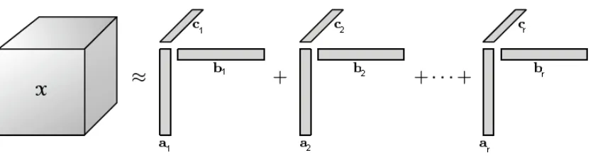
A=a₁×bt₁+· · ·+a_n×bt_n (1.3) In higher dimensions, matrix A is represented by a tensor and the above sum is referred to ashigher-order tensor decomposition, i.e.,

A =

r

X

i=1

Ai (1.4)

where Ai are rank one/decomposable tensors. If the matrix A in the sum (1.3)

(18)

best rank-one/decomposable approximation and this term is the best approximate solution ˆz of the determinantal assignment problem written as P z = a, when z

is decomposable that we mentioned before. For higher dimensions, the sum (1.4) can not guarantee which term is as closest to tensor A, [Kol. & Bad. 3], but at least we may achieve one decomposable approximation if A is a skew-symmetric tensor. In both cases the approximate solution yields an approximate polynomial ˆ

a(s) such that Pˆz = ˆa. We will study the stability properties of ˆa(s) with re-spect to the approximation ˆz and stability radius results and we will derive a new criterion for the stability of the approximate solution of DAP. Moreover, these results will be connected with the Grassmann matrix and alternative simplified formulae will be derived, which are completely new for best approximation prob-lems of this form.

For all the 2-dimensional Grassmann varieties, the Approximate Determinantal Assignment problem is completely solved as a manifold constrained optimization problem, where the derivation of the decomposable vector that best approximates the original controller, is based on eigenvalue decompositions (EVD), singular value decompositions or its generalizations, e.g., compact SVD, [Edel., etc. 1] or combinations of them. We present how these methods are expanded in or-der to yield parameterized approximate solutions in the projective space which is the natural space to examine a problem such as DAP. Uniqueness and non-uniqueness (degeneracy) issues of the decompositions that may arise are also examined in detail. Furthermore, we investigate how the approximate DAP is expanded into constrained minimization over more general varieties than the original ones (Generalized Grassmann varieties) and we derive a new Cauchy-Schwartz type inequality that provides a closed-form non-algorithmic solutions to a wide family of optimization problems related to best decomposable/ rank-1 problems. We provide a new criterion, to test the acceptability of the new approximate solution, i.e., whether the approximation lies in the stability do-main of the initial polynomial or not, by using stability radii theory. All results are compared with the ones that already exist in the respective literature (least squares approximations, convex optimization techniques, etc.), as well as with the results obtained by Algebraic Geometry Toolboxes, e.g., Macaulay 2. For numerical implementations, we examine under which conditions certain manifold constrained algorithms, such as Newton’s method for optimization on manifolds, could be adopted to DAP and we present a new algorithm which is ideal for DAP approximations.

(19)

involve non-uniqueness issues, several degenerate cases of higher order decom-positions may occur for the numeric CANDECOMP/PARAFAC decomposition, due to the fact that the rank of a tensor is not uniquely defined, as in the case of a matrix. This is also the reason that the method does not always guarantee that the approximation implied is actually the “best”, but it may be in any caseone decomposable approximation of the nominal tensor. These problems are much more complicated than the two dimensional case and only special cases of ten-sors have been examined so far, [Kol. & Bad. 3], [Raj. & Com. 1] regarding their non-uniqueness properties. The parametric decomposition of 3rd- order tensors is among the most important results of this thesis, since all tensor decompositions in the literature work for numerical data exclusively.

More analytically, in Chapter 2, we provide some of the control related math-ematical tools and notions. We present several descriptions of linear systems followed by the respective algebraic control theory background. We also discuss some aspects of general feedback configuration and we present the definition of the determinantal assignment problem (DAP) as the unifying problem of all fre-quency assignment-type problems.

In Chapter 3 we present all the mathematical tools that we are going to use through out this thesis. The purpose of this chapter is to clarify in simple terms, whenever this is possible, all the key mathematical tools that lie behind DAP and the several forms it may take. We begin with the basic concepts of multilinear algebra in order to construct the special space in which determinants are defined and examined, the so-called k-th exterior power implied by an ordinary vector space. This special space is obtained via the properties of the Exterior (or Grass-mann) Algebra which is a sub-algebra of the Tensor Algebra. We elaborate on the construction of these sets, since the basic frame of this thesis is based on the concept of tensors and we explain how a tensor/ multi-dimensional array is con-structed step-by-step by the vectors of the corresponding vector space. Finally, we present some basic notions and results regarding real affine and projective varieties, in order to define the Grassmann variety, a set whose several proper-ties and equivalent expressions are going to be used excessively in the following chapters.

(20)

the former category, we provide a purely numeric procedure, a full rank algo-rithm which was built for the output feedback problem where with some simple modifications it is adopted to DAP. However, owing to the nonlinear nature of the problem, the algorithm cannot be guaranteed in all cases to converge to a solution, [Pa. 1]. From the geometric techniques we refer to the Schubert calcu-lus methodology, the global linearization method, [Lev. 1], [Lev. & Kar. 3] and finally to the projective methodologies, [Fal. 1], [Gia. 1], [Kar. & Gia. 5] from which we will introduce the approximate DAP.

In Chapter 5, we interpret the approximate DAP, as a distance problem form the corresponding Grassmann variety for the 2-dimensional and its Hodge-dual case. We start from the simplest Grassmann variety which is described by one QPR only, in order to observe that the least distance from this variety is related to the singular values of a special matrix, the Grassmann matrix, [Kar. & Gia. 6]. The optimization problem is solved via the method of the Lagrange multipliers. We see, that this method can not be easily expanded to the higher dimensions due to the randomly increasing number of the QPR. We then derive a very important formula for 2-vector/2-skew symmetric tensor decomposition, the so calledprime decomposition where a 2-vector is written as a sum of decomposable vectors, one of which is its “best” approximation, i.e., the one in the Grassmann variety that achieves the least distance. The problem is studied at first via the Euclidean norm and then in the corresponding projective space via the gap metric.

(21)

In Chapter 7 we present how the problem of deriving the best decomposable/rank-1 approximation of a multivector for the 2-dimensional case, is actually a special case of the least distance problem between the multivector and the Generalized Grassmann varieties, a set that expands the notion of decomposability of the standard Grassmann variety, i.e., for a 2-vector a, a∧a = 0 corresponds to a decomposable/rank-1 vector, a∧a∧a= 0 to a sum of 2 decomposable vectors,

a∧a∧a∧a = 0 to a sum of 3 decomposable vectors, etc. This kind of gen-eralizations are very common within the area of linear-multilinear algebra due to the remarkable applications they may offer; a first generalization along with some useful computational analysis applications is observed in [Gol. & Van. 2], where a best-low rank matrix approximation was achieved for a matrix whose specified columns remained fixed. A generalization for low matrix-rank approxi-mation was also used in [Lu-S., etc. 1] for the design of two dimensional digital fil-ters, whereas several low-rank approximation generalizations of the Eckart-Young theorem, [Eck. & You. 1] were discussed in [Fri. & Tor. 1] and [Kol. 2], among others. Another generalization related to the Grassmann variety is presented in [Rav., etc. 1] via the use of the so called generalized Pl¨ucker embedding which was introduced for applications on dynamic output feedback problems. A differ-ent but well-known approach views the generalization of the Grassmann variety as the standard Grassmann variety which is preserved under any endomorphism from a vector space to itself, [Kolh. 1]. Nevertheless, this approach is only use-ful within the context of Lie algebra, which studies these varieties in relation with other algebraic objects, such as the Schur-S polynomials, rings, etc, and not for calculating best approximate solutions on hyper-sets, as in our case. Our approach lies in the concept of expanding the standard exterior algebra/tensor theories, [Hod. & Ped. 1], [Mar. 1] which is also met in the construction of the so-called generalized Grassmann algebras, where the properties of the classic ex-terior (Grassmann) algebra are equipped with multi-linear structures instead of bilinear ones, [Ohn. & Kam. 1], [Kwa. 1]. The most important result however of this chapter is the derivation of a new Cauchy-Schwartz type inequality which is suitable for solving these generalized approximation problems, based on the eigenvalues of the 2-vector. This inequality may cover all classic 2-dimensional decompositions, including degenerate issues (equal or similar structured eigenval-ues) and it may be consider prototype, since this is the first time a spectral-type inequality is directly applied to manifold constrained optimization/ best rank-r

approximations whenr ≥1.

(22)

construction of the approximate controller we select the non-trivial Grassmann variety G2,5, where we show that the problem of the gap minimization from this

variety is equivalent to the minimization of a 4-th order polynomial constrained to the unit sphere. This is a very significant result not only for deriving the ap-proximate controller in practical applications of determinantal-type assignment problems without any solvability restrictions, but it may be also seen as a new technique for optimization in the projective space, [Mah. 1]. Note, also that this approach may be also suitable for higher order 2-dimensional Grassmann vari-eties G2,n, where the approximation derived may be considered as a sub-optimal

decomposable approximation, a case often met in tensor decompositions and best approximate solutions, [Kol. & Bad. 3]. Furthermore, we examine and we im-plement for the first time a number of manifold optimization techniques on the approximate DAP; we present how the classic Newton’s method is formulated for optimization over Grassmann manifolds, [Edel., etc. 1], [Abs., etc. 2] and we compare the gap we aim to minimize with the Rayleigh quotient, trace-style ob-jective functions used in [Abs., etc. 1], [Abs., etc. 2], [Bas., etc. 1], [Edel., etc. 1]. We show that these algorithms may produce a solution for the approximate DAP only under specific assumptions with regard to the gap and the dimensions of the Grassmann variety. Hence, we built a new algorithm which may work for DAP approximations without special restrictions. Furthermore, we compare our results with the ones obtained by the Numeric Algebraic Geometry Toolbox, Macaulay 2. Finally, new stability criteria are derived with respect to the approximate so-lution without the calculation of the roots of the approximate polynomial, using stability radius formulae, [Hin. & Pri. 2].

(23)

(24)

Chapter 2 Preliminary Results from

Systems Control Theory

2.1 Introduction

The aim of this chapter is to set the scene for the control theory part of the problem that we will examine in this thesis. We provide a review of background, theoretical control results, basic definitions, fundamental concepts and properties to make this presentation as independent and complete as possible. Nevertheless, a more detailed exposition of the background topics is given in the listed refer-ences, [Kar. 4], [Kar. & Mil. 12], [Kar.& Vaf. 13], [Kar. 3], [Hin. & Pri. 1].

In particular, in the first section we present the state space model representation of linear systems that we will use in this thesis. We elaborate on its mathematical features and remark on the general family of models which the state space model belongs.

In Section 2.3, we recall the notion of the transfer function and we explain the notions of poles and zeros which appear in multivariate systems. In the same section we also connect the notions of poles and zeros with the stability, control-lability and observability of a dynamic system. In Section 2.4, we demonstrate some of the aspects of the general feedback configuration, in the cases of dynamic feedback for two subsystems and static feedback.

(25)

2.2 State Space Models

In this section we examine the fundamentals of a state space system, following [Kar. & Mil. 12] and [Hin. & Pri. 1]. This concept has evolved as a unification of a variety of notions which have been used in, for example, the classical theory of differentiable dynamical systems, circuit theory and control.

In order to define a dynamical system, i.e., a system that evolves in time, we need to introduce:

i) Atime domain T ⊂_R, so that the variables which describe the behavior of the system are functions of time. The time domain T may be continuous, i.e., an interval of the form [0,+∞) or discrete, e.g., T =_N.

ii) The External variables of the system, which describe the interactions of the system with the exterior world. These are usually divided into a family

u= (u1, u2, ...) ofinputsand a familyy= (y1, y2, ...) ofoutputs. By “inputs”

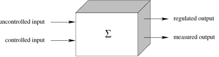
[image:25.612.113.475.484.578.2]

we indicate those variables which model the influence of the exterior world on the physical system and can be of different types - either controlled inputs or uncontrolled inputs (for instance, disturbances). By “outputs” we mean those variables with which the system acts on the exterior world. Sometimes the outputs are divided into two (not necessarily mutually disjoint) sets of variables. Those which are actually measured are calledmeasurements and those which must be controlled in order to meet specified requirements are called regulated (Figure 2.1). The vector spaces of the inputs and outputs

Figure 2.1: External Variables

signals U, Y are called input-space and output-space, respectively.

(26)

t and if c) the output value at time t is completely determined by the simultaneous input and state values. The vector space of all states of a system following the previous properties is denoted asX and is called state-space of the system.

A linear time invariant multivariable system, i.e., if {(x(t0), u(t)), t≥t0}

im-plies the outputy and {(Ta(x(t0)), Ta(u(t))), t≥t0}implies Ta(y₁) (whereTa

denotes the displacement operator that transfers bya− time units the state, the input and the output vectors to the right-hand side if the input and the output spaces are closed under these displacements) is represented in the time domain by the state variable model

S(A, B, C, D) :

˙

x(t) =Ax(t) +Bu(t), A∈_Rn×n_, _B _∈

Rn×k

y(t) = Cx+Du(t), C ∈_Rm×n_,_D_∈

Rm×k (2.1)

MatrixAis called theinternal dynamics matrix of the system and matricesB, C

are called input ( or actuator ) and output ( or sensor ) matrices respectively, with rankB = k, rankC = m and they express the so-called coupling of u, y. Furthermore, if matrixDis equal to the zero matrix, thenS(A, B, C, D) is called strictly proper.

Time-invariant systems are an equivalence class in the family of linear systems. In general, functions defined on a model which remain the same under certain types of transformations are called system invariants and are usually described by models with the simplest possible structure, i.e., the least number of param-eters, which are called canonical forms [Kar. 1]. Canonical forms, corresponding to representation transformations, provide a vehicle for model identification since they contain the minimal number of parameters within a given model structure to be defined. For control analysis and synthesis, aspects of the structure (as it is expressed by the system invariants) characterize the presence or absence of certain system properties; the type and values of invariants provide criteria for solvability of a number of control synthesis problems. In the area of control de-sign, the types and values of invariants frequently impose limitations in what it is possible to achieve. Although the link between system structure and achiev-able performance, under certain forms of compensation, is not explicitly known, system structure expresses in a way the potential of a system to provide certain solutions to posed control problems. More results with regard to canonical state space representation may be found in [Kar. 1], [Kar.& Vaf. 13].

On the other hand, the choice of a state for a system is not unique. However, there are some choices of state which are preferable to others; in particular, we look for vectorsx with the least dimension.

(27)

dimension of the smallest state vector, is called the McMillan degree of the system. Furthermore, systems which can be described with a finite number of variables are called finite-dimensional systems or infinite-dimensional otherwise.

In this thesis, we will deal with continuous-invariant time, finite-dimensional, linear systems of the form (4.19). For equivalent representations and for the parametrization problems that these systems appear in specific applications, one may refer to [Kar.& Vaf. 13], [Kar. & Mil. 12].

Remark 2.2.1. If s=d/dt denotes the derivative operator, then (4.19) may be expressed as

P(s)w₁(t) =w₂ (2.2)

where

P(s) :=

sIn−A −B

−C −D

, w₁(t) :=

x u

, w₂ :=

0

−y

The polynomial matrixP(s) is a special type of polynomial matrix, called system matrix pencil, [Kar.& Vaf. 13]. In general, matrix pencils appear as linear oper-ators of the type sF −G where s is an intermediate, frequently representing the Laplace transform variable and they are naturally associated with state-space type problems. They are used for state space calculations and geometric system theory and they provide a unifying framework for the study of the geometric properties of both proper (matrix D is constant) and singular systems (systems of infinite condition number), by reducing problems of singular system theory to equivalent problems of proper system theory, [Kar. 2], [Kal. 1], [Kar. 3]. Pencil matrices have been also used in the well-known Algebraic Eigenvalue Problem [Wilk. 1].

2.3 The Transfer Function Matrix

If one is not interested in the internal dynamics of a system, then the input-output system is basically just a map which associates with any input signal, the corresponding output signal. Specifically, ifx(t= 0) = 0 are the initial conditions for the states, the Laplace transform of system (4.19) implies,

S(A, B, C, D) :

sx(s) =Ax(s) +Bu(s)

y(s) =Cx(s) +Du(s) (2.3)

where by eliminating the states we obtain

y(s) = C(sIn−A)−1B+D

u(s) (2.4)

Definition 2.3.1. [Kai. 1] The m×k matrix

(28)

is called the transfer function or transfer matrix of the state space model (4.19) and describes how the system transforms an input est _{into the output} _G₍_s₎_est_.

Furthermore,G(s)is called proper ifG(∞)is a finite constant matrix and strictly proper if G(∞) = 0; if at least one entry of G(s) is infinity, then G(s) is called non proper.

The set of proper rational functions is denoted by _Rprf and for every G(s)∈

Rmprf×k[s] there always exists a state space model S(A, B, C, D) such that (2.5)

holds. Such state-space models are called realizations of G(s).

Definition 2.3.2. [Kai. 1] The realization with the least possible order is called minimal realization and this order is called the MacMillan degree of G(s).

Remark 2.3.1. For an non proper system, it can be shown, [Lew. 1], that it achieves a realization of the form Ex˙ = Ax +Bu, y = Cx, when E is not invertible.

It is easily shown that G(s) may take the form G(s) = N(s)D−1₍_s_{) which}

is called Polynomial Matrix Fractional Description. Moreover, if the degree of detD(s) is minimal amongst all other matrix fraction descriptions, then this description is called irreducible.

2.3.1 Stability, Controllability and Observability

From the definition of the transfer function and the results on zeros and poles, it is evident that the poles of G(s) must be contained among the eigenvalues of

A. In this section, we see that the poles ofG(s) are actually contained among the controllable andobservable eigenvalues of A, as only the controllable and observ-able part of the realization contributes to the transfer function. For this purpose, we briefly summarize at first the basic definitions and results, on controllability, stability and observability for a system S(A, B, C, D).

Definition 2.3.3. [Hin. & Pri. 1] Let a T- time domain dynamical system and

t0 ∈ T.

a) A state x_e is called equilibrium state (or equilibrium point) if

x(t) =x_e, ∀t∈ T

b) x_e is called asymptotically stable if

i) ∀ >0, ∃δ1 >0 : kx(t0)−xek< δ1 ⇒ kx(t)−xek< , ∀t ≥t0.

ii) ∃δ2 >0 : kx(t0)−xek< δ2 ⇒x(t)→xe, t→ ∞.

(29)

Theorem 2.3.1. [Hin. & Pri. 1] A dynamical system is Lyapunov - stable if and only if all eigenvalues of the matrix A of the respective autonomous system, have non positive real part and those whose real part is zero are simple structured. If all eigenvalues of A are negative then x_e is asymptotically stable.

Next, we recall the notion of controllability, i.e., whether and how we may choose the input so as to move the system fromx(0) = 0 to a desired target state

x(t1) =x1 at a given time t1.

Definition 2.3.4. [Kai. 1] Let the system S(A, B) : ˙x=Ax+Bu

i) S(A,B) is called controllable or (A, B)− controllable at a time t=t0 if

∀x₀, x₁ ∈_Rn_, _∃_u₍_t₎_|

[t0,t1], t1 ∈(t0,∞) : x(t0) =x0, x(t1) =x1

Otherwise, it is called uncontrollable.

ii) The eigenvalues λi, i= 1,2, ..., n of A for which

rank (λiIn−A, B) = n (2.6)

are called controllable eigenvalues (or modes) of the system.

iii) A system whose all uncontrollable eigenvalues are stable is called stabiliz-able.

For continuous time systems, the notion of controllability coincides with the notion ofreachability and the two terms are used equivalently. In case of discrete systems this is not possible, since matrix A may not be invertible.

Observability, on the other hand, is a measure for how well internal states of a system can be inferred by knowledge of its external outputs. The observability and controllability of a system aredual notions, i.e., controllability provides that an input is available that brings any initial state to any desired final state whereas observability provides that knowing an output trajectory provides enough infor-mation to predict the initial state of the system.

Definition 2.3.5. [Kai. 1] Let S(A, C) be the system (4.19) for D= 0.

i) S(A, C) is called observable or (A,C)- observable at [t0, tF] if for an input

u(t)and an outputy(t)we get a unique statex(t0) = x0. If one of the states

of x does not satisfy the previous rule, the system is called unobservable.

ii) The eigenvalues λi, i= 1,2, ..., n of A for which

rank

λiIn−A

C

=n (2.7)

(30)

iii) A system whose all unobservable eigenvalues are stable is called detectable.

Next we discuss the fundamental notions of poles and zeros of a system which are closely related to the notions described in this section.

2.3.2 Poles and Zeros

The poles and zeros of a system play an important role for its study; Poles could be described as the characteristic of the internal dynamical machinery of the system while zeros are the characteristic of the ways in which this dynamical machinery is coupled to the environment in which the system is embedded, and are associated with specific values of complex frequency at which transmission through the system is blocked. In picturesque terms, poles can be thought of as associated with system resonances coupled to input and output and zeros as as-sociated with anti-resonances at which propagation through the system is blocked.

Loosely speaking, multivariable poles and zeros are resonant and anti-resonant frequencies respectively, that is to say they are frequencies whose transmission explodes with time, or whose transmission is completely blocked. This, of course, is intuitively appealing since it forms a natural extension of the definitions given for the scalar case, where the poles and zeros of a scalar transfer function are defined as the values of the complex frequency s for which the transfer function gain becomes ∞, or 0 correspondingly. The inversion of roles of poles and zeros suggested by their classical complex analysis definition motivates the dynamic (in terms of trajectories) properties of zeros. The physical problem used to de-fine multivariable zeros is the “output zeroing” problem, which is the problem of defining appropriate non-zero input exponential signal vectors and initial condi-tions which result in identically zero output. Such a problem is the dual of the “zero input” problem defining poles, which is the problem of defining appropriate initial conditions, such that with zero input the output is a nonzero exponential vector signal. Those two physical problems emphasize the duality of the roles of poles and zeros.

Definition 2.3.6. [Kar. 4] Let the transfer functionG(s)ofS(A, B, C, D). Then,

i) s =s0 is a pole ofG(s), if the denominator of some entry of G(s) becomes

zero at s0.

ii) s = s1 is a zero of G(s) if G(s) drops rank at s = s1, or equivalently, if

there is a rational vector u(s) such that u(s1) is finite and nonzero and

lims→s1(G(s)u(s)) = 0.

Example 2.3.1. Let

G(s) =

1 _s₋1₂

0 1

(31)

It is clear that G(s) has a pole at s = 2, but it may not be immediately obvious that it also has a zero at s = 2. We observe that while s is approaching 2, the second column ofG(s) approaches alignment with the first column, so the rank of

G(s) approaches 1, i.e., there is a rank drop at s = 2. To confirm this, we may choose

u(s) =

−1

s−2

Then, u(2) is finite and nonzero and lims→2(G(s)u(s)) = 0.

Furthermore, the multiplicity associated with each pole and zero is not unique as in the single- variable case; each pole is associated with a set of multiplicities, e.g., if

G(s) = diag

s+ 2 (s+ 3)2,

s

(s+ 2)(s+ 3)

then we see that G(s) has poles at −3 of multiplicity 2 and 1 respectively. The concepts of pole, and zero have emerged as the key tools of the classical methods of Nyquist-Bode and root locus for the analysis and design of linear, single-input, single-output (SISO) feedback systems. The development of the state space S(A,B,C,D) description, transfer function G(s) description, and complex variable, (g(s), algebraic function) methods for linear multivariable systems has led to a variety of definitions for the zeros and poles in the multivariable case as Definition 2.3.6 and the emergence of many new properties. The variety and diversity in the definitions for the zeros and poles is largely due to the differences between alternative system representations the difference in approaches used, the objectives and types of problems they have to serve. A classic immediate method for the derivation of all poles and zeros without having to test any properties is via the Smith-MacMillan form [Kai. 1];

Theorem 2.3.2. (Smith-MacMillan) For any G(s)∈ _Rm×k _{there exist non}

sin-gular, square polynomial matrices P1, P2, det(Pi) = ci ∈ R\ {0}, i = 1,2 such

that

P1(s)G(s)P2(s) = diag

f1(s)

g1(s)

,f2(s) g2(s)

, ...,fr(s) gr(s)

, r= rank (G(s)) (2.8)

where fi, g(i), i = 1,2, ..., r are co-prime, monic polynomials such that fi+1 =

λifi, gi =κigi+1, i= 1,2, ..., r−1 for some λi, κi ∈R.

MatricesPi(s), i= 1,2 are calledunimodular and the roots of the numerator

polynomials fi(s) in (2.8) are the zeros whereas the roots of the gi(s) are the

poles of G(s).

(32)

for transfer function models the pole zero structure is introduced by the Smith-McMillan form. Such links reveal the poles as invariants of the alternative system representations under a variety of representation and feedback transformations. The strong invariance of zeros (large set of transformations) makes them critical structural characteristics, which strongly influence the potential of systems to achieve performance improvements under compensation.

From the Polynomial Matrix Fractional Description of G(s) we discussed in sec-tion 2.3, we may have:

G(s) = NR(s)D−R1(s) = DL(s)NL−1(s) (2.9)

where NR(s) ∈ Rm×k[s], DR(s) ∈ Rk×k[s] and NL(s) ∈ Rm×k[s], DL(s) ∈

Rm×m[s] are the so called Right Polynomial Matrix Fractional Description and

Left Polynomial Matrix Fractional Description of G(s) respectively when matri-cesDR, DL are invertible. This description of the transfer function gives another

alternative characterization of the poles and zeros of G(s); the poles ofG(s) are the roots of the polynomial det(DL(s)) = c(DR(s)), c ∈ R\ {0} and the zeros

are the roots of the product of the invariant polynomials ofNL(s) or NR(s).

Remark 2.3.2. The zeros ofG(s) are often called transmission zeros in order to distinguish them from another fundamental category of zeros, the invariant zeros, [MacFar. & Kar. 1], which are the zeros of the polynomial matrix

P(s) :=

sIn−A −B

C D(s)

(2.10)

where matrixP(s) is obtained by the necessary and sufficient condition

P(s)

x₀ v

= 0 (2.11)

which has to hold true in order an input of the form u(t) = vH(t)eat_{, a} _∈

C for

a system S(A, B, C, D(s)) to yield

u(t) =vH(t)eat, y(t)≡0, t >0 wherex₀ ∈_Rn _{is the initial state condition vector,} _v _∈

Rk andH(t)the Heaviside

unit-step function. A third group of zeros was introduced in [Ros. 1] which were named input-output decoupling zeros and they are obtained as the zeros of the invariant polynomial matrices

P1(s) := (sIn−A, B), P2(s) :=

sIn−A

C

(33)

respectively. The input-decoupling zeros correspond to the zeros of[DL(s), NL(s)]

and the output-decoupling zeros to the zeros of[DR(s), NR(s)]t for a left-right

co-prime MFD ofG(s)sinceNL(s), NR(s)have essential parts of Smith form defined

by the matrixdiag(f1(s), ..., fr(s))andDL(s), DR(s)have essential parts of Smith

form defined by diag(g1(s), ..., gr(s)), [Kar. 2] and for this reason they are also

called Smith-zeros. Both of them are associated with the situation where some free modal motion of the system state, of exponential type, is uncoupled from the system’s input or output. Note that pencils P1(s), P2(s) are the same matrices

which were used in (2.6) and (2.7) to test the controllability and the observability of a system, respectively. The sum of the transmission zeros and decoupling zeros is called system zeros of (2.10).

Finally, we have the following result that connects the notions of controllabil-ity and observabilcontrollabil-ity of the previous section with the poles and zeros.

Theorem 2.3.3. [Kar. 4] The following hold true:

i) If a system is controllable and observable, then the sets of invariant zeros and transmission zeros are the same.

ii) Every uncontrollable eigenvalue is a system zero.

iii) Every unobservable eigenvalue is a system zero.

iv) The spectrum σ{A−BD−1_C_} _{is precisely equal to the set of the systems}

transmission zeros.

v) The poles of the transfer function G(s) are precisely equal - in location and multiplicity - to the controllable and observable eigenvalues of A and the multiplicity indices associated with a pole of G(s) are precisely the sizes of the Jordan blocks associated with the corresponding eigenvalue of A.

Every square system (same number of input and outputs) has zeros (finite and/or infinite); however, non-square systems generally do not have zeros and this is an important difference with the poles that exist independent from input, output dimensionalities. Although non-square systems generically have no zeros, they have “almost zeros”; this extended notion expresses “almost pole-zero can-celations” and it is shown in [Kar. 4] that in a number of cases behaves like the exact notion.

(34)

2.4 Composite Systems and Feedback

On the general state-space description (4.19), a number of transformations may be applied, which are of the representation type (different coordinate sys-tems) and expressed by coordinate transformations, and of the feedback com-pensation type; the latter is made up from state, output feedback and output injection. These transformations are denoted below, [Kar.& Vaf. 13]:

(i) R :k×k input coordinate transformation, detR 6= 0.

(ii) T :m×m output coordinate transformation, detT 6= 0.

(iii) Q, Q−1 :n×n pair of state coordinate transformations, detQ6= 0. (iv) T :m×k constant output feedback matrix.

(v) L:n×k state feedback matrix.

(vi) T :n×n output injection matrix.

The above set of transformations (R, T, Q−1_{, L, K}_{) when applied on the original}

system S(A, B, C, D) described by the matrix P(s) in (2.10), i.e.,

P(s) =

sIn−A −B

C D

then a new system S0(A0, B0, C0, D0) is produced, described by

P0(s) :=

Q−1 _K

0 T

sIn−A −B

C D

Q 0

L R

(2.13)

As shown in [Kar.& Vaf. 13],P(s), P0(s) are related by a certain form of equiv-alence, which is defined on matrix pencils. Such transformations are referred to as the full set of state-space transformation, or as the Kronecker set of transfor-mations. In [Kar.& Vaf. 13] there are various representations the Kronecker set of transformations, such as the so-calledS(A) description where the transforma-tions on the T(s) pencils are similar, i.e., T0(s) = Q−1₍_sI

n −A)Q. Before we

end this section, we briefly present the feedback compensation on composite sys-tems, in order to generalize some of the results presented in the previous sections.

(35)

output space Yi, i ∈ N := {1,2, ..., n}, n ∈ N, the direct sum is the system

(A, B, C, D) with state space X, input space U and output spaceY given by

X =

n

Y

i=1

Xi, U = n

Y

i=1

Ui, Y = n

Y

i=1

Yi (2.14)

and

A=

n

M

i=1

Ai, B = n

M

i=1

Bi, C = n

M

i=1

Ci, D = n

M

i=1

Di (2.15)

Hence, the direct sum is just a collection of uncoupled systems. This is not the case if the subsystems Σi are interconnected within the composite system or if the

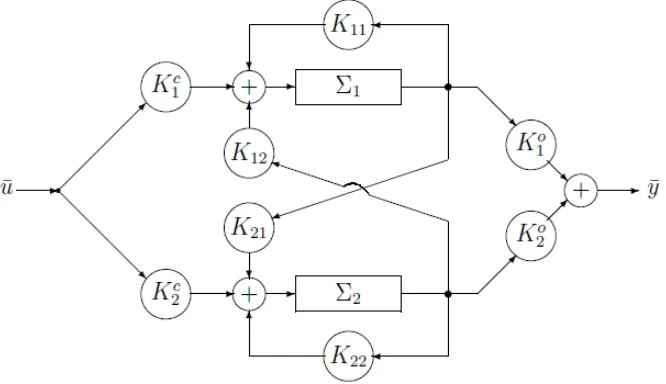
original system is interconnected with itself (feedback). In this section we examine the second case for two subsystems, the original system (plant) and the system of the controller as in the following figure. The input, state and output spaces of the composite system are denoted by U, X, Y and by K = (Kij)i,j∈N, K

c i :

U → Ui, Kio :Yi → Y we denote the so called matrix of interconnections of the

[image:35.612.128.461.374.566.2]

subsystems and the input and output coupling matrices respectively.

Figure 2.2: General composite system of two subsystems

If we connect the output of Σ1 to the input of Σ2 and the output of Σ2 to the

input of Σ1, then the above configuration 2.2 is calledDynamic Output Feedback.

Thus, by settingui ≡ui ∈ U, yi ≡y_i ∈ Y and u∈ U, the couplings u2 =y1 and

u1 =y2+ulead to the feedback equations

u1 =C2x2+D2(C1x1+D1u1) +u, u2 =C1x1+D1(C2x2+D2u2+u) (2.16)

These equations can be solved foru₁andu₂ if and only if the matricesIU1−D2D1,

(36)

condition for the feedback configuration and if it is satisfied, the feedback system is said to bewell defined. It has input space U =U1, output spaceY =Y1, state

space X =X1× X2 and its system equations are given by the data

A=

A1+B1(In−D2D1)−1D2C1 B1(In−D2D1)−1C2

B2(In−D1D2)−1C1 A2 +B2(In−D1D2)−1D1C2

,

B =

B1(In−D2D1)−1

B2(In−D1D2)−1D1

,

C = C1+D1(In−D2D1)−1−D2C1 D1(In−D2D1)−1C2

D=D1(In−D2D1)−1

Next theorem provides a necessary and sufficient for a composite system to be proper.

Theorem 2.4.1. [Vid. 1] Let G1(s), G2(s) be the transfer matrices of a plant

and its controller.

i) The transfer function matrix of the composite system is

G(s) := G1(s)(In−G2(s)G1(s))−1 (2.17)

ii) G is proper if and only if

t(∞)∈_R (2.18)

where t(s) = det(In−G1(s)G2(s)).

The next two results [Chen. 1] now generalize the notions of stability, con-trollability and observability for the general feedback configuration.

Definition 2.4.1. A composite well-posed system is called internally stable if its respective autonomous system x˙ =Ax is asymptotically stable.

Proposition 2.4.1. Let a composite well-posed system Σ.

i) Σ is controllable, if and only if {Σ1, Σ2} are both controllable.

ii) Σ is observable, if and only if {Σ1, Σ2} are both observable.

iii) Σ is stabilizable, detectable if and only if both {Σ1, Σ2} are stabilizable,

detectable.

(37)

2.5 Frequency Assignment Problems

The problem of pole placement for systems of the form (4.19) in order to obtain the required stability and other properties, is a core problem in Systems Theory. In this section, we see that these two problems along with other frequency assignment problems such as the design of an asymptotic observer and the prob-lem of zero assignment by squaring down, lie in a wider category of probprob-lems, the so called Determinantal Assignment Problem [Kar. & Gia. 5], [Kar. & Gia. 6].

Definition 2.5.1. (Pole Assignment by state feedback) [Won. 1]. Let a state space model of the form (4.19). The Pole Assignment by state feedback problem is defined as the derivation of a matrix K ∈ _Rk×n_, _rank_K ₌ _k_{, such that the}

equation:

˙

x= (A−BK)x+Bu, A ∈_Rn×n_{, B} _∈

Rn×k (2.19)

has the following characteristic polynomial:

det(sIn−A+BK) = det(M(s) ˜K) = a(s) (2.20)

wherea(s)is an arbitrary polynomial ofn degree and M(s) = (sIn−A, B), K˜t =

(It n, Kt).

This problem has been completely solved in [Won. 1], where the following theorem was proved.

Theorem 2.5.1. A system is (completely) pole assignable by state feedback, if and only if the system is controllable.

In [Kai. 1] the problem of the asymptotic observer has been established as the dual problem of the state feedback problem:

Definition 2.5.2. (Design of an asymptotic observer) [Kai. 1]. The problem of the asymptotic observer design is defined as the derivation of a matrixT ∈_Rn×m_,

such that

det (sI −A+T C) = det

˜

T C(s)

a(s) (2.21)

wherea(s)is an arbitrary polynomial ofndegree andCt(s) = ((sIn−A)t, Ct), T˜=

(In, T).

Due to the duality of the state feedback problem and the asymptotic ob-server’s design, the latter is solvable if and only if the system is observable.

(38)

Definition 2.5.3. (Pole Assignment by constant output Feedback) [Kim. 1]. The problem of pole assignment by constant output feedback is the derivation of a matrix F ∈_Rk×m _{such that}

det(sIn−A−BF C) = det(sIn−A) det(In−(sIn−A)−1BF C) =

= det(sIn−A) det(In−G(s)F) = det (FRTR(s)) =

=a(s) (2.22)

where a(s) is an arbitrary polynomial of n degree and

FR= (Ik, F)∈Rk×(m+k), TR(s) =

DR(s)

NR(s)

are obtained by the Right Polynomial Matrix Fractional Description of the respec-tive transfer function.

The problem has been mostly examined generically, i.e., for almost all polyno-mials a(s), [Wil. & Hes. 1]. Note that if there exist real matrices F that satisfy the above form (2.22) of the closed-loop characteristic polynomial we refer to the problem as completely pole assignable by static output feedback, whereas if there exist open dense sets of real coefficients (a1, ..., an) defined by the polynomial

a(s) for all matrices F that satisfy (2.22), then we refer to the generically pole-assignable by static output feedback problem.

Most authors have examined the problem in terms of solvability and

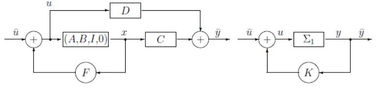
assignabil-Figure 2.3: Static state and output feedback

ity conditions; From [Dav. & Wan. 1], [Kim. 1] and [Ser. 1] where the sufficient condition m+k ≥ n+ 1 for a generic pole assignment system with m outputs,

[image:38.612.99.484.461.552.2]

The approximate determinantal assignment problem

City, University of London Institutional Repository

Citation:

This is the accepted version of the paper.

This version of the publication may differ from the final published

version.

Permanent repository link:

Link to published version:

Copyright and reuse: City Research Online aims to make research

outputs of City, University of London available to a wider audience.

Copyright and Moral Rights remain with the author(s) and/or copyright

holders. URLs from City Research Online may be freely distributed and

linked to.

THE APPROXIMATE

DETERMINANTAL ASSIGNMENT

PROBLEM

George Petroulakis

A thesis submitted for the degree of Doctor

of Philosophy

City University London, School of

Mathematics, Computer Science and

Engineering, EC1V OHB, London, United

Kingdom

Contents

Acknowledgements

Nonemclature

Chapter 1

Introduction

Chapter 2

Preliminary Results from

Systems Control Theory

2.1

Introduction

2.2

State Space Models

2.3

The Transfer Function Matrix

2.3.1

Stability, Controllability and Observability

2.3.2

Poles and Zeros

2.4

Composite Systems and Feedback

2.5

Frequency Assignment Problems