Evolution in a Changing Environment

City, University of London Institutional Repository

Citation

:

Baronchelli, A., Chater, N., Christiansen, M. H. and Pastor-Satorras, R. (2013). Evolution in a Changing Environment. PLoS ONE, 8(1), doi: 10.1371/journal.pone.0052742

This is the unspecified version of the paper.

This version of the publication may differ from the final published

version.

Permanent repository link:

http://openaccess.city.ac.uk/2654/

Link to published version

:

http://dx.doi.org/10.1371/journal.pone.0052742

Copyright and reuse:

City Research Online aims to make research

outputs of City, University of London available to a wider audience.

Copyright and Moral Rights remain with the author(s) and/or copyright

holders. URLs from City Research Online may be freely distributed and

linked to.

City Research Online: http://openaccess.city.ac.uk/ [email protected]

arXiv:1304.6375v1 [q-bio.PE] 23 Apr 2013

Evolution in a changing environment

Andrea Baronchelli1, Nick Chater2, Morten H. Christiansen3, Romualdo Pastor-Satorras4,∗

1 Laboratory for the Modeling of Biological and Socio-technical Systems, Northeastern University, Boston MA 02115, USA

2 Behavioural Science Group, Warwick Business School, University of Warwick, U.K.

3 Department of Psychology, Cornell University, USA, and Santa Fe Institute, USA

4 Departament de Fisica i Enginyeria Nuclear, Universitat Politecnica de Catalunya, Campus Nord B4, 08034 Barcelona, Spain

∗ E-mail: [email protected]

Abstract

We propose a simple model for genetic adaptation to a changing environment, describing a fitness landscape characterized by two maxima. One is associated with “specialist” individuals that are adapted to the environment; this maximum moves over time as the environment changes. The other maximum is static, and represents “generalist” individuals not affected by environmental changes. The rest of the landscape is occupied by “maladapted” individuals. Our analysis considers the evolution of these three subpopulations. Our main result is that, in presence of a sufficiently stable environmental feature, as in the case of an unchanging aspect of a physical habitat, specialists can dominate the population. By contrast, rapidly changing environmental features, such as language or cultural habits, are a moving target for the genes; here, generalists dominate, because the best evolutionary strategy is to adopt neutral alleles not specialized for any specific environment. The model we propose is based on simple assumptions about evolutionary dynamics and describes all possible scenarios in a non-trivial phase diagram. The approach provides a general framework to address such fundamental issues as the Baldwin effect, the biological basis for language, or the ecological consequences of a rapid climate change.

Introduction

rapidly for genes to follow [8]. This paper provides an analytical framework for addressing these issues.

The study of evolution and adaptation in a fluctuating environment from the perspective of population genetics has been hampered by the mathematical difficulty of the problem [9]. Various modeling attempts have focused on the conditions leading to adaptation, or lack thereof, from the perspective of the Baldwin effect (e.g. [10, 11]), or on species distributions in the presence of environmental stresses (e.g. [12–14]), but a general picture is still lacking. These models, in fact, while useful and interesting, are usually defined in terms of a large number of parameters, which compromise the possibility of studying them thoroughly from an analytical point of view, or of achieving fundamental insights into the problem at hand. Other work has instead followed the quasi-species approach [15–18], but also these models are in general characterized by considerable mathematical complexity.

Here we propose a stochastic interacting particle model that captures the most basic fea-tures characterizing evolution in a dynamic environment. The model is simple and analytically tractable at a mean-field level, and provides a general view of the gene-environment dynam-ics. Our work follows the statistical physics approach to evolutionary dynamics, which has become increasingly influential [19–22], clarifying, for example, crucial issues such as the role of the topology defining the interaction patterns in an evolving population [23] or system-size effects [24].

The model describes a large population of n individuals and an external, environmental feature. Individuals are divided in three general types: “specialists” who are adapted to the environment, “generalists” whose fitness is independent of the environment, and “maladapted.” We assume that a complex network of genes codes for the ability to adapt to a specific feature of the environment. For example, we might focus on the linguistic environment, which has many specific forms corresponding to particular languages, such as English. A perfect tuning of this network would allow a “specialist” individual to learn very rapidly the specific language for which it is optimized, thus increasing her fitness (ability to survive and reproduce). Here we can say that the genes are aligned with a specific feature of the environment [11]. However, specialization comes with a cost, reducing the flexibility of the specialized genome [25]. Even a slight environmental change might cause problems to the offspring inheriting a genetic machinery evolved for the original, but now different, environment. The new individual would in fact be

misaligned (maladapted) and her fitness would be lowered. For this reason we include in the model also a third kind of genomes, namely the neutrals (or “generalists” [26]), for which the fitness of an individual is independent of the specific environment. Note that working with just one environmental feature corresponds to the assumption, standard when modeling complex biological phenomena [27], that different features of the environment have roughly independent impacts on fitness.

The dynamics of the model is defined in terms of evolutionary rules that depend on three basic parameters: The genetic mutation rate m, the rate of environmental change ℓ, and a parameter

p, indicating the probability that an environmental change could lead to conditions favorable for previously maladapted individuals. As we will see, the probabilitypturns out to induce only small corrections in the biological limit p → 0. In terms of the remaining parameters m and

of the rate of environmental change. This phase diagram describes the general conditions for microevolutionary adaptation in the presence of environmental stresses, and explains different empirical observations of adaptation in changing environments in a single framework.

Results

Model definition

The model is defined in terms of three different types, namelyS,N, andM, that represent Spe-cialized, generalist/Neutral, and Maladapted individuals, respectively. Our aim is to describe a population in which the environment changes. Thus, thinking in terms of a theoretical fitness landscape [29], we assume that it exhibits a maximum whose position changes whenever there is an environmental variation, i.e., the maximum represents a moving target. The main simpli-fication of our model, as opposed to standard quasi-species approximations [15, 18], consists in considering the class of specialists S not as a fixed genome, but as the set of those genomes which are closer to the maximum of the fitness landscape, whatever the position of this maxi-mum might be. In this theoretical fitness landscape we assume also the presence of a secondary, local, maximum, of lower height, representing the neutral genomes which are not affected by environmental changes. The position of this secondary maximum is considered static, since neutrals do not react to changes in the environment. From this perspective, our model borrows from quasi-species models in multiple-peaked landscapes [30], with the proviso that the absolute maximum moves in time, and we do not focus on fixed genomes, but on the set of those close to the maxima.

In mathematical terms, the class S can thus be described as the set of genomes that are close to the principal maximum, by a distance ǫS. Analogously, species N represents the set of

genomes close to the perfectly neutral genome (the secondary fixed maximum), by a distance

ǫN. Finally, the set M is composed of the remaining possible genomes. We assume a haploid

reproduction system, with a fitness for each class fα, satisfying the restriction fM < fN < fS.

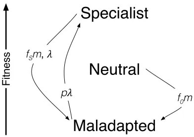
We consider these fitnesses as constant, independent of the environmental changes. At a mean-field level, assuming homogeneous mixing, the dynamics of the model is defined as follows (see Fig. 1): Reproduction is performed by selecting an individual with probability proportional to its fitness, as in standard haploid models (i.e., the Moran process [31]). The individual then produces an offspring which is equal to itself with probability 1−m, and that mutates to a different type with probability m. Conservation of individuals is achieved in reproduction by eliminating a randomly chosen individual. Crucially, all genetic mutations are assumed to be harmful, because the probability that they will lead to an increase of fitness is negligible [32]. Therefore, a genome of type S or N, when mutating, reproduces into a type M, while M

the shift could have a beneficial effect on other previously maladapted individuals, who were, in genomic space, far from the previous position of the principal maximum but are now close to its present one. This effect, which we assume to be rarer, is implemented by choosing with a small probability p a maladapted individual (with probability ρM), which will become specialized.

Note that we neglect backward genetic mutations from M genomes to either S or N species. Thus, we are considering the most common scenarios in which beneficial mutations are much less frequent than harmful ones (see for example [33,34]). Moreover, from the rules of the model, the population sizenis constant. This restriction is not problematic for our purposes, since we are interested only in the ratios between the population densities of the different species. In what follows, however, we will consider the limit of an infinite population, n→ ∞, so that the presence of S and M individuals can be assumed to be non-zero at the outset due to generic variability in the population, even thought they may be few in number. As we will see, the solution to our equations does not depend on the initial fractions of the different genomes.

Mean-field rate equations

Let us defineραas the density of individuals in state α∈[S, N, M], satisfying the normalization

condition P

αρα = 1. At the mean-field level, disregarding spatial fluctuations and stochastic

fluctuations, and in the limit ofn→ ∞, a mathematical description of our model can be readily obtained in terms of rate equations for the variation of the densitiesρα. To construct those, we

consider that a genomeαincreases its number (i) when an individualαis chosen for reproduction and her offspring replaces an individual belonging to a genome β 6=α, without any mutation, i.e., with probability (1−m), or (ii) when a mutation event leads an individual with genome

β 6= α to reproduce into α. Conversely, a genome α decreases when one individual belonging to it is randomly selected for replacement. Additionally,S genomes may decrease their number due to a damaging change of the environment, while they can increase their number through a (rarer) beneficial environmental change. The corresponding rate equations take thus the form, writing explicitly all contributions to the change to each ρα,

˙

ρS =

fSρS

φ (1−ρS)(1−m)− fSρS

φ ρSm− fNρN

φ ρS(1−m)− fNρN

φ ρSm

− fMρM

φ ρS−ℓρS+ℓpρM,

˙

ρM = −

fSρS

φ ρM(1−m) + fSρS

φ (1−ρM)m− fNρN

φ ρM(1−m) + fNρN

φ (1−ρM)m

+ fMρM

φ (1−ρM) +ℓρS−ℓpρM,

˙

ρN = −

fSρS

φ ρN(1−m)− fSρS

φ ρNm+ fNρN

φ (1−ρN)(1−m)− fNρN

φ ρNm− fMρM

φ ρN,

where we have defined rate of environmental change ℓ= λ/(1−λ), the average fitness of the populationφ=P

some algebraic manipulations, the previous equations can be simplified to the form:

˙

ρS = ρS

h

−1 + (1−m) ˆfS−ℓ

i

+pℓρM, (1a)

˙

ρN = ρN

h

−1 + (1−m) ˆfN

i

, (1b)

˙

ρM = ρM

h

−1 + (1−m) ˆfM−pℓ

i

+m+ℓρS, (1c)

where we have defined ˆfα =fα/φ.

Equations (1) completely define the dynamics of the model at the mean field level. In the following we will analyze their solution in different limits.

Analytical solution

In the long term steady state, the solutions of this dynamical system are obtained by imposing the conditions ˙ρS = ˙ρN = ˙ρM = 0 on Eqs. (1), solving the ensuing algebraic equations, and checking

for the stability of the solutions, by looking at the eigenvalues of the Jacobian matrix, evaluated at the respective solution. The solutions obtained this way in the general case p >0 turn out to be quite complex, so in order to simplify the resulting expressions, we choose particular values of the fitnesses, namely fS= 2, fN = 1 andfM = 0.5, respecting their natural ordering. Solutions

for other values can be obtained using the same steps.

Case p6= 0

The algebraic equations ruling the steady state, obtained from Eqs. (1) by setting to zero the time derivatives, can be solved using a standard computational software package. This results in three sets of solutions, taking the form

S1             

ρN = 0

ρS =−

p

2ℓ(m(4−8p) + 12p−3) + (3−4m)2_{+ (4pℓ+ℓ)}2_{+ 4m−2pℓ+ℓ−3}

6(pℓ+ℓ+ 1)

ρM =

p

2ℓ(m(4−8p) + 12p−3) + (3−4m)2_{+ (4pℓ+ℓ)}2_{+ 4m+ 4pℓ+ 7ℓ+ 3}

6(pℓ+ℓ+ 1)

, S2             

ρN = 0

ρS =

p

2ℓ(m(4−8p) + 12p−3) + (3−4m)2_{+ (4pℓ+ℓ)}2_{−4m+ 2pℓ−ℓ+ 3}

6(pℓ+ℓ+ 1)

ρM =

−p2ℓ(m(4−8p) + 12p−3) + (3−4m)2_{+ (4pℓ+ℓ)}2_{+ 4m+ 4pℓ+ 7ℓ+ 3}

6(pℓ+ℓ+ 1)

, S3             

ρN =

2ℓ(mp+m+p)−2m−ℓ+ 1 (2p−1)ℓ+ 1

ρS =−

2mpℓ

2pℓ−ℓ+ 1

ρM =−

2m(ℓ−1) (2p−1)ℓ+ 1

Solution S1 describes a ρS density that is negative in the parameter region p >0, i.e., it is

an “unphysical” solution that does not describe any realistic scenario. Solution S₂ has nonzero densities in the whole parameter space, while solution S3 is physical only in the region

R=

0< m < 1

2 ∧0< p <

1−2m

2m+ 2∧ℓ≥

2m−1 2(mp+m+p)−1

. (2)

In order to find the relative stability of the physical solutionsS2andS3, we consider the Jacobian

matrix of the equation system Eqs. (1), taking the form

J =

   

−4(m−1)(ρM+2ρN)

(ρM+2ρN+4ρS)2 −ℓ−1

8(m−1)ρS

(ρM+2ρN+4ρS)2

4(m−1)ρS

(ρM+2ρN+4ρS)2 +pℓ

8(m−1)ρN

(ρM+2ρN+4ρS)2 −

2(m−1)(ρM+4ρS)

(ρM+2ρN+4ρS)2 −1

2(m−1)ρN

(ρM+2ρN+4ρS)2

4(m−1)ρM

(ρM+2ρN+4ρS)2 +ℓ

2(m−1)ρM

(ρM+2ρN+4ρS)2 −

2(m−1)(ρN+2ρS)

(ρM+2ρN+4ρS)2 −pℓ−1

   

.

We then compute the eigenvalues of matrix J, evaluated for the different solutions S2 and S3.

In any given region of parameter space, the stable solution (in the stationary limit) is the one possessing a negative largest eigenvalue. Examination of these eigenvalues, operation performed again with the help of standard computational software packages, leads to the solution:

•If (m, p, ℓ)∈ R:

            

ρN =

2ℓ(mp+m+p)−2m−ℓ+ 1 (2p−1)ℓ+ 1

ρS=

2mpℓ ℓ−2pℓ−1

ρM =

2m(ℓ−1) (1−2p)ℓ+ 1

. (3) •Otherwise:             

ρN = 0

ρS=

p

2ℓ(m(4−8p) + 12p−3) + (3−4m)2_{+ (4pℓ+ℓ)}2_{−4m+ 2pℓ−ℓ+ 3}

6(pℓ+ℓ+ 1)

ρM =

−p2ℓ(m(4−8p) + 12p−3) + (3−4m)2_{+ (4pℓ+ℓ)}2_{+ 4m+ 4pℓ+ 7ℓ+ 3}

6(pℓ+ℓ+ 1)

(4)

where Ris the domain in the parameter space defined in Eq. (2).

The analytical solutions given by Eqs. (3) and (4) are quite complex, and it is difficult to extract direct interpretations from them. However, the behavior of the solutions can be understood in the biologically relevant region of small p. Fig. 2 shows the densities ρα as a

function ofmor ℓ, at fixedℓandm respectively, for two values ofp, along with the value of the total fitnessφ=P

αραfα. In the upper left corner plot for each value ofp, we consider the case

m= 0.05, representative of the biologically relevant scenario of small mutation rate. Whenℓ is very small, most of the population stays aligned with the environmental feature andρS ∼1. As

ℓand smallm, trying to catch up with the rapidly evolving environmental feature is not a viable strategy, since the risk of producing a maladapted offspring becomes destructive. Interestingly the strategy adopted by the majority of the individuals guarantees the maximum average fitness in any given region of the (ℓ, m) plane, for every value of p. For large values of m (lower left plots), the situation is qualitatively different. For small ℓ, maladapted and neutral individuals are almost equally numerous. When ℓ increases beyond a threshold, neutral individuals again appear suddenly, but they are unable to overcome maladapted genomes. Only for large values of

pare neutrals capable to prevail over the specialists. The right plots for each value ofpin Fig. 2 show the evolution of the species’ densities as a function of mfor fixedℓ. In this case, for small

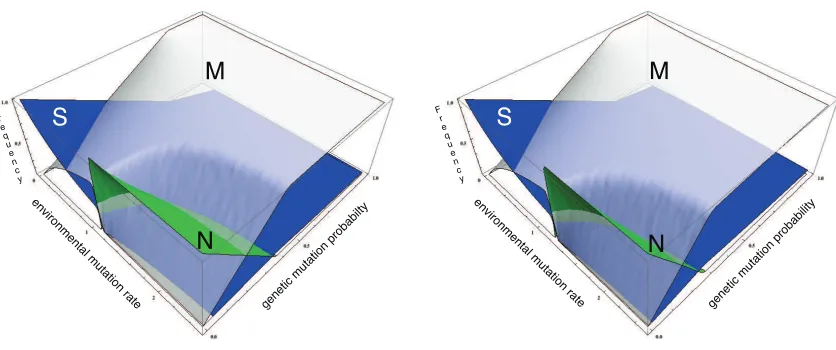
ℓneutrals are absent from the system, and there is a simple competition between specialists and maladapted, the former being predominant for small genetic mutation rates, but going extinct for large m. On the other hand, when the rate of environmental change is sufficiently large, we enter a new scenario in which neutrals are predominant for small m. Beyond a mutation rate threshold, however, neutrals suddenly become extinct, and their population is replaced by maladapted genomes, while specialists decrease their density for large m. Interestingly, in this region of largeℓ, specialists can survive even for very large mutation rates, close to 1, due to the effect of a nonzeropthat prevents their complete elimination. Fig. 3 shows the complete picture of the relative species’ abundances as as a function of m and ℓ for the previously considered values of p.

Case p= 0

A more precise mathematical characterization of the phenomenology discussed above, and in particular of position of the transitions taking place for different values of m and ℓ, can be obtained in the particular case p= 0. Here, qualitative arguments allow us to solve the model in a much simpler way, for general values of fS, fN and fM. This analysis, moreover, reveals

the role of p in the dynamics of our model. The relevant equations in thep= 0 case read

˙

ρS = ρS

h

−1 + (1−m) ˆfS−ℓ

i

, (5a)

˙

ρN = ρN

h

−1 + (1−m) ˆfN

i

, (5b)

˙

ρM = ρM

h

−1 + (1−m) ˆfM

i

+m+ℓρS. (5c)

To find their solution, we argue as follows: If m is very close to 1, all terms in square brakets in Eqs. (5) will be negative. Therefore, the only stable solution will be ρS =ρN = 0, ρM = 1,

for any value ofℓ. Under this conditions, the quantities within square brackets in Eqs. (5a) and (5b) take the form−1−ℓ+ (1−m)fS/fM and−1 + (1−m)fN/fM, respectively. Decreasing the

value ofm, the first solution withρM <1 will take place for the first of these values that become

zero. This occurs whenmis smaller than eithermc,1(ℓ) = 1−(ℓ+1)fM/fS ormc,2 = 1−fM/fN,

respectively. SincefM < fN, we have 0< mc,2 <1, and this transition will always be physical.

However, for ℓ > ℓc,1 = (fS−fM)/fM, we have mc,1(ℓ)<0 and it is not physical. In this case,

when ℓ > ℓc,1, if m < mc,2, ρS decays exponentially, and in the long time limit ρS = 0; the

the restricted normalization condition ρN +ρM = 1 leads to the solution ρN = 1−m/mc,2 ρM =m/mc,2, and ρS = 0. In the case ℓ < ℓc,1, which density ρS or ρN becomes first non-zero

depends on which threshold, mc,1(ℓ) or mc,2 is larger. Thus, if ℓ > ℓc,2 = (fS−fN)/fN, then

mc,2 > mc,1(ℓ). Therefore, when decreasing m, the first density to take a non-zero value isρN.

ρS decays again exponentially, so the solution is the same as in the case ℓ ≥ ℓc,1. Finally, for ℓ < ℓc,2,ρS is the first density to become non-zero when m < mc,1. The steady state solution

comes from imposing−1−ℓ+ (1−m) ˆfS = 0, leading toφ=fS(1−m)/(ℓ+ 1). In this region,

the factor in square brackets in Eq. (5b) becomes negative, indicating an exponential decay and a corresponding steady state value ρN = 0. We are therefore led to the solution, using the

normalization condition, ρS= (mc,1(ℓ)−m)/[ℓc,1(1−mc,1(ℓ))],ρM = 1−ρS.

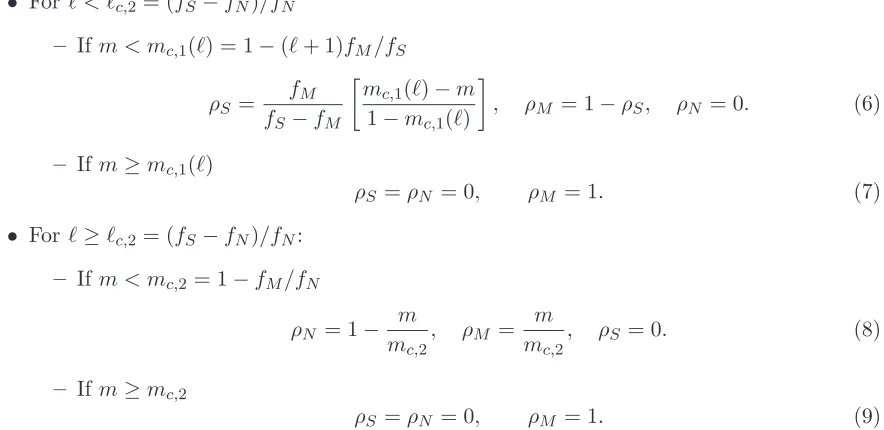
The final solution in this case can thus be summarized as follows:

• For ℓ < ℓc,2 = (fS−fN)/fN

– Ifm < mc,1(ℓ) = 1−(ℓ+ 1)fM/fS

ρS =

fM

fS−fM

mc,1(ℓ)−m

1−mc,1(ℓ)

, ρM = 1−ρS, ρN = 0. (6)

– Ifm≥mc,1(ℓ)

ρS=ρN = 0, ρM = 1. (7)

• For ℓ≥ℓc,2 = (fS−fN)/fN:

– Ifm < mc,2 = 1−fM/fN

ρN = 1−

m mc,2

, ρM =

m mc,2

, ρS= 0. (8)

– Ifm≥mc,2

[image:9.612.99.541.273.488.2]

ρS=ρN = 0, ρM = 1. (9)

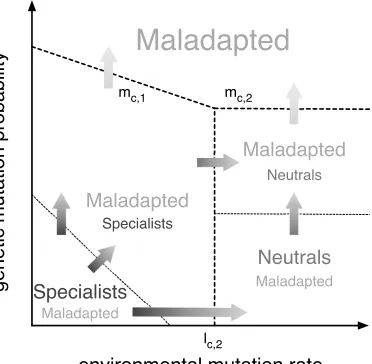
Fig. 4 sketches the phase diagram, as a function of m and ℓ, resulting from the previous equations. The different scenarios for small and large values of ℓ are now explicit. For small

ℓ < ℓc,2, specialist individuals (in the N class) are able to survive, and even dominate the

population, as long as the mutation rate is small. In fact, for m < mc,3(ℓ) =mc,1(ℓ)−ℓc,1[1− mc,1(ℓ)]/2, the density of specialists is larger than the density of maladapted individuals. For

largerm, the density of specialized genomes decreases, until it reaches theℓ-dependent threshold

mc,1(ℓ), leading to a continuous, second order, phase transition (akin to the error catastrophe

in quasispecies models [28]) beyond which the whole population becomes maladapted and thus prone to eventual extinction. In all of this region of small ℓ, neutral individuals are irrelevant. For small m, specialists perform much better, while for large m only maladapted individuals survive.

When ℓ increases, a different picture emerges. For fixed, small m < mc,2, the explicit

behavior of ρS as a function ofℓ, reads we can obtain from Eq. (6)

ρS =

fM

(ℓ+ 1)(fS−fN)

fS

fM

(1−m)−1−ℓ

forℓ < ℓc,2, and zero otherwise. Thus, when crossing ℓc,2, the density of specialized individuals

experiences a first order transition to extinction, with a jump of magnitude

∆ρS =

fN(1−m)−fM

fS−fM

. (11)

The sudden extinction of specialized individuals coincides with the abrupt emergence of neutrals, in a related first order transition for ρN with an associated jump

∆ρN =

fN(1−m)−fM

fN −fM

. (12)

In this large ℓregion, neutrals are able to cope with environmental change if the mutation rate is sufficiently small, again up to a maximum mutation rate mc,1, after which ρN continuously

becomes zero and only maladapted individuals can survive. These discontinuous transitions as a function ofℓat fixedmare reminiscent of the phenomenology observed in quasispecies models with higher order replication mechanisms [35]. We note, however, that transition as a function of m at fixedℓ are all continuous.

Fig. 5 shows the proportions of the three genomes along with the average fitness as function of m for fixed ℓ, and as a function of ℓ at fixed m (left panel), and the general scenario as a function of both m and ℓ (right panel). As it is clear, while an abrupt transition occurs at the level of the genome frequencies at ℓc,2 (ℓc,2 = 1 in Fig. 5), the average fitnessφ exhibits a

continuous behavior, decreasing monotonously from the maximum φ = fS for m = ℓ = 0 to

φ=fM for large values of m (when all the other genomes simply mutate intoM). Whenm is

fixed (left column, left panel), increasingℓcauses an increase ofM genomes and a simultaneous decrease inρS andφ. Asℓ=ℓc,2, howeverSgenomes disappear as the neutral genomes abruptly

appear. The latter guarantees a constant value of φ. M genomes are constantly created due to the genetic mutation rate, but their fitness is lower so they do not reproduce frequently. This scenario is stable, and any further increase in l does not produce any effect. The role of m is better understood at fixed values of ℓ. When ℓ < ℓc,2 (top panel) increasing mdeteriorates the

fitness of the population since S genomes are substituted by M ones, which eventually become fixed (ρM = 1 asm=mc,1 = 0.725 in figure). A similar behavior is observed forℓ > ℓc,2(bottom

panel), but here the M genomes take the place of the N genomes, till the latter disappear at

mc,2= 0.5 for the values of the simulations.

The crucial difference between the cases p 6= 0 and p = 0, as can be observed from the comparison of Figs. 2 and 5 is the effect of a positive density of specialists for largem andℓ. In the case p = 0, the density ρS goes to zero after the corresponding transition, specialist being

Discussion

The model presented in this paper shows that a genetic adaptation to a specific form of an environmental feature is profitable only as long as the rate of change in the environment is not too fast. Indeed, a phase transition determines the onset of a different regime in which a neutral strategy is advantageous. The critical value of the environmental rate separating the two phases is proportional to the difference between the fitness of the neutral and specialist individuals. This analysis is the consequence of the simplicity of the model that, in contrast to previous modeling attempts, allows us not only to outline a qualitative scenario, but also to characterize quantitatively and in a transparent way the role of the different parameters, in the hope that future experimental work will be able to test these findings.

The analysis proposed here provides a framework for understanding a range of empirical finding. As mentioned above, for example, lactose tolerance did become genetically encoded [5] while language is a moving target for the genes, that appears to change too fast to allow genetic adaptation [8]. In the same way, agricultural practices that determine an increased presence of malaria are linked to genetic mutations that cause malaria reduction [36–38], and bioinformatic methods have recently shown that climate has been an important selective pressure acting on candidate genes for common metabolic disorders [39]. Another particularly significant example comes from biology, where the diversity and temporal variability of a population of hosts determines the pressure for parasites to specialize on one host or to become generalists on a wide range of hosts [40], as it has been experimentally shown for example in parasites

Brachiola algerae infecting Aedes aegypti mosquitoes [26]. Our model coherently predicts also that specialized genomes would decrease their fitness if the mutation rate of the corresponding environmental feature increases (Fig. 5). Interestingly, this is what has been observed in relation to climate change, the consequence being a diminished robustness against competitors and natural enemies, which, in a multi-species scenario, could eventually lead to extinction [3].

In summary, we have introduced an evolutionary model that captures a wide array of natural scenarios in which genes evolve against a potentially changing environment. These results have been obtained using strong simplifying assumptions that can be relaxed in future work. For ex-ample, a natural extension of the model could consider a more complex network of environment-gene interactions, including the possibility of feedback between environment-genes and the rate of change in the environment. Such a generalization could lead to important results and a richer phe-nomenology [41, 42], as well as enlarge the range of applicability of the model [43], even though it may reduce the mathematical tractability of the resulting equations. Likewise, the fitness of each genome could depend, for example, on its relative abundance in the population, instead of being a constant parameter. Finally, the equations we have derived apply in the case of very large populations; a possible extension could consider the effects of fluctuations in small groups. The framework we have put forth is general and allows these and other aspects (such as the effects of spatial fluctuations in finite dimensions) to be addressed in a principled way.

References

2. Parmesan C, Yohe G (2003) A globally coherent fingerprint of climate change impacts across natural systems. Nature 421: 37–42.

3. Thomas CD, Cameron A, Green RE, Bakkenes M, Beaumont LJ, et al. (2004) Extinction risk from climate change. Nature 427: 145–148.

4. Sinervo B, M´endez-de-la-Cruz F, Miles DB, Heulin B, Bastiaans E, et al. (2010) Erosion of lizard diversity by climate change and altered thermal niches. Science 328: 894–899.

5. Beja-Pereira A, Luikart G, England PR, Bradley DG, Jann OC, et al. (2003) Gene-culture coevolution between cattle milk protein genes and human lactase genes. Nature Genetics 35: 311–313.

6. Baldwin J (1896) A new factor in evolution. The American Naturalist 30: 441–451.

7. Pinker S (2003) Language as an adaptation to the cognitive niche. In: Christiansen MH, Kirby S, editors, Language evolution. Oxford Univ. Press, p. 16.

8. Christiansen MH, Chater N (2008) Language as shaped by the brain. Behav Brain Sci 31: 489–509.

9. Gillespie J (1994) The Causes of Molecular Evolution. Oxford Series in Ecology and Evolution. Oxford: Oxford University Press.

10. Ancel L (1999) A quantitative model of the Simpson-Baldwin effect. Journal of Theoretical Biology 196: 197–209.

11. Chater N, Reali F, Christiansen MH (2009) Restrictions on biological adaptation in lan-guage evolution. Proc Natl Acad Sci USA 106: 1015.

12. Lynch M, Gabriel W, Wood AM (1991) Adaptive and demographic responses of plankton populations to environmental change. Limnology and Oceanography 36: 1301–1312.

13. Burger R, Lynch M (1995) Evolution and extinction in a changing environment: A quantitative-genetic analysis. Evolution 49: 151–163.

14. Chevin LM, Lande R, Mace GM (2010) Adaptation, plasticity, and extinction in a chang-ing environment: Towards a predictive theory. PLoS Biol 8: e1000357.

15. Nilsson M, Snoad N (2000) Error thresholds for quasispecies on dynamic fitness land-scapes. Phys Rev Lett 84: 191–194.

16. Nilsson M, Snoad N (2002) Optimal mutation rates in dynamic environments. Bulletin of Mathematical Biology 64: 1033-1043.

17. Ancliff M, Park JM (2009) Maximum, minimum, and optimal mutation rates in dynamic environments. Phys Rev E 80: 061910.

19. Drossel B (2001) Biological evolution and statistical physics. Advances in Physics 50: 209–295.

20. Sella G, Hirsh AE (2005) The application of statistical physics to evolutionary biology. Proc Natl Acad Sci USA 102: 9541–9546.

21. Nowak M (2006) Evolutionary dynamics: exploring the equations of life. Belknap Press.

22. de Vladar H, Barton N (2011) The contribution of statistical physics to evolutionary biology. Trends in Ecology & Evolution 26: 424–432.

23. Ohtsuki H, Nowak MA, Pacheco JM (2007) Breaking the symmetry between interaction and replacement in evolutionary dynamics on graphs. Phys Rev Lett 98: 108106.

24. Traulsen A, Claussen JC, Hauert C (2005) Coevolutionary dynamics: From finite to infinite populations. Phys Rev Lett 95: 238701.

25. Ebert D (1998) Experimental evolution of parasites. Science 282: 1432.

26. Legros M, Koella J (2010) Experimental evolution of specialization by a microsporidian parasite. BMC Ev Biol 10: 159.

27. Baronchelli A, Felici M, Loreto V, Caglioti E, Steels L (2006) Sharp transition towards shared vocabularies in multi-agent systems. Journal of Statistical Mechanics: Theory and Experiment 2006: P06014.

28. Eigen M, McCaskill J, Shuster P (1989) The molecular quasispecies. Advances in Chemical Physics 75: 149.

29. Wright S (1932) The roles of mutation, inbreeding, crossbreeding and selection in evolu-tion. Proceedings of the Sixth International Congress on Genetics 1: 356–366.

30. Saakian DB, Mu˜noz E, Hu CK, Deem MW (2006) Quasispecies theory for multiple-peak fitness landscapes. Phys Rev E 73: 041913.

31. Moran P (1962) The Statistical Processes of Evolutionary Theory. Oxford: Clarendon Press.

32. Sawyer S, Parsch J, Zhang Z, Hartl D (2007) Prevalence of positive selection among nearly neutral amino acid replacements in drosophila. Proceedings of the National Academy of Sciences 104: 6504.

33. Eyre-Walker A, Keightley P (2007) The distribution of fitness effects of new mutations. Nature Reviews Genetics 8: 610–618.

35. Wagner N, Tannenbaum E, Ashkenasy G (2010) Second order catalytic quasispecies yields discontinuous mean fitness at error threshold. Phys Rev Lett 104: 188101.

36. Wiesenfeld S (1967) Sickle-cell trait in human biological and cultural evolution. Science 157: 1134.

37. Saunders M, Hammer M, Nachman M (2002) Nucleotide variability at g6pd and the signature of malarial selection in humans. Genetics 162: 1849–1861.

38. Laland K, Odling-Smee J, Myles S (2010) How culture shaped the human genome: bring-ing genetics and the human sciences together. Nature Reviews Genetics 11: 137–148.

39. Hancock A, Witonsky D, Gordon A, Eshel G, Pritchard J, et al. (2008) Adaptations to climate in candidate genes for common metabolic disorders. PLoS Genetics 4: e32.

40. Crill W, Wichman H, Bull J (2000) Evolutionary reversals during viral adaptation to alternating hosts. Genetics 154: 27.

41. Lande R, Arnold S (1983) The measurement of selection on correlated characters. Evolu-tion 87: 1210–1226.

42. Kirkpatrick M (2009) Patterns of quantitative genetic variation in multiple dimensions. Genetica 136: 271–284.

[image:15.612.216.412.161.300.2]

Figures

Specialist

Neutral

Maladapted

f_Sm, !

f₀m p!

Fitness

10-3 10-2 10-1 100 101 102 10-3

10-2 10-1 100

ρ_S ρ_M

10-3 10-2 10-1 100 101 102

l

10-2 10-1 100

10-3 10-2 10-1 100

m

10-4 10-3 10-2 10-1 100

10-3 10-2 10-1 100 10-2

10-1 100

ρ_N φ

m=0.05

m=0.35 l=1.5

l=0.1

p=0.05

10-3 10-2 10-1 100 101 102 10-2

10-1 100

ρ_S ρ_M

10-310-210-1100 101 102 103

l

10-2 10-1 100

10-3 10-2 10-1 100

m

10-3 10-2 10-1 100

10-3 10-2 10-1 100 10-2

10-1 100

ρ_N φ

m=0.05

m=0.35 l=1.5

l=0.1

[image:16.612.108.510.137.301.2]

p=0.10

Figure 2. Species densities at the steady state for small p. Densities ofS (blue),N

(green) andM (gray) genomes as a function of the environmental mutation rateℓfor fixed m, and as a function of mfor fixed ℓ. The left panel corresponds top= 0.05, and the right panel to p= 0.10. Dashed orange lines represent the average fitness of the population.

Figure 3. Species densities at the steady state for small p. Densities ofS (blue),N

(green) andM (gray) genomes as a function of the environmental mutation rateℓand the genetic mutation rate m, for fixed values p= 0.05 (left) andp= 0.1 (right). Fitness values are

[image:16.612.103.521.432.607.2]

environmental mutation rate

genetic mutation probability

m_c,1

l_c,2

Maladapted

Maladapted

Maladapted

Maladapted

Maladapted

Specialists

Specialists

Neutrals

[image:17.612.221.407.132.314.2]

Neutrals m_c,2

Figure 4. Phase diagram for the case p= 0. The most abundant genome is indicated by a larger name in each region. The average fitness of the population decreases along the arrows.

0 0.5 1 1.5 2 0

0.5 1 1.5 2

ρ_S ρM

0 0.5 1 1.5 2

l

0 0.5 1 1.5

0 0.5 1

m

0 0.5 1 1.5

0 0.5 1

0 0.5 1 1.5 2

ρ_N φ

m=0.05

m=0.35 l=1.5 l=0.1

Figure 5. Species densities at the steady state for small p. Left panel: Genome densities as a function of the environmental mutation rate ℓfor fixedm, and as a function of

m for fixed ℓ. Fitness values are chosen as fM = 2,fN = 1 and fM = 0.5. Hence, ℓc,2= 1, mc,s= 0.5 andmc,1= (1−ℓ)/2, implying 0.5≤φ≤2 (see main text). Right panel: Densities

of S (blue),N (green) andM (gray) genomes as a function of the environmental mutation rate

[image:17.612.110.518.414.586.2]