Asymptotics for panel quantile regression models with individual effects

City, University of London Institutional Repository

Citation:

Kato, K., Galvao Jr, A. F. and Montes-Rojas, G. (2012). Asymptotics for panel quantile regression models with individual effects. Journal of Econometrics, 170(1), pp. 76-91. doi: 10.1016/j.jeconom.2012.02.007

This is the accepted version of the paper.

This version of the publication may differ from the final published

version.

Permanent repository link:

http://openaccess.city.ac.uk/id/eprint/12022/

Link to published version:

http://dx.doi.org/10.1016/j.jeconom.2012.02.007

Copyright and reuse: City Research Online aims to make research

outputs of City, University of London available to a wider audience.

Copyright and Moral Rights remain with the author(s) and/or copyright

holders. URLs from City Research Online may be freely distributed and

linked to.

City Research Online: http://openaccess.city.ac.uk/ [email protected]

Asymptotics for panel quantile regression models

with individual effects

∗

Kengo Kato

†

Antonio F. Galvao, Jr.

‡

Gabriel V. Montes-Rojas

§

February 6, 2012

Abstract

This paper studies panel quantile regression models with individual fixed

ef-fects. We formally establish sufficient conditions for consistency and asymptotic

normality of the quantile regression estimator when the number of individuals,

n, and the number of time periods, T, jointly go to infinity. The estimator is

shown to be consistent under similar conditions to those found in the nonlinear

panel data literature. Nevertheless, due to the non-smoothness of the objective

function, we had to impose a more restrictive condition on T to prove

asymp-totic normality than that usually found in the literature. The finite sample

performance of the estimator is evaluated by Monte Carlo simulations.

Key words: asymptotics, fixed effects, panel data, quantile regression.

JEL Classification: C13, C21, C23.

∗_{The authors would like to express their appreciation to Roger Koenker, Hidehiko Ichimura,}

Kazuhiko Hayakawa, Ryo Okui, Stephane Bonhomme, Ivan Fernandez-Val, participants in the 16th

Panel Data Conference, Amsterdam, and the 10th World Congress of the Econometric Society,

Shang-hai, for useful discussion and advice regarding this paper. We also would like to thank the editor, the

associate editor, and three anonymous referees for their careful reading and comments to improve the

manuscript. All the remaining errors are ours. Kato’s research was supported by the Grant-in-Aid

for Young Scientists (B) (22730179) from the JSPS.

†_{Department of Mathematics, Graduate School of Science, Hiroshima University, 1-3-1}

Kagamiyama, Higashi-Hiroshima, Hiroshima 739-8526, Japan. E:mail: [email protected]

‡_{Department of Economics, University of Iowa, W210 Pappajohn Business Building, 21 E. Market}

Street, Iowa City, IA 52242. E-mail: [email protected]

§_{Department of Economics, City University London, D306 Social Sciences Bldg, Northampton}

1

Introduction

Quantile regression (QR) for panel data has attracted considerable interest in both

the theoretical and applied literatures. It allows us to explore a range of conditional

quantiles, thereby exposing a variety of forms of conditional heterogeneity, and to

control for unobserved individual effects. Controlling for individual heterogeneity via

fixed effects, while exploring heterogeneous covariate effects within the QR framework,

offers a more flexible approach to the analysis of panel data than that afforded by the

classical Gaussian fixed and random effects estimation.

This paper focuses on the estimation of the common parameters in a QR model

with individual effects. We refer to the resulting estimator as the fixed effects quantile

regression (FE-QR) estimator. Unfortunately, the FE-QR estimator is subject to the

incidental parameters problem (Neyman and Scott, 1948; Lancaster, 2000, for a review)

and will be inconsistent if the number of individualsngoes to infinity while the number

of time periods T is fixed. It is important to note that, in contrast to mean regression,

to our knowledge, there is no general transformation that can suitably eliminate the

individual effects in the QR model. Therefore, given these difficulties, in the QR panel

data literature, it is usual to allow T to increase to infinity to achieve asymptotically

unbiased estimators. We follow this approach employing a large n, T asymptotics. In

the nonlinear and quantile regression literatures, the large panel data asymptotics is

used in an attempt to cope with the incidental parameters problem.

The incidental parameters problem has been extensively studied in the recent

non-linear panel data literature. Among them, Hahn and Newey (2004) studied the

max-imum likelihood estimation of a general nonlinear panel data model with individual

effects. They showed that the maximum likelihood estimator (MLE) has a limiting

normal distribution with a bias in the mean whenn andT grow at the same rate, and

proposed several bias correction methods to the MLE. Note that since they assumed

that likelihood functions are smooth, while the objective function of QR is not, their

results are not directly applicable to the QR case.

Koenker (2004) introduced a novel approach for estimation of a QR model for

panel data. He argued that shrinking the individual parameters towards a common

value improves the performance of the common parameters’ estimates, and proposed

a penalized estimation method where the individual parameters are subject to the

ℓ1 penalty. He also studied the asymptotic properties of the (unpenalized) FE-QR

estimator, claiming its asymptotically normality when na_{/T → 0 for some a > 0.}

We provide an alternative formal approach that offers a clearer understanding of the

establish these properties.

The goal of this paper is to study the asymptotic properties of the FE-QR

esti-mator when n and T jointly go to infinity and formally establish sufficient conditions

for consistency and asymptotic normality of the estimator. We show that the FE-QR

estimator is consistent under similar conditions to those found in the nonlinear panel

data literature. We are required to impose a more restrictive condition on T (i.e.,

n2_(logn)3_{/T →0) to prove asymptotic normality of the estimator than that found in}

the literature. This reflects the fact that the rate of remainder term of the Bahadur

representation of the FE-QR estimator is of order (T /logn)−3/4_{. The slower}

conver-gence rate of the remainder term is due to the non-smoothness of the scores. It is

important to note that the growth condition on T for establishing √nT-consistency of the FE-QR estimator (or other fixed effects estimators in general) is determined so

that it “kills” the remainder term. Thus, the rate of the remainder term is essential

in the asymptotic analysis of the fixed effects estimation when n and T jointly go to

infinity. The theoretical contribution of this paper is the rigorous study of the rate of

the remainder term in the Bahadur representation of the FE-QR estimator, which we

believe is far from trivial.

From a technical point of view, the proof of asymptotic normality of the FE-QR

estimator is of independent interest. Because of the non-differentiability of the

objec-tive function, the stochastic expansion technique of Li, Lindsay, and Waterman (2003)

is no longer applicable to the asymptotic analysis of the FE-QR estimator. Instead,

we adapt the Pakes and Pollard (1989) approach for proving asymptotic normality

of the estimator. In addition, we make use of some inequalities from the empirical

process literature (such as Talagrand’s inequality) to establish the convergence rate

of the remainder term in the Bahadur representation of the FE-QR estimator. These

inequalities significantly simplify the proof. Our results are also extended to the case

where temporal dependence is allowed.

From an applied perspective, however, the required rate condition for asymptotic

normality might be seen as a negative result. The restrictive condition on T is not

found in most of the panel data applications of interest. However, the paper highlights

that special attention needs to be taken with respect to formal asymptotic study in

the QR panel data (see the discussion in Section 3.2). In addition, it shows that small

sample simulations are an important tool to study the estimator’s performance.

We carried out Monte Carlo simulations to study the finite sample performance of

the FE-QR estimator. The simulation study highlights some cases where the FE-QR

estimator has large bias in panels with large n/T. In addition, the results show that,

as the sample size increases, but on the other hand, the coverage probability of the

asymptotic Gaussian confidence interval may be inaccurate whenn/T is large. This is

probably due to the fact that the variance of the FE-QR estimator decreases whennT

increases while the bias decreases when T increases but is independent of n, so that

the centering of the confidence interval will be severely distorted whenn/T is large.

We now review the literature related to this paper. Lamarche (2010) studied

Koenker’s (2004) penalization method and discussed an optimal choice of the tuning

parameter. Canay (2008) proposes a two-step estimator of the common parameters.

The difference is that in his model, each individual effect is not allowed to change

across quantiles. Graham, Hahn, and Powell (2009) showed that when T = 2 and the

explanatory variables are independent of the error term, the FE-QR estimator does

not suffer from the incidental parameters problem. However, their argument does not

apply to the general case. Rosen (2009) addressed a set identification problem of the

common parameters whenT is fixed. Chernozhukov, Fernandez-Val, and Newey (2009)

considered identification and estimation of the quantile structural function defined in

Imbens and Newey (2009) of a nonseparable panel model with discrete explanatory

variables. They studied bounds of the quantile structural function whenT is fixed and

the asymptotic behavior of the bounds whenT goes to infinity.

This paper is organized as follows. In Section 2, we introduce a QR model with

individual fixed effects and the FE-QR estimator we consider. In Section 3, we discuss

the asymptotic properties of the FE-QR estimator. Proofs of the theorems in Section

3 are given in Appendix. In Section 4, we report a simulation study for assessing

the finite sample performance of the FE-QR estimator. In Section 5 we extend the

asymptotic results of Section 3 to the dynamic case where we allow for dependence

across time. Finally, in Section 6 we present some discussion on the paper.

2

Quantile regression with individual effects

In this paper, we consider a QR model with individual effects

Qτ(yit|xit, αi0(τ)) =αi0(τ) +x′itβ0(τ) (2.1)

where τ ∈ (0,1) is a quantile index, yit is a dependent variable, xit is a p dimensional

vector of explanatory variables,αi0(τ) is thei-th individual effect, andQτ(yit|xit, αi0(τ))

is the conditionalτ-quantile ofyitgiven (xit, αi0(τ)). In general, eachαi0(τ) andβ0(τ)

can depend onτ, but we assumeτ to be fixed throughout the paper and suppress such

a dependence for notational simplicity, such that αi0(τ) = αi0 and β0(τ) = β0.1 We

1_{In our model, the individual effects include the intercept term and the intercept term depends}

make no parametric assumption on the relationship betweenαi0 and xit. Throughout

the paper, the number of individuals is denoted by n and the number of time periods

is denoted by T =Tn that depends on n. In what follows, we omit the subscript n of

Tn.

We consider the fixed effects estimation of β0, which is implemented by treating

each individual effect also as a parameter to be estimated. Throughout the paper,

as in Hahn and Newey (2004) and Fernandez-Val (2005), we treat αi0 as fixed by

conditioning on them.2 _{We consider the estimator ( ˆα,βˆ) defined by}

( ˆα,βˆ) := arg min ¸,˛

1 nT

n

∑

i=1 T

∑

t=1

ρτ(yit−αi−x′itβ), (2.2)

whereα:= (α1, . . . , αn)′ and ρτ(u) := {τ−I(u≤0)}uis the check function (Koenker

and Bassett, 1978). Note that α implicitly depends on n. We call ˆβ the fixed effects

quantile regression (FE-QR) estimator of β0. The optimization for solving (2.2) can

be very large depending on n and T. However, as Koenker (2004) observed, in typical

applications, the design matrix is very sparse. Standard sparse matrix storage schemes

only require the space for the non-zero elements and their indexing locations. This

considerably reduces the computational effort and memory requirements.

It is important to note that in the QR model, there is no general transformation

that can suitably eliminate the individual effects. This intrinsic difficulty has been

recognized by Abrevaya and Dahl (2008), among others, and was clarified by Koenker

and Hallock (2000). They remarked that “Quantiles of convolutions of random

vari-ables are rather intractable objects, and preliminary differencing strategies familiar

from Gaussian models have sometimes unanticipated effects. (p.19)”

3

Asymptotic theory: static case

3.1

Main results

In this section, we investigate the asymptotic properties of the FE-QR estimator.

We first consider the consistency of ( ˆα,βˆ). We say that ˆαis weakly consistent if ˆαi

converges in probability toαi0 uniformly over 1≤i≤n, that is, max1≤i≤n|αˆi−αi0| p

→

0. We introduce some regularity conditions that ensure the consistency of ( ˆα,βˆ).

approach, where the individual specific intercepts are restricted to be the same across the quantiles.

This procedure can be implemented using weighted QR, as proposed initially by Koenker (1984). It is

important to note that both models are identical for our purposes of estimating a single fixed quantile.

(A1) {(yit,xit), t≥1}is independent and identically distributed (i.i.d.) for each fixed

i and independent acrossi.

(A2) sup_i≥1E[∥xi1∥2s]<∞ for some real s≥1.

The distribution of (yit,xit) is allowed to depend oni. Put uit :=yit−αi0−x′itβ0.

Condition (A1) implies that{(uit,xit), t≥1}is i.i.d. for each fixed iand independent

across i. LetFi(u|x) denote the conditional distribution function ofuit given xit=x.

We assume thatFi(u|x) has density fi(u|x). Letfi(u) denote the marginal density of

uit.

(A3) For each δ >0,

ϵδ := inf

i≥1_|α|+inf∥˛∥1=δ

E

[∫ α+x′_i1˛

0

{Fi(s|xi1)−τ}ds

]

>0, (3.1)

where ∥ · ∥1 stands for the ℓ1 norm.3

Condition (A1) is the same as Condition 1 (i) of Fernandez-Val (2005). Hahn

and Newey (2004) also assume temporal and cross sectional independence. In

condi-tion (A1) we exclude temporal dependence to focus on the simplest case first and to

highlight the difficulties arising from the FE-QR estimator. The present results are

ex-tended below (Section 5) to the dependent case under suitable mixing conditions as in

Hahn and Kuersteiner (2004).4 _{Condition (A2) corresponds to the moment condition}

of Fernandez-Val (2005, p.12). Condition (A3) is an identification condition of (α0,β0)

and corresponds to Condition 3 of Hahn and Newey (2004). In fact, it is sufficient for

consistency of ( ˆα,βˆ) that (3.1) is satisfied for any sufficiently smallδ > 0. Recall that

Fi(0|xi1) =τ. Under suitable integrability conditions, the expectation in (3.1) can be

expanded as (α,β′)Ωi(α,β′)′+o(δ2) for|α|+∥β∥1 =δ uniformly overi≥1 asδ →0,

where Ωi := E[fi(0|xi1)(1,x′i1)(1,x′i1)′]. If the minimum eigenvalue of Ωi is bounded

away from zero uniformly over i ≥1, there exists a positive constant δ0 such that for

0 < δ ≤ δ0, (3.1) is satisfied. The following result states consistency. The proof is

given in the Appendix.

3_{There is no significant role in the ℓ}

1 norm, as any norm on a fixed dimensional Euclidean space

is equivalent. Theℓ1norm is used just to avoid the notation like ∥(αi−αi0,β′−β′0)′∥.

4_{The independence assumption is used mainly to apply some standard stochastic inequalities; our}

results are extended below to the dependent case by replacing these stochastic inequalities by those

that hold under suitable dependence conditions. We shall mention that the condition onT for the

mean-zero asymptotic normality, which is given in Theorem 3.2 below, is not weakened when the

Theorem 3.1. Assume that n/Ts _{→0 as n→ ∞, where s is given in condition (A2).}

Then, under conditions (A1)-(A3), ( ˆα,βˆ) is weakly consistent.

Theorem 3.1 is not covered by Hahn and Newey (2004) and Fernandez-Val (2005)

because they assumed that the parameter spaces of αi0 and β0 are compact. In our

problem, due to the convexity of the objective function, we can remove the compactness

assumption of the parameter spaces. The condition on T in Theorem 3.1 is the same

as that in Theorems 1-2 of Fernandez-Val (2005). If sup_i≥1∥xi1∥ ≤M (a.s.) for some

positive constant M, then the conclusion of the theorem holds when logn/T → 0 as n→ ∞. See Remark A.1 after the proof of Theorem 3.1 for details.

Next, we derive the limiting distribution of ˆβ. To this end, we consider another set

of conditions.

(B1) There exists a constant M such that sup_i≥1∥xi1∥ ≤M (a.s.).

(B2) (a) For eachi, fi(u|x) is continuously differentiable with respect toufor each x

and let f_i(1)(u|x) :=∂fi(u|x)/∂u; (b) there exist constants Cf and Lf such that

fi(u|x) ≤ Cf and |f (1)

i (u|x)| ≤ Lf uniformly over (u,x) and i ≥ 1; (c) fi(0) is

bounded from below by some positive constant independent ofi.

(B3) Put γi := E[fi(0|xi1)xi1]/fi(0) and Γn := n−1

∑n

i=1E[fi(0|xi1)xi1(x′i1 −γi′)].

(a) Γn is nonsingular for each n, and the limit Γ := limn→∞Γn exists and is

nonsingular; (b) the limit V := limn→∞n−1

∑n

i=1E[(xi1 −γi)(xi1 −γi)′] exists

and is nonsingular.

Condition (B1) is assumed in Koenker (2004). This condition is used to ensure

the “asymptotic” first order condition displayed in equation (A.7) in the proof of

Theorem 3.2. Condition (B2) imposes some restrictions on the conditional densities

and is standard in the QR literature (cf. Condition (ii) of Angrist, Chernozhukov, and

Fernandez-Val, 2006, Theorem 3). Condition (B3) is concerned with the asymptotic

covariance matrix of ˆβ. Condition (B3) (a) implies that the minimum eigenvalue of

Γn is bounded away from zero uniformly over n≥1.

The term γi is the projection of xi1 onto the constant term 1 with respect to the

norm∥V∥2 _{= E[f}

i(0|xi1)V2] as E[fi(0|xi1)(xi1−γi)] =0, and has the same role as the

mean E[xi1] in the mean regression case.5 More formally, the termγi comes from the

fact that the lowerp×(n+p) part of the inverse Hessian matrix of the expectation of the QR objective function in (2.2) evaluated at the truth is given by Γ−_n1[−γ1 · · · −γn Ip].

We now state the main theorem of the paper. The proof is given in the Appendix.

5_{The norm ∥V∥}2 _{= E[f}

i(0|xi1)V2] is a Fisher-like norm to the QR objective function, as

Theorem 3.2. Assume conditions (A1), (A3) and (B1)-(B3). If logn/T → 0 as

n→ ∞ but T grows at most polynomially in n, then βˆ admits the expansion

ˆ

β−β0+op(∥βˆ−β0∥) = Γ−n1

[

1 nT

n

∑

i=1 T

∑

t=1

{τ −I(uit≤0)}(xit−γi)

]

+Op{(T /logn)−3/4}. (3.2)

If moreover n2_(logn)3_/T →_{0, then we have}

√

nT( ˆβ−β0) d

→N{0, τ(1−τ)Γ−1VΓ−1}.

The restriction thatT grows at most polynomially innis only to simplify the

expo-sition, as it ensures logT =O(logn). We shall stress that the Bahadur representation

(3.2) is valid without the condition thatn2_(logn)3_{/T →0. This condition is used only}

to “kill” the remainder term (the second term on the right side of (3.2)). Some other

specific comments are listed in the next subsection.

We now turn to estimate the asymptotic covariance matrix. The estimation of

Γ and V depends on the conditional densities, and therefore, they are not directly

estimated by their sample analogues because the conditional densities are unknown.

We consider the kernel estimation of the matrices Γ and V. Let K :R →R denote a kernel function (probability density function). Let {hn} denote a sequence of positive

numbers (bandwidths) such that hn → 0 as n → ∞. We use the notation Khn(u) =

h−1

n K(u/hn). Let ˆuit =yit−αˆi−x′itβˆ, which can be viewed as an “estimator” of uit.

It is seen that Γ and V can be estimated by

ˆ Γ := 1

nT

n

∑

i=1 T

∑

t=1

Khn(ˆuit)xit(xit−γˆi)

′_{, V}ˆ _:= 1

nT

n

∑

i=1 T

∑

t=1

(xit−γˆi)(xit−γˆi)′,

where

ˆ fi :=

1 T

T

∑

t=1

Khn(ˆuit), γˆi :=

1 ˆ fiT

T

∑

t=1

Khn(ˆuit)xit.

To guarantee the consistency of ˆΓ and ˆV, we assume:

(C1) The kernel K is continuous, bounded and of bounded variation on R.

(C2) hn →0 and logn/(T hn)→0 as n → ∞.

Condition (C1) is an assumption we only make on the kernel. Most standard

kernels such as Gaussian and Epanechnikov kernels satisfy condition (C1). Although

the uniform kernel does not satisfy condition (C1) as it is not continuous, the continuity

x′β)/hn) : (α,β) ∈Rp+1} is pointwise measurable, and it is verified that the uniform

kernel also ensures this property.6 _{Condition (C2) is a restriction on the bandwidth}

hn. The bandwidthhn needs to be slightly slower than T−1.

Proposition 3.1. Assume conditions (A1), (A3), (B1)-(B3) and (C1)-(C2). If T

grows at most polynomially in n, we have Γˆ→p Γ and Vˆ →p V.

We shall mention that the consistency of ˆΓ and ˆV only requires the consistency

of ( ˆα,βˆ), which is guaranteed by conditions (A1), (A3), (B1) and (C2) (observe that

condition (C2) implies that logn/T → 0). It is now straightforward to see that the asymptotic covariance matrix of ˆβ, τ(1 −τ)Γ−1_VΓ−1_{, is consistently estimated by}

τ(1−τ)ˆΓ−1VˆΓˆ−1.

3.2

Discussion on Theorem 3.2

In this subsection, we give some discussion on Theorem 3.2.

1. Relation to Hahn and Newey (2004): Equations (10) and (17) in Hahn and Newey (2004) show that the MLE of the common parameters for smooth likelihood

functions admits the representation

ˆ

θ−θ0 =

(

1 n

n

∑

i=1

Ii

)₋1(

1 nT

n

∑

i=1 T

∑

t=1

Uit

)

+ 1 2Tθ

ϵϵ_{(0) +} 1

6T3/2θ

ϵϵϵ_{(˜ϵ), (3.3)}

where ˆθ, θ0,Ii, Uit, θϵϵ(·) and θϵϵϵ(·) are defined in Hahn and Newey (2004) and ˜ϵ is

in [0, T−1/2]. Under suitable regularity conditions, θϵϵ(0) is Op(1) and θϵϵϵ(ϵ) is Op(1)

uniformly over ϵ ∈ [0, T−1/2_{], which implies that the last two terms on the right side}

of equation (3.3) are Op(T−1) and Op(T−3/2), respectively.7

The difference from their result is that the rate of the remainder term of the

FE-QR estimator (the second term on the right side of (3.2)) is roughly T−3/4_{, which is}

significantly slower than T−1. Hahn and Newey (2004) assumed that the scores are

sufficiently smooth with respect to the parameters. On the other hand, the scores for

problem (2.2), which are formally defined in Appendix, are not differentiable (in fact

they consist of indicator functions). This means that, in contrast to estimators with

smooth objective functions that have been studied in the literature such as Li, Lindsay,

and Waterman (2003), Hahn and Newey (2004) and Fernandez-Val (2005), the

Taylor-series methods of asymptotic distribution theory do not apply to the FE-QR estimator,

6_{See Appendix B for the definition of the pointwise measurability.}

7_{In fact, Hahn and Newey (2004) showed that θ}ϵϵ_{(0) converges in probability to some constant}

vector, which will contribute to the bias in the asymptotic distribution when n and T grow at the

which greatly complicates the analysis of its asymptotic distributional properties. The

difficulty is partly explained by the fact that, as Hahn and Newey (2004) observed, the

first order asymptotic behavior of the (smooth) MLE of the common parameters can

be affected by the second order behavior of the estimators of the individual

param-eters, while the second order behavior of QR estimators is non-standard and rather

complicated (Arcones, 1998; Knight, 1998). In particular, for cross-sectional models,

the second order of the QR estimator is n−3/4 _{and not n}−1 _{when the sample size is}

n. We shall mention that our proof strategy leads to the standard condition (i.e.,

n/T →0) up to the log term for the mean-zero asymptotic normality when the scores are smooth (see the remark after the proof of Theorem 3.2 for the technical reason

why the slower rate appears).

However, it should be pointed out that although the above rate of the remainder

term is the best one (up to the log term) that we could achieve, there might be a

room for improvement on the rate, which means that our condition for the

asymp-totic normality is only a sufficient one. It is an open question whether the mean-zero

asymptotic normality holds under the standard assumption thatn/T →0.

2. Relation to Koenker (2004): Koenker (2004) claimed asymptotic normality of the FE-QR estimator under similar conditions to ours except that he assumed that

na_{/T →0 for somea >0. We believe that our proof of asymptotic normality offers a}

clearer understanding of the asymptotic properties of the FE-QR estimator than that

in his Theorem 1. Actually, in his proof, a formal proof for √nT-consistency of ˆβ is not offered, and a justification for the second expression ofRmn in p.82 when nand m

(in his notation) jointly go to infinity is not presented.

3. Relation to He and Shao (2000): He and Shao (2000) studied a general M -estimation with diverging number of parameters that allows for non-smooth objective

functions. It is interesting to note that their Corollary 3.2 shows that the smoothness

of scores is crucial for the growth condition of the number of parameters in asymptotic

distribution theory ofM-estimators. However, it should be pointed out that our

Theo-rem 3.2 is not derived from their result because of the specific nature of the panel data

problem. The formal problem to apply their result is that the convergence rate of ˆαi

is different from that of ˆβ. To avoid this, make a reparametrizationθ = (n−1/2α′,β′)′

and put zit := (n1/2e′i,xit′ )′, where ei is the i-th unit vector in Rn. Then, the

cur-rent problem is under the framework of He and Shao (2000) with xi = (yit,zit), m =

(n+p), p = (n+p), n =nT, θ = θ and ψ(xi, θ) = {τ −I(yit ≤ zit′ θ)}zit.8 Although

conditions (C0)-(C3) may be achieved in this case, it is difficult to obtain a tight bound

8_{The left sides correspond to the notation of He and Shao (2000) and the right sides correspond}

ofA(n, m) in conditions (C4) and (C5) of their paper. If we use the same reasoning as

in Lemma 2.1 of He and Shao (2000),A(n, m) is bounded by a constant timesn3/2_T1/2

(in our notation), but if we use this bound, the condition on T implied by Theorem

2.2 of He and Shao (2000) will be such thatn3(logn)2/T →0.

4. On the proof of Theorem 3.2: The proof of Theorem 3.2 is of independent in-terest. The proof proceeds as follows. It is based on the method of Pakes and Pollard

(1989), but requires some extra efforts. The first step is to obtain certain

representa-tions of ˆαi−αi0 by expanding the firstnelements of the scores. Plugging them into the

expansion of the lastpelements of the scores, we obtain a representation of ˆβ−β0 (see

(A.5)). The remaining task is to evaluate the remainder terms in the representation

of ˆβ−β0, which corresponds to establishing the stochastic equicontinuity condition in

Pakes and Pollard (1989). However, since the number of parameters goes to infinity

asn → ∞, the “standard” empirical process argument such as that displayed in their paper will not suffice to show this. In order to establish the convergence rate of the

remainder terms, we make use of some empirical process techniques such as celebrated

Talagrand’s (1996) inequality, which significantly simplify the proof.

4

Monte Carlo

We investigate the finite sample performance of the FE-QR estimator. Two simple

versions of model (2.1) are considered in the simulation study:

1. Location shift model: yit =ηi+xit+ϵit;

2. Location-scale shift model: yit =ηi+xit+ (1 +γxit)ϵit,

where xit = 0.3ηi +zit, zit ∼ i.i.d. χ23, ηi ∼ i.i.d. U[0,1] and ϵit ∼ i.i.d. F with

F = N(0,1), χ2

3 or Cauchy. In the location shift model, αi0 = αi0(τ) = ηi+F−1(τ)

and β0(τ) = 1, while in the location-scale shift model, αi0 = αi0(τ) = ηi +F−1(τ)

and β0 = β0(τ) = 1 +γF−1(τ). We consider cases where n ∈ {25,50,100,200},

T ∈ {5,10,50,100} and τ ∈ {0.25,0.50,0.75}. For the location-scale shift model we use γ ∈ {0.5,1}.

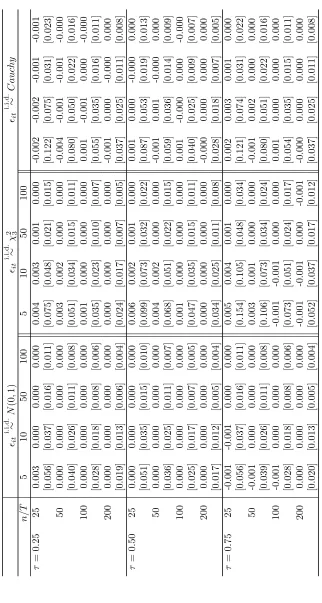
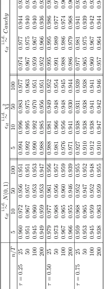
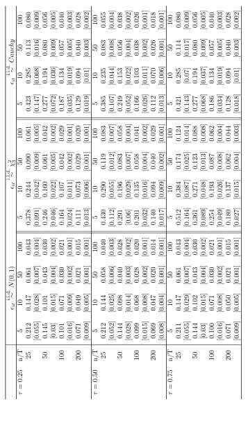
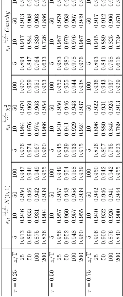
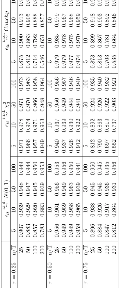
Tables 1, 4 and 7 report the bias and the standard deviation of the FE-QR

estima-tor. Tables 2, 5 and 8 report the average of the estimated standard error (together with

its standard deviation) described in Proposition 3.1. Finally, the empirical coverage

probability of the asymptotic Gaussian confidence interval at the 95% nominal level

is constructed using this estimated standard error (tables 3, 6 and 9). The empirical

coverage probability is also computed. The number of Monte Carlo repetitions is 5000

4.1

Bias

The performance of the FE-QR estimator is evaluated first by its bias. Tables 1, 4 and

7 report the results for the location shift and location-scale shift (γ = 0.5,1) models,

respectively. For the median, the results are in line with those of Koenker (2004), where

in both models the FE-QR estimator has small bias and standard deviation in small

samples. However, there are noticeable differences for the first and third quartiles.

In the location shift model, the bias is small in every case and the standard errors

decrease monotonically as either n or T increases. In the location-scale shift model,

however, both bias and standard errors are large for small T. In particular, the bias

is considerable in the Cauchy and χ2

3 case (in the latter for the third quartile) and

T = 5,10. Moreover, the bias is much larger for the γ = 1 case than for γ = 0.5.9

These results suggest that the FE-QR estimator performs well in small samples for

the location shift model but may have a large bias for the location-scale shift model

where the quantile of interest is evaluated at an associated low density (i.e., F = χ2 3

and τ = 0.75 case) when T is small. Overall, these simulations confirm that the bias

exists for small T and does not depend on n.

4.2

Inference

To study the inference procedure based on the FE-QR estimator, we first compute

the estimated standard error.10 _{The results are reported in tables 2, 5 and 8 for the}

location shift and location-scale shift (γ = 0.5,1) cases, respectively. We also report

the sample standard deviation of the estimator based on the Monte Carlo repetitions

By comparing table 2 with 1, 5 with 4 and 8 with 7, we may see that the estimated

standard error approximates very closely the truth. Second, we calculate the empirical

coverage probability of the asymptotic Gaussian confidence interval at the 95% nominal

level. In this case, the greater distortions appear in the location-scale shift case for

largen/T, and in particular for theχ2

3 case andτ = 0.75. The distortion is very severe

for T = 5,10 and n = 200 for all distributions, despite the fact that the estimated

standard error approximate well the truth. This possibly reflects that the variance of

the FE-QR estimator decreases when nT increases while the bias decreases when T

increases but is independent of n, so that the centering of the confidence interval will

be severely distorted when n/T is large.

9_{Although not reported, we have also performed the same experiments forγ = 0.2. In this case}

the bias is smaller than forγ= 0.5.

10_{For estimation of the asymptotic covariance matrix, we use the Gaussian kernel and the default}

5

Extension: dynamic case

We now extend the asymptotic results in Section 3 to the dynamic case where we

allow for dependence across time while maintaining independence across individuals.

We make the following assumptions in this case.

(D1) {(yit,xit), t ≥ 1} is stationary and β-mixing for each fixed i, and independent

across i. Let βi(j) denote the β-mixing coefficients of {(yit,xit), t ≥ 1}. Then,

there exist constants a ∈ (0,1) and B > 0 such that sup_i≥1βi(j) ≤ Baj for all

j ≥1.

(D2) Let fi,j(u1, u1+j|x1,x1+j) denote the conditional density of (ui1, ui,1+j) given

(xi1,xi,1+j) = (x1,x1+j). There exists a constantCf′ >0 such thatfi,j(u1, u1+j|x1,x1+j)≤

C_f′ uniformly over (u1, u1+j,x1,x1+j) for all i≥1 andj ≥1.

(D3) Let ˜Vnidenote the covariance matrix of the termT−1/2

∑T

t=1{τ−I(uit ≤0)}(xit−

γit). Then, the limit ˜V :=n−1

∑n

i=1V˜ni exists and is nonsingular.

Condition (D1) is similar to Condition 1 of Hahn and Kuersteiner (2004). Condition

(D2) imposes new restrictions on the conditional densities. Note that in Condition (D3)

now ˜Vni is now a long run covariance matrix.

The next theorem shows that similar asymptotic results to those in Section 3 are

obtained for the dependent case. The proof is given in the Appendix.

Theorem 5.1. Assume conditions (D1)-(D3), (A3) and (B1)-(B3). Then, ( ˆα,βˆ) is

weakly consistent provided that (logn)2/T →0. If (logn)2/T →0 but T grows at most polynomially in n, then βˆ admits the expansion (3.2). If moreover n2_(logn)3_/T →_0,

then we have √nT( ˆβ−β0) d

→N(0,Γ−1_V˜Γ−1_).

In proving Theorem 5.1, we need some extensions of empirical process inequalities to

β-mixing sequences, which we believe is a nontrivial task. We develop those extensions

in Appendix C, which are useful in other contexts such as asymptotic analysis of sieve

estimation for β-mixing sequences.

6

Discussion

In this paper, we have studied the asymptotic properties of the FE-QR estimator. The

results found in this paper show that the asymptotic theory for panel models with

non-differentiable objective functions, as in the QR case, should be analyzed carefully.

the sequential asymptotics as long as n/T goes to zero, as is well recognized in the

literature. However, this paper draws a caution that such a result may not directly

apply to the QR case.

There remain several issues to be investigated.

It is an open question whether the convergence rate of the remainder term in (3.2)

can be improved to Op(T−1). It should be pointed out that although the rate of the

remainder term derived in this paper is the best one that we could achieve at this point,

there might be a room for improvement on the rate, which means that our condition

for the asymptotic normality is only a sufficient one. However, although we could not

formally show in this paper, we conjecture that n/T → 0 is a sufficient condition to asymptotic normality of QR panel data. Kato and Galvao (2010) used a smoothed

version of the FE-QR estimator to derive the asymptotic bias of the estimator when

n/T → ρ > 0. Thus, the smoothed estimator is unbiased for n/T → 0. However, it is important to note that the derivation makes use of the smoothness of the objective

and the score functions, which is not applicable to this paper. The challenge in the

present context is that higher order expansions for the standard QR is a very difficult

subject.

Since there is a large literature on analytical bias correction for large panel data,

one could wonder about deriving the asymptotic bias in the present context of FE-QR

estimation. There are at least two important reasons to explain the degree of difficulty

in the FE-QR case. First, the rate Op{(T /logn)−3/4} in the Bahadur representation

in Theorem 3.2 comes from the rate of the score terms, as defined in the proof of

Theorem 3.2. Unfortunately, a direct expansion of these terms with respect to ( ˆα,βˆ)

and the simple evaluation of the mean and variance is not feasible.11 _{It is important}

to note that for each i, the convergence rate of ( ˆαi,βˆ) is dominated by ˆαi, and thus is

at most T−1/2_{. However, because of the non-smoothness of the indicator function, the}

evaluation of these terms based on some moment inequalities for empirical processes

(such as Proposition B.1) leads to the rate Op{max1≤i≤n|αˆi −αi0|3/2}, which turns

out to beOp(T−3/4) (logn term is ignored for simplicity). Thus, a more refined result

(such as a bias result) could be obtained if one could establish the probability limits of

these terms (scaled by a suitable term), which is thought to be a quite challenging task

and is not solved in this paper.12 _{Secondly, there is another difficulty to obtain a bias}

result to the FE-QR estimator. This is related to indeterminateness of the higher order

11_{A way to deal with such terms is to consider them as empirical processes indexed by (α,β), and}

establish the rates by using the preliminary rates of ( ˆα,βˆ). This is what the present proof does.

12_{To obtain a bias result, establishing the exact probability limits of these terms would be essential,}

because the corresponding terms in the standard smooth case contribute to the bias of the resulting

behavior of quantile regression estimators. Consider, for illustrative purposes, a sample

τ-quantile of uniform random variablesu1, . . . , unon [0,1] whereτ ∈(0,1) is fixed and

nτ is integer. Let u(1) <· · ·< u(n) denote the order statistics of u1, . . . , un. Then, the

sampleτ-quantile is usually given byu(nτ). However, if we view of the sample quantile

as a solution to the QR minimization problem, it can be any value in [u(nτ), u(nτ+1)], of

which the mean length is of order n−1_{. This means that the higher order behavior of}

the sampleτ-quantile atn−1 _{rate is not fully determined if we take the sample quantile}

as a solution to the QR minimization problem. Since the asymptotic bias of the general

fixed effect estimator depends on the higher order behavior of the estimators of the

individual parameters atT−1 rate, this indeterminateness would be another challenge

to obtain a bias result to the FE-QR estimator.

A

Proofs

A.1

Proof of Theorem 3.1

PutMni(αi,β) := T−1

∑T

t=1ρτ(yit−αi−x′itβ) and ∆ni(αi,β) :=Mni(αi,β)−Mni(αi0,β0).

For each δ > 0, define Bi(δ) := {(α,β) : |α−αi0|+∥β−β0∥1 ≤ δ} and ∂Bi(δ) :=

{(α,β) :|α−αi0|+∥β−β0∥1 =δ}.

Proof of Theorem 3.1. We divide the proof into two steps.

Step 1. We first prove ˆβ →p β0. Fix any δ > 0. For each (αi,β) ∈/ Bi(δ), define

˜

αi =riαi+ (1−ri)αi0, β˜i =riβ+ (1−ri)β0, where ri =δ/(|αi −αi0|+∥β−β0∥1).

Note that ri ∈ (0,1) and ( ˜αi,β˜i) ∈ ∂Bi(δ). Because of the convexity of the objective

function, we have

ri{Mni(αi,β)−Mni(αi0,β0)} ≥Mni( ˜αi,β˜)−Mni(αi0,β0)

={E[∆ni( ˜αi,β˜i)]}+{∆ni( ˜αi,β˜i)−E[∆ni( ˜αi,β˜i)]}. (A.1)

Use the identity of Knight (1998) to obtain

E[∆ni(αi,β)] = E

[∫ (αi−αi0)+x′i1(˛−˛0)

0

{Fi(s|xi1)−τ}ds

]

.

From condition (A3), the first term on the right side of equation (A.1) is greater than

or equal to ϵδ for all 1≤i≤n. Thus, by (A.1), we obtain the inclusion relation

{

∥_βˆ_−β

0∥1 > δ

}

⊂ {Mni(αi,β)≤Mni(αi0,β0), 1≤ ∃i≤n, ∃(αi,β)∈/ Bi(δ)}

⊂ {

max

1≤i≤n_(α sup

i,˛)∈Bi(δ)

|∆ni(αi,β)−E[∆ni(αi,β)]| ≥ϵδ

}

The first inclusion follows from the following argument. Suppose that ∥βˆ−β0∥1 > δ.

Then, ( ˆαi,βˆ)∈/ Bi(δ) for all 1≤i≤n. IfMni( ˆαi,βˆ)>Mni(αi0,β0) for all 1≤i≤n,

then∑n_i=1Mni( ˆαi,βˆ)>

∑n

i=1Mni(αi0,β0), which however contradicts the definition of

( ˆα,βˆ). Thus, Mni( ˆαi,βˆ) ≤ Mni(αi0,β0) for some 1 ≤ i ≤ n, which leads to the first

inclusion.

Therefore, it suffices to show that for every ϵ >0,

lim

n→∞P

{

max

1≤i≤n_(α sup

i,˛)∈Bi(δ)

|∆ni(αi,β)−E[∆ni(αi,β)]|> ϵ

}

= 0. (A.2)

[Recall thatT =Tn is indexed by n, andn → ∞automatically means thatT =Tn →

∞.]

Because of the union bound, it suffices to prove that for every ϵ >0,

max

1≤i≤nP

{

sup

(α,˛)∈Bi(δ)

|∆ni(α,β)−E[∆ni(α,β)]|> ϵ

}

=o(n−1). (A.3)

We follow the proof of Fernandez-Val (2005, Lemma 7) to show (A.3). Without loss

of generality, we may assume that αi0 = 0 and β0 = 0. Then, Bi(δ) is independent

of i and write Bi(δ) =B(δ) for simplicity. Putgα,˛(u,x) :=ρτ(u−α−x′β)−ρτ(u).

Observe that |gα,˛(u,x)−gα,¯˛¯(u,x)| ≤ C(1 +∥x∥1)(|α−α¯|+∥β −β¯∥1) for some

universal constant C > 0. Put L(x) := C(1 + ∥x∥1) and κ := supi≥1E[L(xi1)].

SinceB(δ) is a compact subset ofRp+1_{, there existK ℓ}

1-balls with centers (α(j),β(j)),

j = 1, . . . , K and radius ϵ/(7κ) such that the collection of these balls covers B(δ).

Note that K is independent of i and can be chosen such that K = K(ϵ) = O(ϵ−p−1)

as ϵ → 0. Now, for each (α,β) ∈ B(δ), there is a j ∈ {1, . . . , K} such that

|gα,˛(u,x)−gα(j)_,˛(j)(u,x)| ≤L(x)ϵ/(7κ), which leads to |∆_ni(α,β)−E[∆_ni(α,β)]| ≤

|∆ni(α(j),β(j))−E[∆ni(α(j),β(j))]|+{ϵ/(7κ)} · |T−1

∑T

t=1{L(xit)−E[L(xi1)]}|+ 2ϵ/7.

Therefore, we have

P

{

sup

(α,˛)∈B(δ)

|∆ni(α,β)−E[∆ni(α,β)]|> ϵ

}

≤

K

∑

j=1

P

{

|∆ni(α(j),β(j))−E[∆ni(α(j),β(j))]|>

ϵ 3

}

+ P

{

1 T

¯¯ ¯¯ ¯

T

∑

t=1

{L(xit)−E[L(xi1)]}

¯¯ ¯¯ ¯>

7κ 3

}

. (A.4)

Since sup_i≥1E[L2s(xi1)] < ∞, application of the Marcinkiewicz-Zygmund inequality

(see Corollary 2 in Chow and Teicher, 1997, p. 387) implies that both terms on the

T, they areo(n−1_{), leading to (A.3).}

Step 2. Next, we shall show that max1≤i≤n|αˆi − αi0|

p

→ 0. Recall that ˆαi =

arg minαMni(α,βˆ). Fix any δ > 0. For each αi ∈ R such that |αi −αi0| > δ,

de-fine ˜αi = riαi + (1−ri)αi0, where ri = δ/|αi −αi0|. Because of the convexity of the

objective function, we have

ri{Mni(αi,βˆ)−Mni(αi0,βˆ)} ≥Mni( ˜αi,βˆ)−Mni(αi0,βˆ)

=Mni( ˜αi,βˆ)−Mni(αi0,β0)− {Mni(αi0,βˆ)−Mni(αi0,β0)}

={∆ni( ˜αi,βˆ)−E[∆ni( ˜αi,β)]|_{˛= ˆ˛}} − {∆ni(α0i,βˆ)−E[∆ni(α0i,β)]|_{˛= ˆ˛}}

+ E[∆ni( ˜αi,β0)] +{E[∆ni( ˜αi,β)]|˛= ˆ˛−E[∆ni( ˜αi,β0)]}+ E[∆ni(α0i,β)]|˛= ˆ˛. It is seen from condition (A3) that the third term on the right side is greater than or

equal to ϵδ. Thus, we obtain the inclusion relation

{|αˆi−αi0|> δ, 1≤ ∃i≤n}

⊂ {Mni(αi,βˆ)≤Mni(αi0,βˆ), 1≤ ∃i≤n, ∃αi ∈Rs.t. |αi−αi0|> δ}

⊂ {

max

1≤i≤n_|α−sup_α

i0|≤δ

|∆ni(α,βˆ)−E[∆ni(α,β)]|˛= ˆ˛| ≥ ϵδ

4

}

∪ {

max

1≤i≤n_|α−sup_α

i0|≤δ

||E[∆ni(α,β)]|˛= ˆ˛ −E[∆ni(α,β0)]| ≥

ϵδ

4

}

=:A1n∪A2n.

Since ˆβ is consistent by Step 1, and especially ˆβ = Op(1), by (A.2), it is shown that

P(A1n)→0. Finally, since

|E[∆ni(α,β)]−E[∆ni(α,β0)]| ≤2E[∥xi1∥]∥β−β0∥,

and sup_i≥1E[∥xi1∥]≤1+supi≥1E[∥xi1∥2s]<∞, consistency of ˆβimplies that P(A2n)→

0. Therefore, we complete the proof.

Remark A.1. If sup_i≥1∥xi1∥ ≤ M (a.s.) for some constant M, we may take L(x)≡

C(1 +M) and the second term on the right side of (A.4) will vanish. In this case,

we can apply Hoeffding’s inequality to the first term on the right side of (A.4) and

the probability in (A.3) is bounded byDexp(−DT) for some positive constantDthat depends on ϵ but not on i. Therefore, the conclusion of Theorem 3.1 holds when

A.2

Proof of Theorem 3.2

Define

H(1)

ni(αi,β) :=

1 T

T

∑

t=1

{τ −I(yit ≤αi+x′itβ)},

H_ni(1)(αi,β) := E[Hni(1)(αi,β)] = E[{τ −Fi(αi−αi0+x′i1(β−β0)|xi1)}],

H(2)

n (α,β) :=

1 nT

n

∑

i=1 T

∑

t=1

{τ−I(yit ≤αi+x′itβ)}xit,

H_n(2)(α,β) := E[H(2)_n (α,β)] = 1 n

n

∑

i=1

E[{τ−Fi(αi−αi0+xi1′ (β−β0)|xi1)}xi1].

Note that H(1)_ni(αi,β) depends on n since T does. The (n+p) dimensional vector of

functions [H(1)_n1(α1,β), . . . ,H (1)

nn(αn,β),H (2)′

n (α,β)]′ are called the scores for problem

(2.2).

Before starting the proof, we introduce some notation used in empirical process

theory. LetF be a class of measurable functions on a measurable space (S,S). For a processZ(f) defined onF,∥Z(f)∥_F := sup_f∈F|Z(f)|. For a probability measureQon (S,S) andϵ >0, letN(F, L2(Q), ϵ) denote theϵ-covering number ofF with respect to

the L2(Q) norm ∥ · ∥L2(Q). For the definition of a Vapnik- ˇCervonenkis (VC) subgraph

class, we refer to van der Vaart and Wellner (1996), Section 2.6. For a, b∈R, we use the notationa∨b:= max{a, b}.

Proof of Theorem 3.2. Recall first that by Theorem 3.1, under the present conditions, ( ˆα,βˆ)) is weakly consistent. We divide the proof into several steps.

Step 1 (Asymptotic representation). We shall show that

ˆ

β−β0+op(∥βˆ−β0∥) = Γ−n1{−n− 1∑n

i=1H (1)

ni(αi0,β0)γi+H(2)n (α0,β0)}

−Γ−_n1[n−1∑n_i=1γi{H (1)

ni( ˆαi,βˆ)−H (1)

ni ( ˆαi,βˆ)−H (1)

ni(αi0,β0)}]

+ Γ−_n1{H(2)_n ( ˆα,βˆ)−H_n(2)( ˆα,βˆ)−H_n(2)(α0,β0)}

+Op{T−1 ∨ max

1≤i≤n|αˆi−αi0| 2_}

. (A.5)

Because of the computational property of the QR estimator (see equation (3.10) of

Gutenbrunner and Jureckova, 1992), it is shown that max1≤i≤n|H (1)

ni( ˆαi,βˆ)|=Op(T−1).

Thus, uniformly over 1≤i≤n, we have Op(T−1) = H

(1)

ni(αi0,β0) +H (1)

ni ( ˆαi,βˆ) +{H (1)

ni( ˆαi,βˆ)−H (1)

ni ( ˆαi,βˆ)−H (1)

ni(αi0,β0)}.

ExpandingH_ni(1)( ˆαi,βˆ) around (αi0,β0), we have

ˆ

αi−αi0 ={fi(0)}−1H (1)

ni(αi0,β0)−γi′( ˆβ−β0)

+{fi(0)}−1{H (1)

ni( ˆαi,βˆ)−H (1)

ni ( ˆαi,βˆ)−H (1)

where max1≤i≤n|rˆni|=Op{T−1∨max1≤i≤n|αˆi−αi0|2∨ ∥βˆ−β0∥2}.

Similarly, the computational property of the QR estimator implies that∥H(2)n ( ˆα,βˆ)∥=

Op{T−1max1≤i≤n,1≤t≤T ∥xit∥}=Op(T−1), from which we have

Op(T−1) =H(2)n (α0,β0)+Hn(2)( ˆα,βˆ)+{H (2)

n ( ˆα,βˆ)−H (2)

n ( ˆα,βˆ)−H (2)

n (α0,β0)}. (A.7)

Use Taylor’s theorem to obtain

H_n(2)( ˆα,βˆ) =−1 n

n

∑

i=1

E[fi(0|xi1)xi1]( ˆαi−αi0)−

{

1 n

n

∑

i=1

E[fi(0|xi1)xi1x′i1]

}

( ˆβ−β0)

+op(∥βˆ−β0∥) +Op

{

max

1≤i≤n|αˆi−αi0| 2

}

. (A.8)

Plugging (A.6) into (A.8) leads to

H_n(2)( ˆα,βˆ) =−1 n

n

∑

i=1

H(1)

ni(αi0,β0)γi−Γn( ˆβ−β0)

− 1

n

n

∑

i=1

γi{H(1)ni( ˆαi,βˆ)−Hni(1)( ˆαi,βˆ)−H(1)ni(αi0,β0)}

+op(∥βˆ−β0∥) +Op

{

T−1∨ max

1≤i≤n|αˆi−αi0| 2

}

. (A.9)

Combining (A.7) and (A.9) yields the desired representation. The remaining steps are

devoted to determining the order of the remainder terms in (A.5).

Step 2 (Rates of the remainder terms). Takeδn →0 such that max1≤i≤n|αˆi−αi0| ∨

∥_βˆ_{−β0∥=Op(δn). We shall show that}

∥n−1∑n_i=1γi{H (1)

ni( ˆαi,βˆ)−H (1)

ni ( ˆαi,βˆ)−H (1)

ni(αi0,β0)}∥=Op(dn), (A.10)

∥H(2)

n ( ˆα,βˆ)−H (2)

n ( ˆα,βˆ)−H (2)

n (α0,β0)∥=Op(dn). (A.11)

where dn:=T−1|logδn| ∨T−1/2δ 1/2

n |logδn|1/2.

We only prove (A.10) since the proof of (A.11) is analogous.13 _{Without loss of}

generality, we may assume that αi0 = 0 and β0 = 0. Put gα,˛(u,x) := I(u ≤ α+

x′β)− I(u ≤ 0), Gδ := {gα,˛ : |α| ≤ δ,∥β∥ ≤ δ} and ξit := (uit,xit). Since γi is

bounded over i, it suffices to show that

max

1≤i≤nE

 °°°°

°

T

∑

t=1

{g(ξit)−E[g(ξi1)]}

°° °° °

Gδn



=O(dnT). (A.12)

13_{Although the present proof requires x}

i1 to be bounded, it is possible to use Theorem 2.14.1 of

van der Vaart and Wellner (1996) to show (A.11), which only requires that sup_i≥1E[∥xi1∥2] <∞.

To this end, we apply Proposition B.1 to the class of functions ˜Gi,δn :={g−E[g(ξi1)] :

g ∈ Gδn}. Observe that ˜Gi,δn is pointwise measurable and each element of ˜Gi,δn is

bounded by 2. Because of Lemmas 2.6.15 and 2.6.18 of van der Vaart and Wellner

(1996), the class G_∞ := {gα,˛ : α ∈ R,β ∈ Rp} is a VC subgraph class. Thus, by Theorem 2.6.7 of van der Vaart and Wellner (1996), the fact that ˜Gi,δn ⊂ {g −

E[g(ξi1)] : g ∈ G∞}, and a simple estimate of covering numbers, there exist constants

A≥3√e and v ≥1 independent of i and n such thatN( ˜Gi,δn, L2(Q),2ϵ)≤(A/ϵ)

v _for

every 0 < ϵ < 1 and every probability measure Q on Rp+1_{. Combining the fact that}

E[gα,˛(ξi1)2] = E[|Fi(α+x′i1β|xi1)−Fi(0|xi1)|] ≤ Cf(|α|+M∥β∥), one can see that

˜

Gi,δn satisfies all the conditions of Proposition B.1 withU = 2 and σ

2 _=C

f(1 +M)δn,

and the constants A and v are independent of iand n. This implies that the left side

of (A.12) is O(dnT).

Step 3 (Preliminary convergence rates). We shall show that

max

1≤i≤n|αˆi−αi0|=Op{(T /logn)

−1/2_{}, ∥βˆ−β}

0∥=op{(T /logn)−1/2}.

We first show that max1≤i≤n|αˆi−αi0|=Op{(T /logn)−1/2}. Because of consistency

of ( ˆα,βˆ) and the result given in Step 2, the second and third terms on the right side

of (A.5) is op(T−1/2), which implies that

∥_βˆ_−β

0∥=Op{max

1≤i≤n|αˆi−αi0| 2_}+o

p(T−1/2). (A.13)

Thus, by (A.6), max1≤i≤n|αˆi−αi0| is bounded by

const.×

{

max

1≤i≤n|H (1)

ni(αi0,β0)|+ max 1≤i≤n|H

(1)

ni( ˆαi,βˆ)−H (1)

ni ( ˆαi,βˆ)−H (1)

ni(αi0,β0)|

}

+op(T−1/2),

with probability approaching one.

First, observe that for any K >0,

P

{

max

1≤i≤n|H (1)

ni(αi0,β0)|>(T /logn)−1/2K

} ≤

n

∑

i=1

P

{ |H(1)

ni(αi0,β0)|>(T /logn)−1/2K

}

,

and the right side is bounded by 2n1−K2/2 by Hoeffding’s inequality. This implies that

max1≤i≤n|H (1)

ni(αi0,β0)|=Op{(T /logn)−1/2}.

We next show that

max

1≤i≤n|H (1)

ni( ˆαi,βˆ)−H (1)

ni ( ˆαi,βˆ)−H (1)

ni(αi0,β0)|=op{(T /logn)−1/2},

which leads to the first result. Without loss of generality, as before, we may assume