On the modified monotonic loading concept for the calculation of the cyclic j-integral

1

On The Modified Monotonic Loading

Concept for the Calculation of the

Cyclic J-Integral

Ross Beesley

Department of Mechanical & Aerospace Engineering, University of Strathclyde, Glasgow, G1 1XJ, UK

Haofeng Chen1

Department of Mechanical & Aerospace Engineering, University of Strathclyde, Glasgow, G1 1XJ, UK

Martin Hughes

Siemens Industrial Turbomachinery Ltd, Waterside South, Lincoln, LN5 7FD

ABSTRACT

This paper investigates an approach for calculating the cyclic J-Integral through a new industrial

application. A previously proposed method is investigated further with the extension of this technique

through a new application of a practical 3D notched component containing a semi-elliptical surface crack.

Current methods of calculating the cyclic J-Integral are identified and their limitations discussed. A

modified monotonic loading concept is adapted to calculate the cyclic J-integral of this 3D Semi Elliptical

Surface Crack under cyclic loading conditions. Both the finite element method (FEM) and the Extended

Finite Element Method (XFEM) are discussed as possible methods of calculating the cyclic J-Integral in this

investigation. Different loading conditions including uniaxial tension and out of plane shear are applied,

and the relationships between the applied loads and the cyclic J-integral are established. In addition, the

variations of the cyclic J-integral along the crack front are investigated. This allows the critical load that

can be applied before crack propagation occurs to be determined as well as the identification of the critical

crack direction once propagation does occur.

These calculations display the applicability of the method to practical examples and illustrate an accurate

method of estimating the cyclic J-integral.

Keywords: crack, J-integral, cyclic J-integral, fracture mechanics, FEA, XFEM

1 _{Corresponding author}

2 NOMENCLATURE

A Dowling and Begley Fatigue Law Constant

C Paris' Law Constant

da Change in crack length

dN Change in number of cycles

J J-Integral

ΔJ Cyclic J-Integral

Jmax J-Integral at maximum cyclic load

Jmin J-Integral at minimum cyclic load

K Stress Intensity Factor

ΔK Stress Intensity Factor range

Kmax Stress Intensity Factor at maximum cyclic load

Kmin Stress Intensity Factor at minimum cyclic load

m Paris' Law Constant

MPa Mega Pascals

N Newtons

ε Strain

3 1 INTRODUCTION

Fracture mechanics regards the initiation and propagation of cracks. The impact of material fracture varies depending on the specific application but the results can be catastrophic. Therefore, gaining an understanding of fracture and failure is very important. The ability to predict when a crack will initiate and fail, and thus the resulting fatigue life of the component must be understood to ensure the safe design and utilisation of structural components. Fracture mechanics provides generalized techniques that are widely applied to a number of different industries and applications. For this reason, this field of study has attracted a large number of researchers [1-6].

Stress raisers are of particular importance when considering engineering components. Design features such as notches or sharp corners, and even minor defects such as scratches and corrosion can introduce stress raisers which reduce the critical stress at which crack initiation can occur. Such features can limit the fatigue life since failure can occur at a reduced load or fewer loading cycles. The stress intensity factor (SIF), is a measure of the stress conditions near a crack tip and can be used to predict stress and fracture behaviour under different loading conditions. Extensive experimental testing has permitted the development of a set of standardized equations for calculating the stress intensity factor for a number of different crack and model geometries.

4 cyclic fatigue are investigated through the application of techniques on an industrial test specimen.

1.1 Objectives

The overarching aim of this investigation is to assess the suitability of an extended

monotonic analysis for approximating the cyclic J-integral (ΔJ). Initially, the limitations with the current methods of determining the cyclic J-Integral will be identified. The suitability of the proposed Modified Monotonic Loading (MML) concept will then be assessed. Finally, this technique will be applied to an industrial test specimen in order to calculate the cyclic J-Integral and its variation with increasing load and crack front location. This paper is organised as follows:

Section 2 discusses the background theory of numerical methods that exist for addressing crack modelling. In Section 3, finite element methods are introduced and the proposed concept for calculating the ΔJ will be discussed. Section 4 presents the model specific to this application and the associated material and loading properties defined. The investigation continues with Section 5 which presents the obtained results for the validation of the MML technique as well as the calculated cyclic J-Integral variation with increasing load and crack location.

2 THEORETICAL BACKGROUND 2.1 Contour Integrals

5 2.2 Fatigue Life

In order to calculate the fatigue life under Linear Elastic Fracture Mechanics (LEFM), the stress intensity factor, K, is required. The SIF is a function of stress and crack length. Under cyclic loading conditions, the SIF range between maximum and minimum loading can be used to predict fatigue life through Paris’ Law*15] as shown in Eq 1.

(1)

Where a is crack length, N is number of cycles, ΔK=Kmax-Kmin is the stress intensity factor

range and C and m are constants. This relationship holds for LEFM properties, however it does not apply to Elastic-Plastic Fracture Mechanics (EPFM) properties since the relationship becomes less accurate as plasticity levels increase. Therefore, a new parameter is required to allow a similar approach for calculating the fatigue life of elastic-plastic materials. A suitable alternative is the J-Integral, which represents a method of calculating the strain energy release rate per unit area of a fracture surface. The J-Integral offers an EPFM equivalent to the SIF for LEFM. Calculating the J-Integral under monotonic loading conditions is relatively simple. It is done routinely and has proven itself to be a good method of modelling crack behaviour. However, difficulties arise when implementing cyclic loading conditions.

The cyclic J-Integral, is a function of the stress and strain range, Δσ and Δε and as a result, unlike the cyclic stress intensity factor, is not simply equal to Jmax-Jmin and

therefore . For this reason, calculating the cyclic J-Integral is inherently

more difficult than for monotonic loading and no standard techniques have yet been developed to determine the cyclic J-integral. In order to determine the EPFM fatigue life, the J-Integral must be extended to allow for cyclic loading conditions, much like the SIF range is used in LEFM cyclic fatigue.

6 dominated by the elastic component and so the linear elastic based strain energy release rate is sufficient for calculating J. However, when the effect of the plastic zone becomes more substantial, this linear elastic approximation is no longer valid. Therefore, since the J-Integral can be used to determine the fatigue life, a reliable method of its calculation is vitally important.

The cyclic J-Integral was first proposed and implemented by Dowling and Begley[17]. A power law behaviour, similar to that of the Paris equation was developed and so the fatigue crack growth rate of cyclic loading EPFM can be written as:

( ) (2)

where A and m are material constants.

2.3 Limitations of Existing Technologies

The GE/EPRI[18] and Reference Stress Method (RSM)[19] offer simplified methods of approximating the cyclic J-Integral. However, due to the nature of these methods they exhibit considerable limitations and thus produce overly conservative results. Both of these methods are based on the limit load analysis and as such do not consider the crack geometry, meaning that they are unable to assess three dimensional detail. Consequently, the ΔJ variation along the crack front cannot be determined and thus valuable crack propagation information is neglected. In addition, these methods are suitable for a number of documented test cases such as compact tension specimens, however, difficulties arise when applying these methods to bespoke specimens.

These limitations provide great approximations in the calculation of the cyclic J-Integral, significantly reducing the accuracy of the results. For these reasons, these methods are not considered appropriate for complex 3D industrial applications.

7 would require extensive and very time consuming post processing of the analysis history data. Manually calculating in this way is therefore not feasible and so a more automated method is required if the cyclic J-Integral is to be viable fatigue life parameter.

2.4 Crack Modelling

Simulating a 3D surface crack is much more complicated than a 2D crack. The variation of ΔK and ΔJ along the crack front is dependent on the type and magnitude of the applied loading and as a result will vary depending upon the location along the 3D surface crack front. Different locations will result in different values of ΔK and ΔJ and will thus affect the crack propagation direction. It is therefore vitally important to simulate the ΔJ with a high level of detail under different loading conditions in order to gain an understanding of the crack behaviour and thus predict its propagation.

3 NUMERICAL METHOD

Modelling simplified models such as infinite plates and blocks can provide valuable insight into crack behaviour. However, these large simplifications can overlook the complexities of real life applications that are found in industry. Therefore, increasing the model complexity makes computational models more akin to industrial applications and thus the results can offer more value than that of greatly simplified cases. This provides reason for modelling a complex geometry test specimen in this investigation.

3.1 Finite Element Analysis (FEA) Crack Simulation

FEA allows the modelling of cracks and the calculation of their associated parameters such as SIF and J-Integral. Within ABAQUS, cracks can either be modelled using the traditional Finite Element Method (FEM) or the Extended Finite Element Method (XFEM) [20].

8 separate. This method currently only offers modelling of stationary cracks, meaning that propagation cannot automatically be modelled unlike XFEM. Within FEM, mesh quality around the crack tip is critical and must be refined sufficiently to allow for acceptable accuracy which increases the computational modelling and analysis effort.

3.2 Extended Finite Element Method (XFEM)

The extended finite element method is capable of modelling mesh independent cracking, meaning that crack initiation and propagation can be modeled without prior definition. A propagating crack does not need to adhere to element boundaries unlike the traditional finite element method (FEM). This reduces the importance of mesh refinement in the region of the crack front. XFEM can model stationary or propagating cracks, however ABAQUS is currently only capable of determining crack parameters such as SIF and J-Integral for stationary cracks. This method is still in its infancy but it shows a great deal of potential. It provides a simple method of modeling complex crack geometries without the need for extensive mesh refinement which can be very computationally expensive both in implementation and analysis. This method is capable of calculating contour integrals such as the SIF and J-Integral, however, when a high level of geometrical detail is introduced, the accuracy of contour integration close to the crack tip is compromised. For this reason, XFEM will not be used as a technique for calculating contour integrals in this investigation and traditional FEM will be used instead.

3.3 Modified Monotonic Loading (MML) Concept

A concept has been proposed which provides a reasonable approximation for the calculation of the cyclic J-Integral which addresses the known issues in the existing technologies. This can be achieved through modification of a monotonic loading analysis by replacing σywith 2σy and replacing the cyclic load range with a single monotonic load

9 Modified Monotonic Loading (MML) concept. This follows on from the work of Chen and Chen[21]. It was discovered that in an un-cracked body subjected to variable loading conditions, the differences between this MML concept and the equivalent cyclic analysis were relatively small. Their work indicated the potential for this technique as a method of determining the cyclic J-Integral. In this investigation, this MML concept will be

investigated and tested further on an industrial test specimen. Rice[3] originally defined the J-Integral in two dimensions as:

∫ ( ) (3)

Where T is the traction vector, u is the displacement vector, ds is an element of arc length along the contour path, Γ, and W is the strain energy density which is given by:

∫ (4)

Where ε is an infinitesimal strain tensor.

Tanaka [22] later extended this for cyclic loading between two states, i and j, as:

∫ ( ) (5)

Altering the terminology to match Rice’s original equation, allows it to be represented as:

∫ ( ) (6)

Where ΔW is the strain energy density range between two states, i and j, which is a function of the stress and strain range and is given by:

∫( ) ( )

( ) (7)

Where and are the stress and strain tensors respectively and and

denote relative changes between values corresponding to the load change from

one state to another.

10 data from the modified monotonic loading analysis must match the stress range and strain range data from a cyclic loading analysis, Eq. (10) & Eq. (11).

Using this assumption will then allow the determination of the cyclic J-Integral through the MML concept within ABAQUS. Following such a hypothesis, the cyclic J-Integral values under fatigue loading can be assumed to be equal to the J-Integral

values from the Modified Monotonic Loading analysis, Eq. (12). It is assumed that:

( ) (8)

( ) (9)

Therefore, if

(10)

And

(11)

Then,

(12)

Therefore, for a cyclic loading analysis of a particular load range, the cyclic J-Integral can be approximated by performing a Modified Monotonic Loading analysis with a single load equal to the cyclic range.

11 4 NUMERICAL APPLICATION

4.1 Finite Element Model

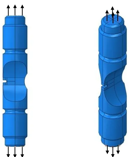
The finite element software package, ABAQUS was used for the computational analyses performed in this investigation. Within ABAQUS, a notched industrial test specimen as presented by Leidermark[23] was modelled with appropriate model

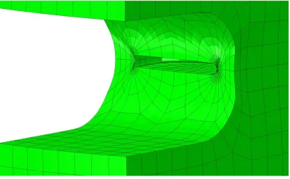
partitioning employed. Fig 1 shows the geometry of the test specimen used in this investigation. This allowed the implementation of a refined mesh around the most critical region of the notch, whilst a more coarse mesh was modelled in the less critical regions. Second order hexahedral elements were implemented in the model with swept elements in the crack front region and structured elements elsewhere.

A 3D elliptical surface crack with a major axis radius of 1mm and a semi-minor axis radius of 0.75mm was modelled with a focused mesh swept along the crack front to allow for improved accuracy. Cyclic and Modified Monotonic Loading analyses were performed and the results of each compared in order to assess the suitability of the method. Once validated, additional MML analyses were performed to calculate the cyclic J-Integral under uniaxial and out of plane shear loading. The finite element mesh of the test specimen is shown in Fig. 2 and a close-up of the opened crack surfaces shown in Fig. 3.

4.2 Material Properties and Loading Conditions

A nickel based super alloy similar to those in turbine applications was used in this investigation. An elastic-perfectly plastic material model was implemented with a Young’s Modulus of 207GPa, Poissons’ Ratio of 0.29 and Yield Stress of 1000MPa. The accuracy of the technique was tested under uniaxial tension and out of plane shear with both cyclic loading and modified monotonic loading conditions. This allowed the accuracy of the technique to be determined when applied to an industrial test specimen under different loading conditions.

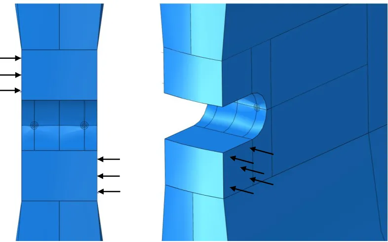
12 zero was applied and for the equivalent Modified Monotonic Loading analysis, a monotonic pressure load of 250MPa was applied. Under out of plane shear loading, pressure forces were applied to the specimen above and below the notch. For the cyclic loading analysis, a cyclic load range of 600MPa with a R-Ratio of zero was applied and for the corresponding MML analysis, a monotonic pressure load of 600MPa was applied.

Diagrams showing the location of the applied forces for uniaxial tension and out of plane shear are shown in Fig. 4 and Fig. 5 respectively.

These analyses were merely comparative in order to visualise the differences between the cyclic loading and MML concept. Following successful validation, additional tensile tests and out of plane shear tests were performed in order to calculate the cyclic J-Integral using the proposed method.

5 RESULTS AND DISCUSSION 5.1 Validation of MML Concept

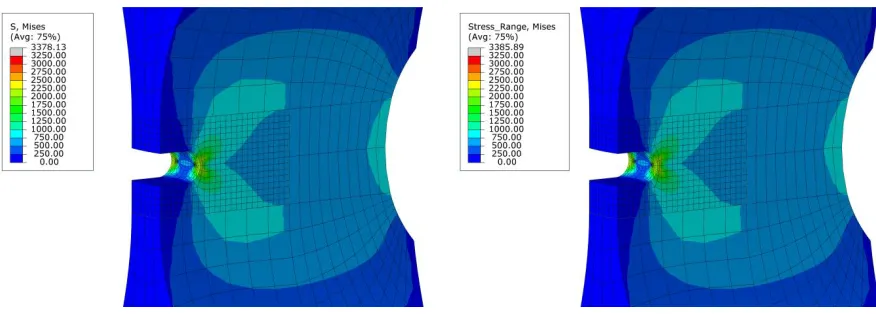
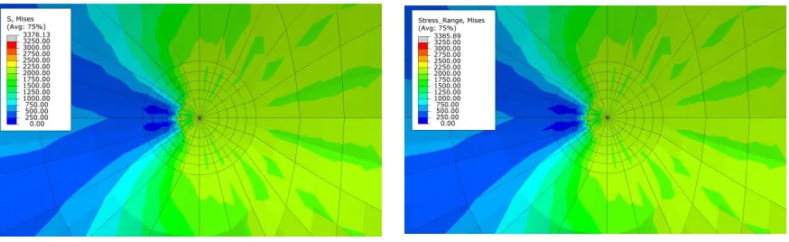
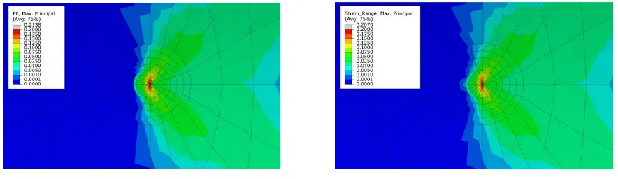
The MML results were compared to the cyclic loading analysis to assess the suitability of the technique as a method of calculating the cyclic J-Integral. The stress range and strain range data from the cyclic loading analysis was compared to the stress and strain data of the MML concept. Fig. 6 to Fig. 9 show Von Mises stress and Von Mises stress range and Maximum Principal strain and Maximum Principal strain range data from the MML and cyclic loading analyses for the uniaxial tension test. Fig. 10 to Fig. 13 show Von Mises stress and Von Mises stress range and Maximum Principal strain and Maximum Principal strain range data from the MML and cyclic loading analyses for the out of plane shear test. From comparing the contour plots of the MML and cyclic analyses, it can be seen that the differences between the two are minimal as the contour plots match very closely. As is assumed in Eq. (9) to Eq. (12), if the stress and strain data of the MML concept matches the stress range and strain range data of the cyclic analysis, then the MML can be assumed to be a reasonable approximation of the cyclic J-Integral.

13 This is believed to be due to crack tip singularities and caused by numerical errors in the finite element calculation. In order to maintain the highest level of accuracy, it is important to greatly refine the mesh in the crack front region. However, due to the complexity of the geometry of the model, the degree to which the mesh can be refined is limited. The aim of this investigation is to provide a direct comparison between the

stress and strain solutions of the MML concept and cyclic analyses under two different loading conditions. Since identical meshes are used in each analysis, the importance of a highly refined mesh in the critical regions is less critical. For this reason, it is believed that this error has little to no effect on the aim of this research and so the meshing rules used in this investigation are believed to be sufficient. However, it is important to consider the effect of the mesh refinement at the crack front when performing detailed analyses for the calculation of the cyclic J-Integral.

This technique means that a simple monotonic analysis is capable of determining the cyclic J-Integral. This offers a quick and computationally inexpensive method of determining the ΔJ, which would otherwise be difficult and time consuming to calculate. From Eq. (2), it can offer an invaluable method of predicting the EPFM fatigue life of a component.

Some minor discrepancies exist between the contour plots of the MML and the cyclic loading analysis, however these differences are small and so the results are believed to be reasonable. It is felt that the speed and ease of implementation and calculation of this technique far outweighs any potential loss in accuracy.

5.2 Determination of cyclic J-Integral using MML

14 crack front showing the node locations and numbers. Node 1 is located at the far left crack edge and Node 25 is located at the far right crack edge when facing the crack opening. These node numbers are referred to in the results in Table 1, Table 2, Fig. 18 and Fig. 19. For each node along the crack front, the ΔJ was calculated at 5 contours encircling the crack front. This is illustrated in Fig. 15. The 5 contours at each node were

averaged to give a single average value at each node along the crack front. This is believed to be accurate since the J-Integral is a path independent parameter[3], meaning that the value is the same, regardless of the path along which it is calculated. Within ABAQUS, numerical errors due to crack tip singularities mean that the values at each contour are not exactly equal, but any differences are very small and so average values are believed to be sufficiently accurate. Values of the cyclic J-Integral at each contour path at each load are shown in Table 3 for uniaxial tension and Table 4 for out of plane shear loading. It can be seen that the first contour is slightly different to the remaining 4 contours, which have close agreement. This demonstrates the differences that occur at the crack tip due to numerical errors are very minor and so the J-Integral can be assumed to be path independent.

The single values at each node were then tabulated and the average and maximum recorded, as well as far left end of crack, centre of crack and far right end of crack, shown in Table 1 for uniaxial tension, and Table 2 for out of plane shear. The J-Integrals provided in Table 1 and Table 2 are obtained by the traditional elastic plastic fracture mechanics FEA using the MML concept. From the original hypothesis, the J integral calculated from the MML concept is assumed to be equal to the cyclic J-Integral of a cyclic loading analysis when the applied load range is equal to the magnitude of the load in the tables. Therefore these presented values can be regarded as the cyclic J-Integral.

15 variation of the ΔJ along the crack front varies widely. Fig. 18 shows this for applied uniaxial tension monotonic loads of 250MPa and 125MPa. A maximum ΔJ value occurs slightly inside from the end of the crack, 3 nodes from each end and a minimum value occurs in the central region of the crack, where it is relatively constant. However the maximum and minimum values differ by a factor of 3. The variation of rate of change of

cyclic J-Integral with increasing load is not linear across the length of the crack. With increasing load, the maximum ΔJ values increase more rapidly and the minimum values increase more slowly relative to the values at the centre of the crack.

Under out of plane shear loading (Fig. 17), it can be seen that the J-Integral relationship with increasing load is very different to that of uniaxial tension. Fig. 19 shows the variation of ΔJ along the crack front under out of plane shear forces of 600MPa and 300MPa. The maximum cyclic J-Integral coincides with the crack left and crack right positions with the crack centre being considerably less. This variation of ΔJ is due to the asymmetry of the loading conditions. This implies that the likeliest point of crack initiation under out of plane shear loading is at each side of the crack. The relationship is much more uniform than that of uniaxial tension with the maximum values occurring at the crack edge. The ΔJ steadily decreases along the crack front to a minimum at the centre with the maximum and minimum values differing by a factor of 5. The rate of change of ΔJ along the crack front is much more uniform than that of uniaxial tension.

6 CONCLUSIONS

16 calculate the cyclic J-Integral to be ascertained. Once validated, additional analyses were performed on the test specimen which allowed the calculation of the cyclic J-Integral. Its variation with increasing load as well as along the crack front was recorded and the following observations have arisen:

1. Under uniaxial tension, the maximum ΔJ occurs slightly inside from the crack edge with the minimum being at the centre.

2. Under out of plane shear loading, the maximum ΔJ occurs at the crack edges, with the minimum being located at the crack centre.

These observed trends in the cyclic J-Integral will be the focus of future investigation to better understand its variation and thus the crack propagation direction. Experimental testing (Fig. 20) has now commenced with the aim of validating the proposed method. This will allow a better understanding of the crack growth behaviour to be gained which will allow assessment of the accuracy of these findings.

This technique allows the three-dimensional crack front detail of the cyclic J-Integral to be monitored and as a result it is possible to identify the likely points of crack propagation, allowing the crack growth path to be predicted. This technique can also be applied to bespoke specimens and is not limited to documented test cases such as compact tension specimens. These features are the main strengths of this concept, making it advantageous to other existing techniques such as the RSM and GE/EPRI methods. This concept is inexpensive both in time and computational power and can be implemented on complex industrial specimens with great ease offering a viable and preferable method of calculating the cyclic J-Integral.

ACKNOWLEDGMENT

17 REFERENCES

[1] Irwin, G., 1957, “Analysis of stresses and strains near the end of a crack traversing a plate,” Journal of Applied Mechanics, 24, pp. 361–364.

*2+ Griffith, A. A., 1921, “The phenomena of rupture and flow in solids,” Philosophical Transactions of the Royal Society of London, A 221, pp. 163–198

[3] Rice, J. R., 1968, “A Path Independent Integral and the Approximate Analysis of Strain Concentration by Notches and Cracks,” Journal of Applied Mechanics, 35, pp. 379–386

[4] Wells, A. A., 1963, “Application of fracture mechanics at and beyond general yielding,” British Welding Journal, 10, pp. 563–70

[5] Broek, D., 1986, “Elementary engineering fracture mechanics”, Springer

[6] Anderson, T. L., 2005, “Fracture mechanics: fundamentals and applications,” CRC press

[7] R5 Issue 3, June 2003, “Assessment procedure for the high temperature response of structures,” EDF Energy

[8+ R6 Revision 3, “Assessment of the integrity of structures containing defects,” British Energy Generation Ltd, Amendment 10, May 1999

[9] Begley, J. A., Landes, J. D., 1972, "The J-integral as a fracture criterion," ASTM STP 514, pp. 1-20

[10] Kishimoto, K., Aoki, S., Sakata, M., 1980, "On the path independent integral-J," Engineering Fracture Mechanics, 13(4), pp. 841-850

[11] Bucci, R. J., Paris, P. C., Landes, J. D., Rice, J. R., 1972, "J integral estimation procedures," ASTM STP, 514, pp. 40-69

[12] Dowling, N. E., 1976 "Geometry effects and the J-integral approach to elastic-plastic fatigue crack growth," ASTM STP, 601, pp. 19-32.

[13] Zhu, X-K, Joyce, J. A., 2012, "Review of fracture toughness (G, K, J, CTOD, CTOA) testing and standardization," Engineering Fracture Mechanics, 85, pp. 1-46

18 [15] Paris, P., Erdogan, F., 1963, “A critical analysis of crack propagation laws,” Journal of Basic Engineering, Transactions of the American Society of Mechanical Engineers, pp. 528-534

[16] Sumpter, J. D. G., Turner, C.E., 1976, “Method for laboratory determination of JC,” ASTM STP, 601, pp. 3-18

[17] Dowling, N. E., Begley, J. A., 1976, “Fatigue crack growth during gross plasticity and the J-integral,” ASTM-STP, 590, pp. 82-103

[18] Chattopadahyay, J., 2006, “Improved J and COD estimation by GE/EPRI method in elastic to fully plastic transition zone,” Engineering Fracture Mechanics, 73, pp. 1959-1979

[19] Miller, A.G., Ainsworth, R.A., 1989, “Consistency of numerical results for power law hardening materials and the accuracy of the reference stress approximation,” Engineering Fracture Mechanics, 32, pp. 233-247

[20] Moës, N., Dolbow, J., Belytschko, T., 1999, “A finite element method for crack growth without remeshing.” International Journal of Numerical Methods, 46, pp. 131– 150

[21+ Chen, W., Chen, H., 2013, “Cyclic J-integral using the Linear Matching Method,” International Journal of Pressure Vessels and Piping, 108–109, pp. 72-80

[22] K. Tanaka, 1983, “The cyclic J-integral as a criterion for fatigue crack growth,” International Journal of Fracture, 22, pp. 91-104

19 Figure Captions List

Fig. 1 The geometry of the investigated test specimens

Fig. 2 Finite element mesh of structure showing (a) entire specimen and close

up view of notch (b) and (c)

Fig. 3 Open crack surfaces

Fig. 4 Location of applied loads under uniaxial tension conditions

Fig. 5 Location of applied loads under out of plane shear conditions

Fig. 6 Contour plots of (a) stress from MML analysis and (b) stress range from

cyclic loading analysis under uniaxial loading conditions

Fig. 7 Enlarged view of contour plots of crack tip of (a) stress from MML

analysis and (b) stress range from cyclic loading analysis under uniaxial

loading conditions

Fig. 8 Contour plots of (a) strain from MML analysis and (b) strain range from

cyclic loading analysis under uniaxial loading conditions

Fig. 9 Enlarged view of contour plots of crack tip of (a) strain from MML

analysis and (b) strain range from cyclic loading analysis under uniaxial

loading conditions

Fig. 10 Contour plots of (a) stress from MML analysis and (b) stress range from

cyclic loading analysis under out of plane shear loading conditions

20 analysis and (b) stress range from cyclic loading analysis under out of

plane shear loading conditions

Fig. 12 Contour plots of (a) strain from MML analysis and (b) strain range from

cyclic loading analysis under out of plane shear loading conditions

Fig. 13 Enlarged view of contour plots of crack front of (a) strain from MML

analysis and (b) strain range from cyclic loading analysis under out of

plane shear loading conditions

Fig. 14 Schematic diagram showing node numbering

Fig. 15 Enlarged view of crack tip showing contour paths

Fig. 16 ΔJ-integral variation with increasing uniaxial load

Fig. 17 ΔJ-integral variation with increasing out of plane shear load

Fig. 18 ΔJ variation along crack front under uniaxial tension loading conditions

Fig. 19 ΔJ variation along crack front under out of plane shear loading conditions

Fig. 20 Image of experimental setup, showing (a) specimen in tensile test

machine and (b) enlarged view of specimen positioned in machine with

extensometers positioned on specimen edge

Table Caption List

Table 1 J-integral variation with increasing uniaxial load

21 Table 3 The Variation Of The Cyclic J-Integral At Each Contour Path Under

Uni-Axial Tensile Loading

Table 4 The Variation Of The Cyclic J-Integral At Each Contour Path Under

27 Fig. 6: Contour plots of (a) Von Mises stress from MML analysis and (b) Von Mises stress range from cyclic

28 Fig. 7: Enlarged view of contour plots of crack tip of (a) Von Mises stress from MML analysis and (b) Von Mises

29 Fig. 8: Contour plots of (a) Maximum Principal strain from MML analysis and (b) Maximum Principal strain

30 Fig. 9: Enlarged view of contour plots of crack tip of (a) Maximum Principal strain from MML analysis and (b)

31 Fig. 10: Contour plots of (a) Von Mises stress from MML analysis and (b) Von Mises stress range from cyclic

32 Fig. 11: Enlarged view of contour plots of crack front of (a) Von Mises stress from MML analysis and (b) Von

33 Fig. 12: Contour plots of (a) Maximum Principal strain from MML analysis and (b) Maximum Principal strain

34 Fig. 13: Enlarged view of contour plots of crack front of (a) Maximum Principal strain from MML analysis and

37 Fig. 16: ΔJ-integral variation with increasing uniaxial load

0.0 5.0 10.0 15.0 20.0 25.0 30.0 35.0 40.0

0 50 100 150 200 250 300

38 Fig. 17: ΔJ-integral variation with increasing out of plane shear load

0.0 2.0 4.0 6.0 8.0 10.0 12.0 14.0

0 100 200 300 400 500 600 700

39 Fig. 18: ΔJ variation along crack front under uniaxial tension loading conditions

0.0 5.0 10.0 15.0 20.0 25.0 30.0 35.0 40.0

0 5 10 15 20 25 30

Cy cl ic J -In te gr al (M Pa. m )

Crack Location (Node Number)

Cyclic J-Integral Variation Along Crack Front

250MPa

40 Fig. 19: ΔJ variation along crack front under out of plane shear loading conditions

0.0 2.0 4.0 6.0 8.0 10.0 12.0 14.0

0 5 10 15 20 25 30

Cy clic J -I nte g ra l (M P a .m )

Crack Location (Node Number)

Cyclic J-Integral Variation Along Crack Front

600 MPa

41 Fig. 20: Image of experimental setup, showing (a) specimen in tensile test machine and (b) enlarged view of

specimen positioned in machine with extensometers positioned on specimen edge

Load cell

Extensometers

42 Table 1: J-integral variation with increasing uniaxial load

Load (MPa)

J Integral (MPa.m)

Average Max Crack Left

(Node 1)

Crack Centre (Node 13)

Crack Right (Node 25)

12.5 0.0478 0.1023 0.1022 0.0276 0.1023

25 0.1912 0.4090 0.4088 0.1105 0.4090

50 0.7631 1.6015 1.6008 0.4422 1.6015

75 1.7005 3.3309 3.3298 0.9972 3.3309

100 2.9941 5.5183 5.3354 1.7783 5.3370

125 4.6408 8.3802 7.5034 2.7918 7.5046

150 6.6734 11.8929 9.8692 4.0571 9.8653

175 9.1552 16.5454 12.5029 5.6038 12.4929

200 12.1294 21.9518 15.4460 7.4913 15.4342

225 15.6357 28.1072 18.6470 9.7715 18.6323

43 Table 2: J-integral variation with increasing out of plane shear load

Load (MPa)

J Integral (MPa.m)

Average Max Crack Left

(Node 1)

Crack Centre (Node 13)

Crack Right (Node 25)

30 0.0149 0.0405 0.0405 0.0048 0.0402

60 0.0596 0.1619 0.1619 0.0191 0.1609

120 0.2378 0.6376 0.6376 0.0765 0.6335

180 0.5347 1.4277 1.4277 0.1737 1.4190

240 0.9501 2.4856 2.4856 0.3133 2.4715

300 1.4805 3.7501 3.7501 0.5024 3.7321

360 2.1367 5.1968 5.1968 0.7363 5.1731

420 2.9299 6.8236 6.8236 1.0339 6.7934

480 3.8784 8.6282 8.6282 1.4173 8.5911

540 5.0106 10.6364 10.6364 1.8828 10.5925

44 Table 3: The Variation Of The Cyclic J-Integral At Each Contour Path Under Uni-Axial Tensile Loading

UNI-AXIAL TENSION

Average Cyclic J-Integral at Contours 1 to 5 (Averaged from all 25 Nodes)

Load (MPa)

25 125 250

C

ont

ou

r

1 0.184621 4.251451 17.03563

2 0.192854 4.733544 20.19799

3 0.192909 4.740572 20.39367

4 0.192873 4.73978 20.45251

5 0.192776 4.738423 20.47896

Maximum Cyclic J-Integral at Contours 1 to 5 (Maximum of all 25 Nodes)

Load (MPa)

25 125 250

C

ont

ou

r

1 0.392916 7.49406 29.666

2 0.414454 8.54818 35.9647

3 0.413202 8.60067 36.4048

4 0.412717 8.62294 36.4568

45 Table 4: The Variation Of The Cyclic J-Integral At Each Contour Path Under Out-Of-Plane Shear Loading

OUT-OF-PLANE SHEAR

Average Cyclic J-Integral at Contours 1 to 5 (Averaged from all 25 Nodes)

Load (MPa)

60 300 600

C

ont

ou

r

1 0.057376 1.342511 5.574633

2 0.060203 1.512485 6.611787

3 0.060199 1.51548 6.644833

4 0.060197 1.516003 6.638904

5 0.060185 1.515926 6.634665

Maximum Cyclic J-Integral at Contours 1 to 5 (Maximum of all 25 Nodes)

Load (MPa)

60 300 600

C

ont

ou

r

1 0.152483 3.2396 10.9881

2 0.164193 3.8566 13.4225

3 0.164206 3.88042 13.545

4 0.164372 3.88744 13.5083