City, University of London Institutional Repository
Citation:
Gavaises, M., Villa, F., Koukouvinis, P., Marengo, M. and Franc, J-P. (2015). Visualisation and les simulation of cavitation cloud formation and collapse in anaxisymmetric geometry. International Journal of Multiphase Flow, 68, pp. 14-26. doi: 10.1016/j.ijmultiphaseflow.2014.09.008
This is the accepted version of the paper.
This version of the publication may differ from the final published
version.
Permanent repository link:
http://openaccess.city.ac.uk/13566/Link to published version:
http://dx.doi.org/10.1016/j.ijmultiphaseflow.2014.09.008Copyright and reuse: City Research Online aims to make research
outputs of City, University of London available to a wider audience.
Copyright and Moral Rights remain with the author(s) and/or copyright
holders. URLs from City Research Online may be freely distributed and
linked to.
City Research Online: http://openaccess.city.ac.uk/ [email protected]
1
VISUALISATION AND LES SIMULATION OF CAVITATION CLOUD FORMATION AND
1
COLLAPSE IN AN AXISYMMETRIC GEOMETRY
2 3
Manolis Gavaises, Fabio Villa and Phoevos Koukouvinis
4
School of Engineering and Mathematical Sciences, City University London, Northampton Square, 5
EC1V 0HB, London, UK 6
7
Marco Marengo
8
Department of Mechanical Engineering, University of Brighton, UK 9
10
Jean-Pierre Franc
11
LEGI, Grenoble University, BP 53, 38041 Grenoble Cedex 9, France 12
13 14
ABSTRACT
15
Visualization and Large Eddy Simulations (LES) of cavitation inside the apparatus previously 16
developed by [1] for surface erosion acceleration tests and material response monitoring are 17
presented. The experimental flow configuration is a steady-state closed loop flow circuit where 18
pressurised water, flowing through a cylindrical feed nozzle, is forced to turn 90 degrees and then, 19
move radially between two flat plates towards the exit of the device. High speed images show that 20
cavitation is forming at the round exit of the feed nozzle. The cavitation cloud then grows in the radial 21
direction until it reaches a maximum distance where it collapses. Due to the complexity of the flow 22
field, direct observation of the flow structures was not possible, however vortex shedding is inferred 23
from relevant simulations performed for the same conditions. Despite the axisymmetric geometry 24
utilized, instantaneous pictures of cavitation indicate variations in the circumferential direction. Image 25
post-processing has been used to characterize in more detail the phenomenon. In particular, the mean 26
cavitation appearance and the cavity length have been estimated, showing good correlation with the 27
erosion zone. This also coincides with the locations of the maximum values of the standard deviation 28
of cavitation presence. The dominant frequency of the ‘large-scale’ cavitation clouds has been 29
estimated through FFT. Cloud collapse frequencies vary almost linearly between 200 to 2000Hz as 30
function of the cavitation number and the downstream pressure. It seems that the increase of the 31
Reynolds number leads to a reduction of the collapse frequency; it is believed that this effect is due to 32
the agglomeration of vortex cavities, which causes a decrease of the apparent frequency. The results 33
presented here can be utilized for validation of relevant cavitation erosion models which are currently 34
under development. 35
36
Keywords: cavitation, erosion, collapse, LES
37 38
1. INTRODUCTION
39 40
Understanding and controlling cavitation has been a major challenge in engineering for many years. 41
Cavitation erosion is generally believed to be the result of violent collapses of the flowing cavitation 42
micro-bubbles within very short time scales [2]; it often leads to vibration and damage of mechanical 43
components, for example, marine propellers and rudders, bearings, fuel injectors, pumps and turbines. 44
Studying the sheet/cloud cavitation is important to understand the causes of cavitation erosion, and to 45
predict accurately its aggressiveness in terms of erosion risks, or even more, damage rate. In [3] a 46
review of the physical mechanisms for cavitation erosion loads is given. These mechanisms are 47
evaluated with observations on the detailed dynamics of the flow over a cavitating hydrofoil and with 48
observations that are available from ships where cavitation has led to erosion damage on the rudder or 49
the propeller. Many recent studies (selectively [1, 4-14]) have examined the time dependent 50
progression of cavitation erosion for different materials. Due to the aforementioned detrimental 51
effects of cavitation on hydraulic equipment, most of experimental research has focused over the 52
2
material properties. In [15], systematic cavitation erosion tests have been performed on a water 54
hydraulic system; results from this study have been reported in the past and have been widely used for 55
benchmarking relevant computational fluid dynamics and cavitation erosion models. Briefly, it was 56
shown that cavitation erosion during the incubation period was occurring via pitting. Cavitation 57
damage was not correlated with the elastic limit determined from conventional tensile tests and it is 58
conjectured that other parameters such as the strain rate might play a significant role. However, the 59
flow details associated with the erosion tests have not been recorded. 60
61
At the same time, many studies have been reported on flow visualisation in cavitating flows in a 62
number of devices. A review on numerical and experimental investigation of sheet/cloud cavitation 63
was carried out by[16]. Sheet/cloud cavitation could influence the dynamic flow pattern. In [17] a 64
numerical and experimental investigation of sheet/cloud cavitation on a hydrofoil at a fixed angle of 65
attack is reported. The results show that, for the unsteady sheet/cloud cavitating case, the formation, 66
breakup, shedding, and collapse of the sheet/cloud cavities increase the turbulent intensity, and are 67
important mechanisms for vorticity production and modification. Another important feature of the 68
problem is the lift oscillations due to the highly periodic nature of the sheet/cloud cavitation. In [18] it 69
was found that the dynamic characteristics of the cavitation vary considerably with various 70
combinations of angle of attack and cavitation number, σ. At higher angles of attack, two types of 71
flow unsteadiness are observed. At low σ, there is a low frequency shedding of cloud cavitation 72
observed at a Strouhal number of about 0.15. This non-dimensional number is relatively insensitive to 73
changes in σ. As σ is raised, the sheet frequency varies almost linearly with cavitation number. 74
75
A recent study by [19] was focused on the simultaneous observation of cavitation structures and 76
erosion, in order to find a pattern linking the evolution of cavities with the erosion development. The 77
studies were conducted in a cavitating Venturi nozzle section, where part of the nozzle was covered 78
by a thin aluminium foil; this enabled the rapid accumulation of erosion pits and allowed the 79
observation of the erosion development, since the rest nozzle walls were transparent. From the 80
observations, it was concluded that, while the exact volume and distance of the vapour cavity does not 81
play a significant role to erosion damage, extensive erosion was caused by the collapse of uneven and 82
asymmetrical vapour cavities. The authors hypothesize that erosion might be caused by two 83
mechanisms (or a combination of both): a) the shock wave generated by the cloud collapse is 84
triggering the collapse of microbubbles in the vicinity of the wall area b) the irregular shape of the 85
cavitation cloud causes asymmetrical, non-spherical shock waves that have a distinct orientation. 86
87
Along these directions, a number of computational studies on cavitation have been reported over the 88
years. Direct numerical simulation of the whole process is computationally very demanding but 89
provides a good insight into the relevant mechanisms and physics. One notable example of a DNS 90
study of the collective bubble collapse is the recent work of[20], where the authors employed massive 91
parallelism to simulate a cluster of 15,000 bubbles collapsing near a wall, utilizing a grid with size of 92
13 trillion cells. Of course the resources required to run such a simulation are prohibitive for industrial 93
application; for the specific application the authors utilized a supercomputer consisting of 1.6 million 94
cores, which obviously is impractical to use in everyday engineering computations. 95
96
Another approach to simulate the effects of erosion is by including the exact behaviour of the fluid, 97
using a complicated equation of state that reproduces the phase diagram of the liquid/vapour phases. 98
This approach has been followed in[21], who employed a density based solver with shock capturing 99
schemes to simulate the cavitation in the same geometry described in the current paper. Erosion is 100
predicted in the form of shock waves, which originate from the collapse of vapour structures. The 101
simulation methodology, though, had the limitation of small time steps, due to the inclusion of 102
compressibility effects for both liquid and vapour phases. 103
104
Considering the above, it becomes obvious that, even if there are state of the art methodologies 105
3
application in everyday problems is limited, due to vast amount of computational resources they 107
require. Thus, in practice, a significant effort is put to derive semi-empirical models to describe the 108
cavitation erosion, which is inherently related to the micro scale effects. Typically, the large-scale 109
problem can be addressed by e.g. multi-phase RANS/LES solvers while the micro-scale problem can 110
be addressed by either a numerical model [22, 23], or by a semi-empirical erosion model or damage 111
functions [24-26]; along these lines, validation against experimental erosion data is of significant 112
importance. Here it should be highlighted that various researchers [24, 27, 28] have found that 113
traditional URANS models suffer from a deficiency in predicting the shedding frequency of cavitating 114
flows; the proposed methodologies to treat this deficiency is either to modify the turbulent viscosity 115
formulation of the traditional URANS models, or employ hybrid RANS/LES or pure LES 116
methodologies. 117
118
The present contribution aims to provide more insight to the details of the cavitation sheet/cloud 119
developing in a purpose build device that has been previously used for extensive cavitation erosion 120
measurements[15]. In this paper the same apparatus is used to visualise the cavitating flow in an effort 121
to correlate the observed cavitation erosion locations with the location of cavitation development. The 122
next section of the paper gives a short description of the experimental apparatus used, followed by a 123
brief description of the computational model; then the presentation of the obtained results follows 124
while the most important conclusions are summarised at the end. 125
126
2. EXPERIMENTAL SETUP
127 128
As already mentioned, the experiments were conducted in a cavitation flow loop described in detail 129
in[15]. The test section is axisymmetric and made of a straight feed nozzle with 16mm diameter. The 130
flow is accelerated by two converging nozzles with cross-section ratios of 2.86:1 and 2.12:1 and 131
lengths 178 and 80mm respectively. As illustrated in Fig. 1, the flow is deflected by the sample to be 132
eroded which is set at a distance of 2.5mm from the nozzle exit. It then moves radially within the 133
2.5mm gap formed between the sample and the nozzle exit orifice. The radius of curvature of the feed 134
nozzle exit was 1mm. The working fluid was tap water kept at fixed temperature of 25oC. Cavitation 135
erosion data are only available for a cavitation number of 0.9, showing three distinct and clearly 136
separated cavitation erosion sites: two at the upper surface and one of the lower surface. On the upper 137
surface, cavitation erosion is observed just at the turning location of the flow where cavitation is 138
generated and then a few mm further downstream. A cavitation erosion free zone between them 139
exists. On the lower surface, erosion has been observed only at the closure region of the cavity in the 140
form of a circular ring whose mean radius is around 25mm[15]. 141
142
The test section is placed in a closed circuit comprised by different equipment: centrifugal pump, heat 143
exchanger, test section, electromagnetic flowmeter. The centrifugal pump of 80kW is driven by a 144
variable speed motor. It can provide a pressure of 40bars and a maximum flow of 11l/s. The flow 145
through the system is measured using an electromagnetic flow meter. A heat exchanger allows 146
maintaining the water temperature constant. The maximum operating pressure of the circuit is 40bars, 147
which corresponds to a mean velocity of 65m/s at the turn located at the nozzle exit, calculated at the 148
peripheral surface of the cylinder with height 2.5mm and radius 8mm. The pressurization of the 149
system is supported by means of a balloon located downstream the test section. A pressure control 150
device is used to finely control this downstream pressure (Pdown) in the installation. Various pressure 151
and temperature sensors are used to determine precisely the test conditions. Here it is important to 152
mention the definition of the cavitation number σ, used in the present paper: 153
down up
down
down up
v down
P
P
P
P
P
P
P
−
≈
−
−
=
σ
154where Pdown and Pup are the static pressures upstream and downstream the test section and Pv is the
155
vapour pressure of the liquid at the temperature of the experiment. 156
To visualize the cavitating flow the metal sample 158
suitable thickness to withstand the working pressure 159
Perspex allowing for cavitation images to be collected by a 160
MiroM320S). The optic used was 161
was available and optical access was restricted by the design of the flow rig, only bottom view images 162
could be collected. Thus, any three dimensional effects developing within the 2.5 163
identified; the images and their post 164
cloud on the imaging plane. Two lights ( 165
and in front of the Perspex allowing f 166
167
Fig. 1:(a) Sketch of the visualization apparatus from
168
dimensions of the three distinct erosion zones observed are indicated 169
170
171
Table 1:The 30 test cases investigated. For each case, the
172
and σ values. Note that both the 173
between the two disks at r=25mm 174
cases at σ = 1.88 are not included in the experimental results, because a coherent cavitation cloud was 175
not formed. 176
177
4
To visualize the cavitating flow the metal sample was replaced with a sample made of Perspex with suitable thickness to withstand the working pressure (see Fig. 1).A 45o mirror was
allowing for cavitation images to be collected by a high speed camera ( used was a Tamron® AF 90mm f/2.8 SP Di macro-lenses
was available and optical access was restricted by the design of the flow rig, only bottom view images could be collected. Thus, any three dimensional effects developing within the 2.5mm gap could not be identified; the images and their post-processing can only reveal the projected view of the cavitation Two lights (Lupo® Spot Daylight 1200) were placed behind the mirror and in front of the Perspex allowing for sufficient illumination.
(a) Sketch of the visualization apparatus from [15]. (b) Zoom-in to the area of interest; the dimensions of the three distinct erosion zones observed are indicated in mm
est cases investigated. For each case, the experiment was conducted at fixed P the p-axis and σ-axis are inverted. The Reynolds number is calculated =25mm - see Fig. 1, based on the hydraulic diameter (D
= 1.88 are not included in the experimental results, because a coherent cavitation cloud was with a sample made of Perspex with mirror was fixed in front of the high speed camera (Phantom® lenses. As one camera was available and optical access was restricted by the design of the flow rig, only bottom view images mm gap could not be processing can only reveal the projected view of the cavitation Lupo® Spot Daylight 1200) were placed behind the mirror
in to the area of interest; the in mm, for σ=0.9.
experiment was conducted at fixed Pdown
The Reynolds number is calculated , based on the hydraulic diameter (Dh=5mm). The six
5
The area visualised was 34×16mm2, so the pixel size was 132×125µm2. This pixel size introduces an 178
uncertainly of 0.4% (0.132/34) in the relative spatial resolution of the collected images. The videos 179
were recorded at 77kHz with a resolution of 258×128 pixels. In total, more than 2000frames have 180
been collected for each operating condition. The exposure time was set to 12µs; during that time the 181
cavitation could move by less than 0.012mm, which is much smaller than the pixel resolution; 182
practically this shutter time freezes the motion of the cloud. Visualisation tests were conducted at 183
different cavitation numbers, σ from 0.8 to 1.90 and back pressures, Pdown from 1.1bar to 19.1bar. The 184
matrix of the test cases recorded is shown in Table 1. Flow conditions at the highest cavitation 185
number (σ~1.9) correspond to cavitation inception at the given upstream and downstream pressure 186
difference. Those cases are listed here for completeness although they have been excluded from the 187
analysis to follow, as the cavitation cloud formed was very irregular and restricted to small cavitation 188
pockets without any erosion data being reported. The Reynolds number indicated with the contour 189
plot has been calculated on the basis of the hydraulic diameter of the 2.5mm passage and the mean 190
flow velocity estimated at a radial distance of 25mm. From those conditions, the effect of σ and Pdown 191
can be evaluated separately. In this Table the numbering of the cases tested, from C1 to C30 is also 192
indicated and this notation is used throughout the paper. 193
194
3. Flow structure and post processing methods
195
The cavitation cloud was found to change location rather transiently and non-axisymmetrically 196
despite the steady-state operation and the axisymmetric geometry utilized; a typical sequence of the 197
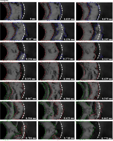
cloud formation and development is shown in Fig. 2. This figure shows representative images selected 198
from case C29 of Table 1; this case corresponds to the erosion tests and sites described previously. 199
The cloud is generated at the outlet of the feed nozzle; this has been a consistent observation for all 200
cases recorded. Then the cavitation cloud grows as it is convected by the flow, until it reaches a 201
maximum distance; this corresponds to the time frame of 0.117ms in Fig. 2. Upstream of this ‘large-202
scale’ cloud structure, which is indicated by the blue dotted line, a second ‘large-scale’ cloud, 203
segmented by the red line is developing, flowing downstream in a similar manner. A cavitation-free 204
zone is visible between them. The follow-up cloud is indicated by the green line and the process 205
repeats itself in a clear vortex shedding mechanism. The estimated shedding frequency is of the order 206
of 1 to 2 kHz for this particular test case; more details about the cloud collapse frequencies are 207
assessed later on. 208
209
Having described the dominant flow structures, image post processing has been employed in an effort 210
to provide estimates of parameters relevant to the spatial and temporal development of the cavitation 211
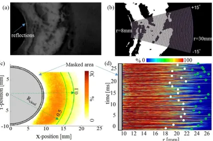
clouds. To do that, the single-colour (grey-scale) images of cavitation recorded (a representative 212
image is shown in Fig. 3a)are turned to binary ones; an example is shown in Fig. 3b. This has been 213
achieved by utilizing the Otsu's method [29]; the threshold value chosen aims to minimize the 214
interclass variance of the black and white pixels. Two averaging procedures have been performed: (a) 215
per pixel and (b) along the circumferential direction, as indicated in Fig. 3b. The field of view 216
analysed is an annular sector with radii 8 mm<r<30 mm and angle θ of 30 degrees. This zone has 217
been divided into 260 concentric arcs. 218
219
At the outlet of the feed nozzle, light reflection on the radius of curvature may not be distinguished 220
from the automatic process converting the raw images to binary ones. For this reason, this area has 221
been masked up to a radial distance of 9.5mm and the corresponding pixels found in this angular zone 222
have not been considered in the post-processing. For the point (pixel) averaging, the temporal mean 223
cavitation presence and its standard deviation have been estimated and contour plots similar to Fig. 3c 224
will be presented in the following section. The mean value can be interpreted as the % number of 225
frames when cavitation is present in a particular location while the corresponding values of standard 226
deviation indicate locations where unsteady cavitation develops. 227
228
Obviously, an error is introduced by the threshold value when performing this process. As possible 229
6
estimated and its spatial distribution is shown by the contour plot of Fig. 3c for case C27; this case has 231
been selected as it exhibits less cavitation, and it has been found to have the maximum error among all 232
cases investigated. It can be seen that the error can take value of up to 20% relative to the mean value 233
of this particular case. The peak values exist in the central part of the cloud development as in these 234
areas it is less accurate to draw clear boundaries between the cavitating and the non-cavitating areas. 235
This error decreases with increasing radial distance and becomes smaller than 5% in the area of cloud 236
collapse. 237
238 239
Fig. 2: Sequence of representative images captured using a frame rate of 77k frames per second
240
[image:7.595.76.520.154.709.2]7
distance of 25mm from the axis of symmetry, which corresponds to the mean distance where erosion 242
sites 2 and 3 have been observed. The coloured dashed lines follow the edge of successive cavitation 243
clouds. 244
245
246
Fig. 3: (a) Representative raw image, (b) binary image after applying a threshold method; the
247
circumferential sectors utilised for post-processing are superimposed. (c) Representative spatial 248
distribution of relative error of the mean cavitation presence in every pixel visualised for case C29; 249
the green lines indicate the cloud length by utilising two different threshold values of 0.5 and 0.1 for 250
its estimation. (d) Representative plot of temporal evolution of the % circumferential area occupied by 251
cavitation as function of distance from the axis of symmetry; the superimposed green circles indicate 252
the locations of maximum cloud extend at the start of collapse and the white circles indicate the cloud 253
length at the end of collapse. 254
255
The second image post-processing method employed estimation of averages along the circumferential 256
direction. This time, the mean of the binary values along each arc has been obtained for every time 257
instant recorded; this can be simply expressed asN1/ (N0+N1), where N0 is the number of pixels
258
exhibiting zero value (no cavitation presence) and N1 is the number of pixels with value equal to one
259
along the selected areas. This ratio represents the percentage area of this circumferential sector 260
occupied by cavitation at a given time step. A representative result from this process is shown in Fig. 261
3d.A few sample points (for clarity of the plot), indicated by the white and green circles, have been 262
superimposed. These circles correspond to radial distances where the mean of the binary values across 263
a circumferential sector has a value of 0.5, indicating that half of this sector is occupied by cavitation 264
at a given time step. This parameter can be utilised to estimate the cloud length at the beginning and 265
ending of the collapse phase. The white circles correspond to time instances at the end of the collapse 266
phase while the green circles at the start of the collapse when the cloud has its maximum extent. By 267
averaging the radial locations corresponding to these two time events, one can obtain the mean of the 268
maximum and minimum cloud extend over all collapse cycles recorded. This is defined here as ‘cloud 269
length’, and represented with Rcloud, and its variation for all cases is presented later on. The maximum
270
value of Rcloud is also indicated on Fig. 3c by the green lines superimposed on this plot for this
271
particular case C27. The one to the left has been estimated by using a value of 0.5. Obviously, other 272
[image:8.595.89.506.121.397.2]8
small clouds isolated from the main cavitation area, and which may not be representative of the mean 274
value across the whole circumferential area. As it is impossible to have an ‘accurate’ estimate, a 275
relative error has been estimated by using a value of 0.1 (implying that only 10% of the 276
circumferential sector is occupied by cavitation at a given time). The value calculated from this 277
assumption is also indicated on Fig. 3c. It can be seen that the cloud length in this case is 278
approximately 2.5mm further downstream relative to the value estimated when 0.5 was used. This 279
gives a relative error of approximately 15% for this particular case. It decreases in cases with more 280
cavitation to levels of around 1-1.5mm which corresponds to about 7% of the cloud length. Finally, 281
fast Fourier transformation (FFT) applied to the temporal evolution of this cloud length can reveal the 282
‘large-scale’ cloud collapse frequency. 283
284
4. CFD Simulations
285
In the absence of quantitative velocity measurements in this configuration, CFD simulations have 286
been performed to provide more insight to the flow structure. The described case was simulated using 287
the in-house CFD solver, GFS. The solver is based on the finite volume methodology. The liquid 288
phase is considered as an incompressible liquid and is resolved in an Eulerian reference frame, 289
whereas cavitation is treated as a discrete phase tracked in Lagrangian frame of reference [30].The 290
bubble motion is governed by the forces due to bubble/liquid interaction, whereas appropriate source 291
terms are added in the continuous phase conservation equations to take into account the effect of the 292
bubble presence inside the liquid flow. The bubble size is governed by the Rayleigh-Plesset equation 293
[30]. The bubble number density for the cavitation inception was set to 1013bubbles/m3, with a size 294
ranging from to 0.5µm to 2µm, following a logarithmic distribution; the aforementioned values are 295
based on literature references [30, 31] and are considered representative of feed water. Since 296
simulating explicitly all bubbles inside the volume would require enormous computational resources, 297
parcels of bubbles are simulated; all bubbles within a parcel are assumed to behave in exactly the 298
same way, thus they have the same velocity field and bubble radius and parcels are introduced in 299
regions where the local pressure is below the saturation (the interested reader is addressed to [30]). In 300
the present simulations the maximum number of bubble parcels was ~45000. The solver is capable of 301
predicting the flow pattern of the fluid/vapour mixture, but, even if the bubbles may expand or 302
collapse, cannot handle compressibility effects and pressure wave propagation in the bubbly medium. 303
304
305
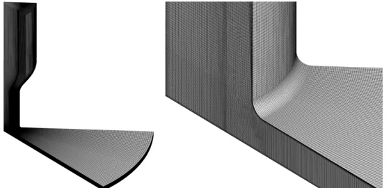
Fig. 4: Computational grid utilized for the CFD analysis; the grid consists of 1.4million cells and has
306
a higher density at the cavitating region 307
308
The simulation performed with GFS was done with a hybrid RANS/LES model [32-34], since it was 309
found that standard traditional URANS models fail to predict the vortex shedding mechanism, while 310
also underestimate the size and the extents of the cavity; this is supported also from other CFD studies 311
in the literature [27, 28]. Moreover, computational predictions with the RANS/LES model suggest the 312
existence of a secondary nucleation site downstream the turn; such fine features are not captured by 313
standard RANS models, as e.g. the k-epsilon model (see Fig. 5 -the comparison is made after 314
obtaining a steady state solution using the k-epsilon model, whereas an average solution has been 315
[image:9.595.163.444.463.598.2]the prediction of a secondary nucleation site cannot be 317
the complexity of the flow field, the prediction of this site 318
underlying mechanisms of cavitation development and suggests further examination in future 319
experiments. The predicted location of the second inception site is within the erosion free zone, lying 320
between 11.3 and 17.2mm (see also 321
between the CFD and the experimental results. 322
the secondary cavitation inception region, downstream the turn, is a stationary vortex core; it appears 323
in such a way, due to the time averaging process for many time instances. In practice, 324
inception site is a highly dynamic and transient feature, generated by the high vorticity downstream 325
the turn, spanning from a radius of 326
αλλαγής. and Fig. 10. This area has the form of 327
~1.5mm.In order to simplify the simulation and decrease the computational cost, due to spatial and 328
temporal resolution requirements of the turbulence model used, only 1/8th of the complete geometry 329
was simulated (see Fig. 1). The computational mesh used consists of approximately 1.4million purely 330
hexahedral cells, refined near the walls and the inlet sharp turn at the feed nozzle exit as showed in 331
Fig. 4. The minimum cell size in the near wall vicinity is 2 332
distance (y+) in the area of interest is ~10 333
kinetic energy spectrum obeys the Kolmogorov 334
at least 10 times less than the sampling frequency; thus both the 335
were considered adequate for the simulations. The simulated condition was for 336
Pdown=19bar (pressure difference 21bar) 337
number of 0.92 (case C29 of Table 1) 338
339
is ~0.13 for the cavitating case. Simulating the same case 340
significantly lower pressure difference 341
38%). 342
343
344
Fig. 5: Comparison of the pressure field from the RANS and the hybrid RANS/LES (averaged in
345
time). The blue iso-surface denotes the region where pressure drops below saturation pressure. 346
simulation conditions correspond to C29, with 347
348
In Fig. 6 the velocity field at a slice of the computational domain is show 349
highly unsteady, with vortices formed downstream the sharp turn 350
the boundary of the separated region 351
leading to the formation of vapour cavities, which travel downstream forming the cavitation clouds 352
a similar pattern as shown from experimental results. 353
9
the prediction of a secondary nucleation site cannot be verified by experimental observations, due to the complexity of the flow field, the prediction of this site may contribute to the
underlying mechanisms of cavitation development and suggests further examination in future location of the second inception site is within the erosion free zone, lying between 11.3 and 17.2mm (see also Fig. 1), could be considered as a rough indication of agreement between the CFD and the experimental results. It must be highlighted here that it is not implied that the secondary cavitation inception region, downstream the turn, is a stationary vortex core; it appears
uch a way, due to the time averaging process for many time instances. In practice,
inception site is a highly dynamic and transient feature, generated by the high vorticity downstream the turn, spanning from a radius of 9 to 20 mm, see also Σφάλµα! Άγνωστη
This area has the form of a Rankine vortex, with a characteristic size of In order to simplify the simulation and decrease the computational cost, due to spatial and temporal resolution requirements of the turbulence model used, only 1/8th of the complete geometry ). The computational mesh used consists of approximately 1.4million purely hexahedral cells, refined near the walls and the inlet sharp turn at the feed nozzle exit as showed in
. The minimum cell size in the near wall vicinity is 2µm and the maximum
) in the area of interest is ~10. From the results obtained, it was tested that the turbulent kinetic energy spectrum obeys the Kolmogorov -5/3 law [35] and the highest temporal frequency was at least 10 times less than the sampling frequency; thus both the temporal and spatial discretizations were considered adequate for the simulations. The simulated condition was for
(pressure difference 21bar), corresponding to a flowrate of 8.16 l/s and a cavitation Table 1). The discharge coefficient Cd, defined as:
(
)
− − = 2 2 . / 1 1 2 in out out in Exp CFD d S S P P Q Cρ
is ~0.13 for the cavitating case. Simulating the same case and ignoring cavitation effects results to a significantly lower pressure difference prediction of ~13bar (Cd~0.16) instead of 21bar (reduction of
Comparison of the pressure field from the RANS and the hybrid RANS/LES (averaged in surface denotes the region where pressure drops below saturation pressure. simulation conditions correspond to C29, with σ~0.9 and Pdown=19bar.
the velocity field at a slice of the computational domain is shown. The velocity field is highly unsteady, with vortices formed downstream the sharp turn, in the shear layer that develops at the boundary of the separated region. Pressure at the vortex cores drops below the saturation pressure,
f vapour cavities, which travel downstream forming the cavitation clouds shown from experimental results.
verified by experimental observations, due to contribute to the understanding of the underlying mechanisms of cavitation development and suggests further examination in future location of the second inception site is within the erosion free zone, lying considered as a rough indication of agreement that it is not implied that the secondary cavitation inception region, downstream the turn, is a stationary vortex core; it appears uch a way, due to the time averaging process for many time instances. In practice, the secondary inception site is a highly dynamic and transient feature, generated by the high vorticity downstream
Σφάλµα Άγνωστη παράµετρος
a Rankine vortex, with a characteristic size of In order to simplify the simulation and decrease the computational cost, due to spatial and temporal resolution requirements of the turbulence model used, only 1/8th of the complete geometry ). The computational mesh used consists of approximately 1.4million purely hexahedral cells, refined near the walls and the inlet sharp turn at the feed nozzle exit as showed in maximum dimensionless wall ained, it was tested that the turbulent and the highest temporal frequency was temporal and spatial discretizations were considered adequate for the simulations. The simulated condition was for Pup=40bar and , corresponding to a flowrate of 8.16 l/s and a cavitation
ignoring cavitation effects results to a instead of 21bar (reduction of
Comparison of the pressure field from the RANS and the hybrid RANS/LES (averaged in surface denotes the region where pressure drops below saturation pressure. The
354 355
356
Fig. 6: Velocity distribution at three
357
the simulated geometry. The simulation conditions correspond to C29, with 358
359 360
In Fig. 7 the instantaneous pressure distribution in the gap between the two disks is shown. 361
of travelling vortices can be found 362
the turn (primary inception point) and at the vortices formed due to the shear layer instability, 363
downstream the turn. Collectively, these vortices act as the secondary nucleation site mentioned 364
above. In both nucleation sites, bubble parcels are intro 365
presence in the flow field. 366
367
368
Fig. 7: Instantaneous pressure distribution at three instances with a time interval of
369
middle slice of the simulated geometry. The continuous line denotes the region where local pressure is 370
below the saturation pressure and the dashed line the radius of 25mm. 371
372
373
Fig. 8: (a) Instantaneous and (b)
374
the inception sites, with local pressure lower than the saturation pressure 375
indicates the radius of 25mm. Note that, due to interpolation during the slice extraction, smoothing 376
inevitably introduced to the vorticity field. 377
10
Velocity distribution at three instances with a time interval of 60µs, taken The simulation conditions correspond to C29, with σ~0.9 and
the instantaneous pressure distribution in the gap between the two disks is shown. found here; as shown, pressure drops below saturation at the vicinity the turn (primary inception point) and at the vortices formed due to the shear layer instability, downstream the turn. Collectively, these vortices act as the secondary nucleation site mentioned above. In both nucleation sites, bubble parcels are introduced, in order to take into account vapour
Instantaneous pressure distribution at three instances with a time interval of
middle slice of the simulated geometry. The continuous line denotes the region where local pressure is pressure and the dashed line the radius of 25mm.
(b) time-averaged vorticity magnitude fields. The continuous line shows , with local pressure lower than the saturation pressure, whereas the dashed line
Note that, due to interpolation during the slice extraction, smoothing introduced to the vorticity field.
taken at the middle slice of ~0.9 and Pdown=19bar.
the instantaneous pressure distribution in the gap between the two disks is shown. Evidence here; as shown, pressure drops below saturation at the vicinity of the turn (primary inception point) and at the vortices formed due to the shear layer instability, downstream the turn. Collectively, these vortices act as the secondary nucleation site mentioned duced, in order to take into account vapour
Instantaneous pressure distribution at three instances with a time interval of 60µs, at the middle slice of the simulated geometry. The continuous line denotes the region where local pressure is
11 378
Furthermore, the CFD results provide an indication of the driving mechanism of the cavity shedding. 379
Indeed, as shown in Fig. 9, the mechanism of the cavity detachment seems to be the re-entrant jet 380
formed between the cavity and the adjacent wall. To be more specific, the cavities formed at the 381
primary inception point at the turn are unstable, thus at some point, a re-entrant jet is formed, starting 382
from the cavity closure location, which forces the cavity to separate from the wall. During the cavity 383
separation, significant vorticity is generated due to the opposing directions of the bulk of the flow and 384
the re-entrant jet. Afterwards, the cavity travels downstream while it may grow further, due to the 385
influence of vorticity. Analysis of the flow field using sampling probe points and performing FFT 386
shows frequencies beginning from 2500Hz till 25000Hz. 387
388
389
Fig. 9. Detailed view during the detachment of a vapour cavity. The effect of the re-entrant jet is
390
visible in the zoomed in region. The contour denotes the vapour fraction and the dashed line denotes 391
the radius of 25mm. 392
393 394
In 395
396
Fig. 10a, the vortical structures formed due to the flow direction change are shown. For the 397
representation, the second invariant of the velocity vector was used [36]. From the results, it is found 398
(a)
that vortex tubes are formed after the sharp turn, organizing in filament 399
structures are found from the experimental 400
vicinity of the nozzle exit), which are convected by the flow and, later on, merge into more 401
complicated structures. Pressure at the vortex cores may drop below the saturation pressure, thus 402
forming moving cavitation inceptions sites. Eventually, vortices are dissipated 403
viscosity, resulting to the collapse of vapour structures. The corresponding plots for the cavitation 404
bubbles utilised and the resulting vapour volume fraction iso 405
406 407
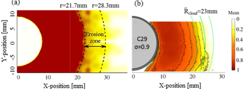
Comparison of those results against the images of the previous 408
409
Fig. 11(σ=0.9and Pdown=19bar) where the 410
both the experiment and the hybrid RANS/LES results, projected on the lower disk; 411
was estimated based on a threshold value which was 5% vapour fraction for the CFD calculations 412
(i.e. if the average vapour fraction at the line 413
is zero).The comparison indicates 414
e.g. the vapour structures begin to collapse at ~20mm from the axis of symmetry (see 415
may disappear just after the 25mm 416
the two disks no experimental data are available 417
the CFD results shows a stronger vapour presence near the upper disk and this could possibly 418
correlate to the extended erosion zone found at the specific disk. 419
420
421
(a)
(b)
12
that vortex tubes are formed after the sharp turn, organizing in filament-like structures (similar structures are found from the experimental results as well, e.g. at Fig. 2 at 0
), which are convected by the flow and, later on, merge into more complicated structures. Pressure at the vortex cores may drop below the saturation pressure, thus forming moving cavitation inceptions sites. Eventually, vortices are dissipated
viscosity, resulting to the collapse of vapour structures. The corresponding plots for the cavitation bubbles utilised and the resulting vapour volume fraction iso-surface of 0.5 is indicated in
Comparison of those results against the images of the previous Fig.
where the time averaged probability of vapour presence both the experiment and the hybrid RANS/LES results, projected on the lower disk;
was estimated based on a threshold value which was 5% vapour fraction for the CFD calculations (i.e. if the average vapour fraction at the line of sight is more than 5%, then the probability is 1, else it indicates similar locations of bubble cloud formation and collapse regions, e.g. the vapour structures begin to collapse at ~20mm from the axis of symmetry (see
may disappear just after the 25mm.Regarding the vapour distribution in the normal direction between the two disks no experimental data are available. However, on average, the vapour distribution from the CFD results shows a stronger vapour presence near the upper disk and this could possibly correlate to the extended erosion zone found at the specific disk.
like structures (similar at 0.506-0.545ms at the ), which are convected by the flow and, later on, merge into more complicated structures. Pressure at the vortex cores may drop below the saturation pressure, thus forming moving cavitation inceptions sites. Eventually, vortices are dissipated due to the fluid viscosity, resulting to the collapse of vapour structures. The corresponding plots for the cavitation
surface of 0.5 is indicated in Fig. 10b.
Fig. 2, is shown in
Fig. 10: (a)Vortical structures, indicated with the second invariant of the velocity gradient tensor and
422
(b) representative bubble parcels 423
corresponds to cavitation volume fraction of 0.5. 424
σ≈0.9 and Pdown=19bar. 425
426
Fig. 11. (a)Time averaged vapour
427
with σ~0.9 and Pdown=19bar. The dashed lines represent the area of 428
specified cavitation number. The region of erosion coincides well with the collapse of the vapour 429
structures. (b) The average experimental 430
431 432
5.Spatial mean cavitation distribution and
433
Having described the flow development we now proceed to the presentation of the results obtained 434
from the post-processing of the collected image 435
shows the spatial distribution of the temporal mean cavitation presence and its standard deviation for 436
selected operating conditions of 437
the middle of the picture. As mentioned earlier, c 438
without any value. This was because in the area of inlet, light 439
of clear images and, thus, the cavitation could not be distinguished automatically. 440
441
A general remark from Fig. 12is that there is a slight asymmetry in the time averaged results. 442
believed to be caused by the asymmetry induced by the outlet pipes. As shown in 443
geometry of the device is not entirely axi 444
pipes that are positioned every 90degress. These pipes probably induc 445
field, imposing a direction of preference, which is manifesting at the lower part of 446
distributions in Fig. 12, for a X-447
the exact effect of the outlet pipes or upstream effects (pipe bends) in the induced asymmetry of the 448
flow field. 449
450
The effect of cavitation number, 451
effect on the extent of cavitation. For high cavitation numbers, mean values have a maximum of less 452
than 50%, which implies that most of the running time no cavitation is present. With decreasing 453
both the appearance becomes more frequent and the cloud propagates further into the flow. For 454
sufficient enough pressure difference, the cloud reaches a ‘steady 455
extend further in the radial direction. The erosion sites 2 and 3, as shown in the previous 456
coincide well with the estimated cloud length, which effectively indicates the area where the 457
cavitation cloud collapses. This zone coincides well with the area of high standard deviation values. 458
Effectively, this area is exposed to successive cloud collapse events. 459
parameters but this time the cavitation number has been kept constant and the back pressure is 460
changing. It is clear that changing t 461
development when σ is kept constant. The cloud length is indicated with the solid green line while the 462
corresponding standard deviation is indicated with the green dotted lines residing to the lef 463
13
(a)Vortical structures, indicated with the second invariant of the velocity gradient tensor and parcels utilized for the simulation of cavitation; the blue iso
corresponds to cavitation volume fraction of 0.5. The simulation conditions correspond to C29, with
vapour probability distribution from the CFD calculations, for case to C29, =19bar. The dashed lines represent the area of erosion of the lower disk
. The region of erosion coincides well with the collapse of the vapour (b) The average experimental vapour probability distribution.
Spatial mean cavitation distribution and cloud length
Having described the flow development we now proceed to the presentation of the results obtained processing of the collected images. The first series of results is presented in
shows the spatial distribution of the temporal mean cavitation presence and its standard deviation for selected operating conditions of Table 1. In each plot, the feed inlet area corresponds to the circle in As mentioned earlier, concentrically with it, a thin zone has been plotted ause in the area of inlet, light reflections have prevented the collection thus, the cavitation could not be distinguished automatically.
is that there is a slight asymmetry in the time averaged results. believed to be caused by the asymmetry induced by the outlet pipes. As shown in
the device is not entirely axisymmetric at the outlet of the disks gap; there are four outlet pipes that are positioned every 90degress. These pipes probably induce a disturbance in the velocity field, imposing a direction of preference, which is manifesting at the lower part of
-position of ~25mm. For the time being, it is not possible to quantify the exact effect of the outlet pipes or upstream effects (pipe bends) in the induced asymmetry of the
The effect of cavitation number, σ, can be realised from Fig. 12b. This parameter has an appreciable effect on the extent of cavitation. For high cavitation numbers, mean values have a maximum of less
%, which implies that most of the running time no cavitation is present. With decreasing both the appearance becomes more frequent and the cloud propagates further into the flow. For sufficient enough pressure difference, the cloud reaches a ‘steady-state’ condition and it does not extend further in the radial direction. The erosion sites 2 and 3, as shown in the previous
he estimated cloud length, which effectively indicates the area where the cavitation cloud collapses. This zone coincides well with the area of high standard deviation values. Effectively, this area is exposed to successive cloud collapse events. Fig. 12
parameters but this time the cavitation number has been kept constant and the back pressure is changing. It is clear that changing the back pressure has only marginal effect of the cavitation is kept constant. The cloud length is indicated with the solid green line while the corresponding standard deviation is indicated with the green dotted lines residing to the lef
(a)Vortical structures, indicated with the second invariant of the velocity gradient tensor and utilized for the simulation of cavitation; the blue iso-surface on conditions correspond to C29, with
from the CFD calculations, for case to C29, erosion of the lower disk for the . The region of erosion coincides well with the collapse of the vapour
Having described the flow development we now proceed to the presentation of the results obtained . The first series of results is presented in Fig. 12. It shows the spatial distribution of the temporal mean cavitation presence and its standard deviation for . In each plot, the feed inlet area corresponds to the circle in oncentrically with it, a thin zone has been plotted reflections have prevented the collection thus, the cavitation could not be distinguished automatically.
is that there is a slight asymmetry in the time averaged results. This is believed to be caused by the asymmetry induced by the outlet pipes. As shown in Fig. 1a, the symmetric at the outlet of the disks gap; there are four outlet e a disturbance in the velocity field, imposing a direction of preference, which is manifesting at the lower part of the spatial For the time being, it is not possible to quantify the exact effect of the outlet pipes or upstream effects (pipe bends) in the induced asymmetry of the
[image:14.595.101.499.129.274.2]of the solid one. The estimated cloud length values are also shown on 464
cavitation number for all back pressure conditions investigated; the standard deviation is also 465
indicated with the vertical bars for all operating points. A clear trend is observed: the cloud length 466
decreases linearly with σ, while there 467
468
469
Fig. 12:Spatial distribution of the mean (time averaged) and
470
the mean) of cavitation presence in the visualised area. The green solid lin 471
mean cloud length and the green dotted lines indicate its standard deviation. 472
pressure for fixed cavitation number (cases 473
back pressure (cases C22, C23, C 474
475
476
Fig. 13: Maximum (dashed lines)
477
cavitation number σ for different downstream pressures; the extent of the erosion zones 2 and 3 478
cavitation number of ~0.9 (see Fig 1) are also superimposed. 479
480
6. Temporal development of cavitation cloud and shedding frequency at location of collapse
481 482
Having described the development of cavitation and its mean distribution, we proceed now to 483
presentation of results revealing more information about its temporal development. In particular, 484
results obtained by utilising the averaging procedures along the circumferential direction, as described 485
earlier, are presented in Fig. 14. The corresponding temporal variation of this mean value is plotted as 486
14
of the solid one. The estimated cloud length values are also shown on Fig. 13
cavitation number for all back pressure conditions investigated; the standard deviation is also indicated with the vertical bars for all operating points. A clear trend is observed: the cloud length
, while there are no significant variations with back pressure.
Spatial distribution of the mean (time averaged) and its standard deviation
of cavitation presence in the visualised area. The green solid line indicates the temporally mean cloud length and the green dotted lines indicate its standard deviation.
pressure for fixed cavitation number (cases C9, C19, C24). (b) Effect of cavitation number for fixed C25of Table 1).
(dashed lines) and minimum (solid lines) cavitation cloud length as function of different downstream pressures; the extent of the erosion zones 2 and 3
(see Fig 1) are also superimposed.
6. Temporal development of cavitation cloud and shedding frequency at location of collapse
Having described the development of cavitation and its mean distribution, we proceed now to sentation of results revealing more information about its temporal development. In particular, results obtained by utilising the averaging procedures along the circumferential direction, as described . The corresponding temporal variation of this mean value is plotted as 13as function of the cavitation number for all back pressure conditions investigated; the standard deviation is also indicated with the vertical bars for all operating points. A clear trend is observed: the cloud length
are no significant variations with back pressure.
standard deviation (expressed as % of e indicates the temporally mean cloud length and the green dotted lines indicate its standard deviation. (a) Effect of back b) Effect of cavitation number for fixed
avitation cloud length as function of different downstream pressures; the extent of the erosion zones 2 and 3 for a
6. Temporal development of cavitation cloud and shedding frequency at location of collapse
15
function of the radial distance from the inlet. The conditions of Fig. 14a correspond to the same 487
cavitation number σ=0.92(cases C9, C19 and C24 of Table 1) while plots of Fig. 14b correspond to 488
conditions where the cavitation number is changing and the back pressure has been kept constant 489
(cases C22, C23 and C25 of Table 1). 490
491
492
Fig. 14: Temporal variation of the circumferentially mean cavitation presence as function of the
493
distance from the axis of symmetry. (a) Effect of back pressure for constant σ (cases C9, C19 and C24 494
of Table 1) and (b) effect of σ for constant back pressure (cases C22, C23 and C25 of Table 1). The 495
vertical dotted while line indicates the mean erosion position of 25mm, visible only in cases where the 496
cavitation number is ~0.9. 497
498
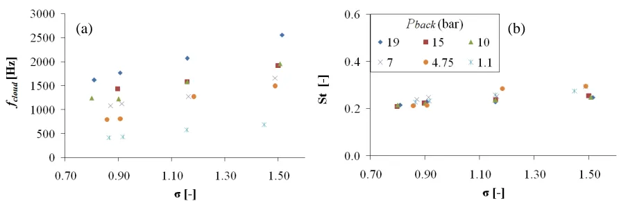
From these plots, it is possible to evaluate the frequency of the cloud appearance/disappearance and 499
collapse. In particular, it is of interest to estimate the main cloud frequency, fcloud, at the distance of 500
25mm which corresponds to the erosion sites 2 and 3 and the corresponding Strouhal number. The 501
fcloud has been evaluated by the fast Fourier transformation (FFT)and it is shown in Fig. 15a for all 502
operating conditions tested. It becomes apparent that CFD predictions of the flow field frequency is 503
higher than that of the experimental shedding frequency. However, direct comparison of the temporal 504
frequencies between the experiment and CFD is not straightforward, since the flow field was not 505
16
obtained from the experiment; experimental frequencies were calculated based on the macroscopic 506
flow features, without taking into account the intricate temporal fluctuations of the flow field. Similar 507
to past observations of cavitation cloud shedding (for example, [18]) the clouds at high σ are small 508
and detach/collapse frequently, whereas at low σ the clouds grow and collapse at a slower rate. The 509
fcloud increases with increasing downstream pressure, due to increase of the flow velocity. This 510
frequency of collapse at the distance of Rcloud as plotted here is similar to the frequency of formation
511
of the ‘large scale’ clouds as estimated earlier from the raw images of Fig. 2. Finally, Fig. 15b shows 512
the Strouhal number, estimates using as length scale the cloud length and the mean velocity of the 513
flow at this location. It is noticeable that the Strouhal number seems to be relatively constant for all 514
tested conditions. 515
516
517
Fig. 15:(a) Cloud collapse frequency (fcloud) at 25mm from the axis of symmetry, as function of σ for 518
different downstream pressures (Pdown). The main frequency has been evaluated utilizing the power
519
spectral density criterion [37]. (b) Strouhal number estimated using the fcloud, the disk distance 520
(2.5mm) and the corresponding mean flow velocity at a radius of 25mm. 521
522 523
7. DISCUSSION OF RESULTS
524 525
Both experimental and computational results show an intricate flow field occurring inside the device; 526
indeed, the flow is highly unsteady showing a periodic behaviour which varies depending on the 527
cavitation number,σ, and Reynolds number, Re. At high cavitation numbers cavitation is not well 528
defined, that is no coherent cavitation structures are formed. As cavitation number decreases, the 529
cavitation influence becomes more significant; cavitation becomes more intense and extends at a 530
larger area, from the nozzle exit to a maximum radial distance of almost 30mm (see Fig. 14). The 531
effect of Reynolds number is primarily linked to the shedding frequency of the cavitation structures; 532
indeed, when considering a constant cavitation number σ, at low back pressures (which also 533
corresponds to low Reynolds number) the shedding frequency is lower. On the other hand, as the 534
downstream pressure is increased, for constant cavitation number σ, the frequency of the shedding 535
also increases. 536
537
When considering a constant downstream pressure, decrease of the cavitation number results to a 538
lengthened and more regular cavity which detaches at lower frequency, while increase of the 539
cavitation number results to smaller and more unstable cavities forming and collapsing at higher 540
frequencies. While this looks counterintuitive, since the decrease of the cavitation number results to 541
increased Reynolds number and, theoretically, to a higher frequency, it is justified by the fact that at 542
low cavitation numbers cavitation structures live longer thus have the time to form agglomerations. In 543
that case, individual vortex cavities are impossible to distinguish, giving the impression of a lower 544
[image:17.595.75.521.233.378.2]17
shedding frequency. Contrary, at higher cavitation numbers at similar Reynolds (thus at higher 545
downstream pressures), cavities tend to remain separate, thus the apparent frequency seems higher. 546
547
The dependence of the Reynolds number on the frequency is justified by the increased vorticity that is 548
being generated downstream the turn. As it was shown from numerical results, the shear layer that 549
forms downstream is unstable and generates significant vorticity. The increase of the Reynolds 550
number with the corresponding increase of the velocity increases the rate of generation of vortices and 551
consequently the frequency of shedding of the resulting cavitating structures. 552
553
A complementary explanation of the unsteadiness of the cavitation shedding process, supported by 554
CFD results, is the influence of the entrant jet, formed at the vicinity of the cavity closure; the re-555
entrant jet has been identified also in the literature as a feature driving the flow unsteadiness for both 556
internal and external flows, e.g. [38, 39]. The distinct phases of the cavity growth and detachment are 557
described below(also shown schematically in Fig. 16); 558
1) Initially cavitation forms at the turn (primary inception site, see also the description in CFD 559
simulations section), due to the rapid acceleration of the liquid. 560
2) The cavity stretches over time due to the local flow conditions, i.e. the shear and the drag, 561
displacing liquid. 562
3) The closure of the cavity is a saddle point [40], thus its location is highly unsteady. A re-entrant jet 563
is formed, which pushes the closure point back towards the turn. The cavity begins to separate from 564
the adjacent wall. 565
4) The re-entrant jet detaches the cavity from the wall, while impinging on the primary inception site. 566
5) The cavity is entirely detached from the primary inception site and the rear part transforms into a 567
bubble cloud. Around the cloud there is significant vorticity, due to the momentum of the re-entrant 568
jet, which is in the opposite direction of the main flow. Moreover, the primary inception site starts to 569
collapse, thus causing erosion at the vicinity of the turn (erosion zone 2). 570
6) The detached cavity transforms into a bubble cloud and moves downstream following the flow. It 571
rapidly rotates due to aforementioned circulation, thus its pressure may fall below saturation and 572
continue to grow, acting as the secondary inception site. The cycle is repeated from (1). 573
18 575
Fig. 16. The cavity shedding cycle: (1) a cavity is formed at the nearby region of the turn, (2) the
576
cavity extends due to shear with the surrounding fluid, (3) the elongation of the cavity stops, while a 577
re-entrant jet is formed, (4) the re-entrant jet detaches the cavity from the adjacent wall, (5) the vapour 578
cavity is entirely detached from the parent cavity at the turn, (6) the detached vapour cavity follows 579
the flow and travels downstream, while it may expand even more due to vorticity. 580
581
The growth and collapse of the vapour clouds is speculated to be linked to the compressibility 582
effects that occur in cavitating flows. Indeed, it is known that the bubbly mixture of 583
vapour/liquid is highly compressible. As mentioned above, a series of vapour cavities is shed 584
from the primary inception site at the turn. These vapour cavities form collectively the bubble 585
cloud, as shown in Fig. 2. As the bubble cloud is travelling downstream, pressure is recovering and 586
vorticity is dissipating due to viscosity. Once the surrounding pressure force counteracts the vorticity 587
induced centrifugal force, the edge of the bubble cloud, approximately at a radial distance of 25mm 588
from the axis of symmetry, starts to collapse. The collapsing bubble cloud may cause a cascade of 589
pressure waves, due to the rapid deceleration of the surrounding water, which could contribute to the 590
erosion in zones 1 and 3. 591
592
8. CONCLUSIONS
593 594
Visualization and CFD results of the cavitation cloud developing inside a hydraulic device have been 595
presented, providing more insight into the details of the sheet/cloud cavitation development for the 596
flow conditions where previous data on material’s response to cavitation erosion have been 597
recorded[1]. As shown from the visualization experiment, the dynamics of the cavitation clouds are 598
complex. In all cases examined, the cloud is generated in the vicinity of the outlet of the feed nozzle. 599
Then the cavitation cloud grows up and is convected by the flow, until it reaches a maximum distance, 600
which varies over time. Afterwards, the cloud collapse is followed by successive formation of clouds. 601
The erosion zones coincide with the areas corresponding to the maximum and minimum cloud length. 602
603
Despite the axisymmetric geometry utilized, instantaneous pictures of cavitation indicate variations in 604
[image:19.595.130.462.70.359.2]