MBotCS: A mobile botnet detection system based on machine learning

City, University of London Institutional Repository

Citation

:

Meng, X. & Spanoudakis, G. (2016). MBotCS: A mobile botnet detection system

based on machine learning. Lecture Notes in Computer Science, 9572, pp. 274-291. doi:

10.1007/978-3-319-31811-0_17

This is the accepted version of the paper.

This version of the publication may differ from the final published

version.

Permanent repository link:

http://openaccess.city.ac.uk/15281/

Link to published version

:

http://dx.doi.org/10.1007/978-3-319-31811-0_17

Copyright and reuse:

City Research Online aims to make research

outputs of City, University of London available to a wider audience.

Copyright and Moral Rights remain with the author(s) and/or copyright

holders. URLs from City Research Online may be freely distributed and

linked to.

City Research Online:

http://openaccess.city.ac.uk/

[email protected]

adfa, p. 1, 2011.

© Springer-Verlag Berlin Heidelberg 2011

machine learning

Xin Meng, George Spanoudakis

City University London, Department of Computer Science, London, UK

{xin.meng.1, g.e.spanoudakis}@city.ac.uk

Abstract. As the use of mobile devices spreads dramatically, hackers have started making use of mobile botnets to steal user information or perform other malicious attacks. To address this problem, in this paper we propose a mobile botnet detection system, called MBotCS. MBotCS can detect mobile device traffic indicative of the presence of a mobile botnet based on prior training us-ing machine learnus-ing techniques. Our approach has been evaluated usus-ing real mobile device traffic captured from Android mobile devices, running normal apps and mobile botnets. In the evaluation, we investigated the use of 5 ma-chine learning classifier algorithms and a group of mama-chine learning box algo-rithms with different validation schemes. We have also evaluated the effect of our approach with respect to its effect on the overall performance and battery consumption of mobile devices.

Keywords: Android, Mobile Botnet, Security, Machine Learning

1

Introduction

nearly 62% of them were part of mobile botnets. The first mobile botnet was an iPh-one botnet, known as iKee.B [17], which was traced back in 2009. iKee.B was not a particularly harmful botnet because iOS is a closed system. Unlike it, Android, which is an open system, has become a major target for mobile botnet creators. Geinimi was the first Android botnet that was discovered in 2010 [37]. Other Android botnets in-clude Android.Troj.mdk, i.e., a Trojan found in more than 7,000 apps that has infected more than a 1m mobile users in China, and NotCompatible.C, i.e., a Trojan targeting protected enterprise networks [27]. Research on mobile botnets (see [16] for related surveys) has looked at device specific botnet detection [22] as well as mobile botnet implementation principles and architectures for creating mobile botnets [11, 34].

In this paper, we describe a proactive approach for detecting unknown mobile bot-nets that we have implemented for Android devices. Our approach is based on the analysis of traffic data of Android mobile devices using machine learning (ML) tech-niques and can be realised through an architecture involving traffic monitors and con-trollers installed on them. The use of ML for detecting mobile botnets has, to the best of our knowledge, also been explored in [12]. However, this study has had some methodological ambiguities. These were related to the exact data set used and, most importantly, to whether the trained ML algorithms were tested against traffic generat-ed by previously unseen botnets or upon a traffic set involving new traffic from bot-nets that were also used to generate traffic in the training set. Furthermore, to the best of our knowledge, so far there has been no implementation of ML detectors running on the mobile device itself neither any evaluation of the impact that this would have on the mobile device (the study in [12] focused on evaluating the performance of the detector learning process).

The experimental study that we report in this paper has been aimed to overcome the above limitations and investigate a number of additional factors, notably: (a) the merit of aggregate ML classifiers, (b) the sensitivity of the detection capability of ML detectors on different types of botnet families, and (c) the actual cost of using ML detectors on mobile devices in terms of execution efficiency and battery consumption. Furthermore, our study has been based on a mobile botnet detection system that we implemented and deployed on a mobile device.

The rest of this paper is organised as follows. Section 2 reviews related work. Sec-tion 3 describes the architecture of MBotCS. SecSec-tion 4 presents the design of our experiments and Section 5 gives an analysis of the results obtained from them. Final-ly, Section 6 outlines conclusions and plans for future work.

2

Related Work

2.1 Special mobile botnet detection techniques

Mobile botnet detection has been studied by Vural et al. [31, 32]. In [31], the authors propose a detection technique based on network forensics and give a list of fuzzy metrics for building SMS (short message service) behavior profiles to use in detec-tion. This approach was improved by introducing detection based on artificial im-mune system principles in [32]. Another system, which can perform dynamic behav-ioral analysis of Android malware automatically, is Copper-Droid [18].

Seo et al. [22] have developed a static analysis tool, called DroidAnalyser, to iden-tify potential vulnerabilities of Android apps and root exploits. This tool processes mobile behaviour in two stages: (a) it checks them against suspicious signatures and (b) it searches app code using pre-fixed keywords. Using (a) and (b), DroidAnalyser can provide warnings before installing an application on a mobile device. However, it cannot detect malware infection from runtime behaviour. Other detection systems, which are based static analysis, include SandDroid [30] and MobileSandbox [26].

2.2 General mobile malware detection techniques

Some of the methods generated for the detection of general mobile malware, can also detect some of the mobile botnets. A monitor of Symbian OS and Windows Mobile smartphone that extracts features for anomaly detection has, for example, been used to monitor logs and detect normal and infected traffic in [21]. However, this system does not run on a mobile device itself.

The approach in [2] includes a static analysis system for analysing Android market applications and uses automated reverse engineering and refactoring of binary appli-cation packages to mitigate security and privacy threats driven by security preferences of the user. The approach is based on a probabilistic diffusion scheme using device usage patterns [1]. The Android Application Sandbox [4] has also been used for both static and dynamic analysis on Android programs and for detecting suspicious appli-cations automatically based on the collaborative detection [20]. This assumes that if the neighbours of a device are infected, the device itself is likely to be infected.

Zhou et al. [35] have developed an approach for detecting “piggybacked” Android applications (i.e., applications that contain destructive payloads or malware code) using: (a) a module decoupling technique that partitions the source code of an applica-tion into primary and non-primary modules and (b) a feature fingerprint technique that extracts various semantic features (from primary modules) and converts them into feature vectors. They have collected more than 1,200 malware samples of Android malware families and characterised them systematically using these techniques.

3

MBotCS system

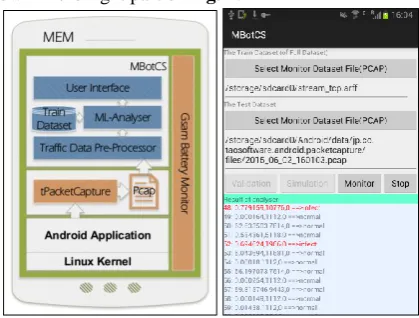
MBotCS is based on the architecture shown in the left part of Fig. 1. As shown in the figure, MBotCS has 4 main components: the traffic data pre-processor, machine learning analyser (ML analyser), user interface and the training dataset. It also uses tPacketCapture [29] and Gsam Battery Monitor [28] to capture mobile traffic and monitor the mobile battery consumption, respectively. All the traffic passing through the mobile device is captured by tPacketCapture and stored in the pcap file on the SDcard of mobile device. The traffic data pre-processor reads the pcap file periodi-cally and converts any incremental data in it into the standard structure file for the ML analyser. The ML analyser trains the classifiers by the training dataset and classifies the captured traffic in real-time as infected or normal. Traffic classifications are shown on the user interface, warning the users to block suspicious applications (i.e., applications that generated traffic classified as infected). The ML analyser is re-trained dynamically when new traffic exceeds a given threshold. Users get warnings through a GUI shown in the right part of Fig. 1.

Fig. 1. The overall architecture and the GUI of MBotCS

4

Methodological setup of the experiments

The implementation of MBotCS has been used in an initial set of experiments that were carried out to evaluate: (1) the accuracy of the classifications produced by it, and (2) its performance in terms of energy consumption and execution time on Android devices. In this section, we describe the methodological set up of these experiments, whilst their results are presented in Section 5.

4.1 Traffic Capture

The mobile device used in the experiments was a Samsung Note 1st _generation (GT-I9228) running Android version 4.1.2 (i.e., Jelly Bean). Jelly Bean is the most fre-quently used version of Android with more 50% of installations in November 2014 [14]. To avoid interference of other applications, the mobile device used for the ex-periment was reset to the default Android OS settings before the exex-periments started.

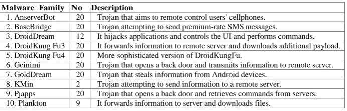
Table 1. Botnet Malware Families

Malware Family No Description

1. AnserverBot 20 Trojan that aims to remote control users' cellphones. 2. BaseBridge 20 Trojan attempting to send premium-rate SMSmessages.

3. DroidDream 12 It hijacks applications and controls the UI and performs commands. 4. DroidKung Fu3 20 It forwards information to remote server and downloads additional payload. 5. DroidKung Fu4 20 More sophisticated version of DroidKungFu.

6. Geinimi 20 Trojan that opens a back door and transmits information to remote server. 7. GoldDream 20 Trojan that steals information from Android devices.

8. KMin 2 Trojan attempting to send information to a remote server.

9. Pjapps 20 Trojan that opens a back door and retrieves commands from servers. 10. Plankton 9 It forwards information to server and downloads files.

To collect traffic data, we deployed 12 normal applications and 163 mobile botnet malware applications, grouped into 10 different families. The normal applications that we used were: Chrome, Gmail, Maps, Facebook, Twitter, Feedly, YouTube, Messen-ger, Skype, PlayNewsstand, Flipboard, and MailDroid. These applications were se-lected due to their popularity. Also to be certain about their genuineness, all of them were downloaded from the Android Official APP Store (Google Play). The botnet malware applications were selected from the MalGenome project [36], according to their level of pandemic risk. MalGenome has collected more than 1200 Android mal-ware applications. The vast majority of these applications (> 90%) are botnets. The botnet malware families that we used are shown in Table 1.

4.2 Dataset Generation

processed to extract features that we considered important for the classifier analysis phase, namely the Source IP Address, Destination IP Address, Protocol, Frame Dura-tion, UDP Packet Size, TCP Packet Size, Stream Index1_{[7] and the HTTP Request} URL. To extract these features we used TShark [33].

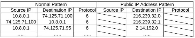
Table 2. Pattern-matching library

Normal Pattern Public IP Address Pattern Source IP Destination IP Protocol Source IP Destination IP Protocol

10.8.0.1 74.125.71.100 6 216.239.32.0 

74.125.71.100 10.8.0.1 6 216.239.32.1

10.8.0.1 74.125.71.95 6 2.14.192.0 

….. ….. ….. …..

The packet traffic data that were obtained from this step were further processed in order to label them as “normal” or “infected”. This step was performed by a script that we developed to compare the mixed traffic file generated by set up B with normal traffic file generated by set up A. More specifically, to label the different packets in the traffic of set up A and set up B, we considered three features of the packets: the Source IP Address, the Destination IP Address andthe used Protocol. The set of le-gitimate (i.e., non-infected) combinations of values of these features was established by analysing the normal traffic data generated from set up A first. These combinations were subsequently expanded further through combinations with legitimate public IP addresses taken from Google Public IP address [13]. Based on this, we generated a three feature pattern-matching library, an extract of which is shown in Table 2. Sub-sequently, every packet in the mixed traffic generated by set up B was compared with the patterns in the library. If the packet had a combination of values for Source IP Address, Destination IP Address, and Protocol matching a pattern in the library, it was labeled as “normal”. Otherwise, it was labeled as “infected”.

Subsequently, we combined the packets with the labels and exported them in csv format (a universal dataset format). Furthermore, as TCP traffic is a stream-oriented protocol (i.e., TCP packets are part of instances of integrated communication between a client and a server, known as streams), we also grouped the individual packets into streams, following TCP. This process yielded two separate data sets: (a) the packet dataset and (b) the stream dataset. The grouping of packets into streams was based on a flag in TCP packets called Stream Index, which indicates the communication stream that each packet belongs to. Thus, an element in the stream dataset was formed by assembling all the packets, which had the same stream index. Streams were labeled as “infected” if they had at least one packet within them that had been labeled as “infect-ed”, and “normal” otherwise.

A preliminary analysis of the datasets generated by the two set ups indicated that all domain name system (DNS) packets, which used the user datagram protocol (UDP) had been labeled as normal. Hence, UDP traffic was excluded from further analysis and the training phase focused on TCP traffic only. This was plausible as botnets involve a series of communications between the bot master and the mobile

botnets that is based on TCP traffic [6]. Following the packets and stream labeling, the features used for training were: Packets/Stream Frame Duration, Packets/Stream Packet Size, and Arguments Number in HTTP Request URL. Overall, the traffic cap-ture and labeling process produced two datasets for the 3rd _{phase of our experiments} (i.e., the classifier analysis phase): (1) the TCP packets dataset, which included 13652 infected packets and 20715 normal packets; and (2) TCP stream dataset, which in-cluded 1043 infected streams and 563 normal streams.

4.3 Classifier Analysis

To analyse the traffic data in the third phase of our experiments, we used 5 supervised machine learning algorithms and a group of machine learning box algorithms. The implementations of these algorithms that use were the ones of WEKA [15], i.e., the open source machine learning analysis toolkit. The algorithms that we used were:

 Naïve Bayes: Naïve Bayes is a family of probabilistic classifiers based on applying Bayes’ theorem. This family assumes that the features of the data items to be clas-sified are strongly independent [19].

 Decision Tree (J48): J48 is a Java implementation of C4.5, i.e., a decision tree based classifier [3].

 K-nearest neighbour (KNN): The k-nearest neighbour (KNN) is a non-parametric classifier algorithm. In KNN, an object is assigned to the class that is the most fre-quent amongst its k nearest neighbours [10].

 Neural Network (MNN): Neural network classification algorithms are used in classification problems characterised by a large number of inputs parameters with unknown relationships [5]. Although in our datasets we had a rather small number of packet/stream features, neural networks were used in the interest of complete-ness. The specific algorithm that we used was the multi-layer perceptron.

 Support Vector Machine (SMO): Support Vector Machine is a supervised associ-ated learning algorithm, using Platt’s sequential minimal optimization (SMO). In addition to single algorithms, we used ML boxing, a technique where classifica-tions of the individual ML algorithms are aggregated in order to improve the accuracy of results. More specifically, we used three aggregation methods:

 ML-BOX (AND): In this aggregate classifier, an instance of the dataset was classi-fied as infected if ALL the individual classifiers indicated it as infected. Other-wise, the instance was classified as normal.

 ML-BOX (OR): In this aggregate classifier, an instance of the dataset was classi-fied as infected if AT LEAST ONE the individual classifiers indicated it as infect-ed. Otherwise, the instance was classified as normal.

 ML-BOX (HALF): In this aggregate classifier, an instance of the dataset was clas-sified as infected if MORE THAN HALF of the individual classifiers indicated it as infected. Otherwise, the instance was classified as normal.

ML-BOX+(HALF), if the J48 and KNN algorithms classified the instance of dataset in the same class, ML-BOX+(HALF) generated the same common classification. When J48 and KNN were in disagreement, ML-BOX+ (HALF) generated a classification based on the outcome of the 3 remaining classifiers only.

To validate the experimental training results, we used 3 validation schemes based on K-fold cross validation and 10% split validation.

K-fold cross validation is a common technique for estimating the performance of a ML classifier. According to it, in a learning training involving m training examples, the examples are initially arranged in random orders and then they are divided into k folds. A classifier is then trained with examples in all folds but fold i (i = 1 . . . k), and its outcomes are tested using the examples in fold i. Following this training-testing process, the classification error of a classifier is computed by E = (

i=1..Kni)/m where 𝑛𝑖 is the number of the wrongly classified examples in fold 𝑖 and 𝑚 is the number of

training examples. Based on this scheme, we used 90-10% 10-fold and 50-50% 2-fold cross validation, which are two typical validation approaches in ML. Split validation is simpler as it divides the training dataset into two parts, one part containing data used only for training and another part containing data used only for testing. In 90-10% split validation, 90% of the data are selected as training dataset and 90-10% as the test dataset.

The analysis of the performance of classifiers was also based on two different for-mulations of the training and test data sets. In the first formulation (experiment 1), both the training and the test data sets could include data from the same malware fam-ily, although the two data sets were disjoint. Hence, in this experiment, classifiers could have been trained with instances of traffic from a malware family that they needed to detect. In the second formulation (experiment 2), the training and test data sets were restricted to include only data from different malware families. Hence, in this experiment, the classifiers were tested on totally unknown malware families (i.e., malware families whose infected data traffic had not been considered at all in the training phase).

5

Experimental Results

5.1 Basic observations

To evaluate and compare the results arising in the different experiments, we used three performance measures: the True Positive Rate (TPR), the False Positive Rate (FPR) and Precision. These measures are used typically for the evaluation of ML based classification and are defined as follows:

True Positive Rate: TPR = TP/ (TP + FN) (aka Recall) (1) False Positive Rate: FPR = FP/ (TN + FP) (2)

Precision = TP/ (TP + FP) (3)

number of normal data that were incorrectly classified as infected by an ML algo-rithm; and False negative (FN) is the number of infected data that were incorrectly classified as normal by an ML algorithm.

Experiment 1. As discussed in Section 4, all the UDP protocol traffic in the dataset was labeled normal and was filtered out in the subsequent analysis. Thus, the attrib-utes that we used in the experiment were frame duration, TCP packet size and the number of arguments in the HTTP requests URL. Also classifications were performed separately for the stream and packet data sets using all basic classifier algorithms. Hence, we carried out 30 groups of basic algorithm experiments (5 classifier algo-rithms × 3 validation schemes × 2 data sets) and 18 groups of ML-BOX experiments (6 box algorithms × 3 validation schemes × 1 data set).

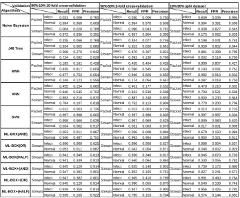
Table 3. Results of experiment 1

The results of the experiments for the atomic and aggregate classifiers from exper-iment 1 are shown in Table 3. The table shows the recall, precision and FPR measures for stream and packet data separately and for different validation set ups (90-10% 10-fold validation, 50-50% 2-fold validation, and 10-90% split validation). The main overall observation from Table 3 was that the results in the case of packet level traffic were not encouraging and that the results for stream traffic were consid-erably better.

90%-10% 10-fold cross-validation 50%-50% 2-fold cross-validation 10%-90% split dataset

Recall FPR Precision Recall FPR Precision Recall FPR Precision

Infect 0.031 0.006 0.760 Infect 0.030 0.006 0.750 Infect 0.609 0.006 0.994 Normal 0.994 0.969 0.609 Normal 0.994 0.970 0.608 Normal 0.994 0.391 0.609 Infect 0.064 0.028 0.788 Infect 0.096 0.043 0.781 Infect 0.938 0.827 0.645 Normal 0.972 0.936 0.391 Normal 0.957 0.904 0.395 Normal 0.173 0.062 0.635 Infect 0.335 0.066 0.769 Infect 0.344 0.077 0.746 Infect 0.198 0.041 0.763 Normal 0.934 0.665 0.680 Normal 0.923 0.656 0.681 Normal 0.959 0.802 0.644 Infect 0.908 0.276 0.842 Infect 0.870 0.307 0.821 Infect 0.881 0.398 0.780 Normal 0.724 0.092 0.829 Normal 0.693 0.130 0.766 Normal 0.602 0.119 0.760 Infect 0.183 0.161 0.428 Infect 0.455 0.404 0.426 Infect 0.909 0.807 0.427 Normal 0.839 0.817 0.609 Normal 0.596 0.545 0.624 Normal 0.193 0.091 0.761 Infect 0.877 0.752 0.654 Infect 0.946 0.826 0.650 Infect 0.982 0.913 0.633 Normal 0.248 0.123 0.556 Normal 0.174 0.054 0.667 Normal 0.087 0.018 0.750 Infect 0.455 0.154 0.660 Infect 0.461 0.177 0.632 Infect 0.479 0.210 0.602 Normal 0.846 0.545 0.702 Normal 0.823 0.539 0.698 Normal 0.790 0.521 0.696 Infect 0.893 0.216 0.870 Infect 0.887 0.248 0.853 Infect 0.800 0.230 0.848 Normal 0.784 0.107 0.818 Normal 0.752 0.113 0.804 Normal 0.770 0.200 0.706 Infect 0.012 0.003 0.726 Infect 0.012 0.003 0.726 Infect 0.013 0.003 0.733 Normal 0.997 0.988 0.605 Normal 0.997 0.988 0.605 Normal 0.997 0.987 0.604 Infect 0.998 0.966 0.626 Infect 0.997 0.969 0.625 Infect 0.999 0.983 0.620 Normal 0.034 0.002 0.917 Normal 0.031 0.003 0.870 Normal 0.017 0.001 0.909 Infect 0.053 0.011 0.887 Infect 0.036 0.008 0.884 Infect 0.679 0.150 0.884 Normal 0.946 0.487 0.751 Normal 0.992 0.964 0.389 Normal 0.850 0.321 0.612 Infect 0.996 0.969 0.625 Infect 0.996 0.958 0.627 Infect 0.998 0.954 0.637 Normal 0.053 0.011 0.887 Normal 0.042 0.004 0.871 Normal 0.046 0.002 0.929 Infect 0.941 0.349 0.813 Infect 0.936 0.340 0.817 Infect 0.945 0.670 0.703 Normal 0.941 0.349 0.813 Normal 0.660 0.064 0.864 Normal 0.330 0.055 0.782 Infect 0.845 0.129 0.914 Infect 0.835 0.148 0.902 Infect 0.759 0.173 0.880 Normal 0.947 0.382 0.801 Normal 0.852 0.165 0.761 Normal 0.827 0.241 0.672 Infect 0.947 0.382 0.801 Infect 0.945 0.410 0.789 Infect 0.891 0.460 0.764 Normal 0.845 0.129 0.914 Normal 0.590 0.055 0.870 Normal 0.540 0.109 0.746 Infect 0.939 0.359 0.814 Infect 0.847 0.205 0.900 Infect 0.856 0.426 0.782 Normal 0.939 0.165 0.922 Normal 0.795 0.153 0.704 Normal 0.574 0.144 0.691

Validation Algorithms

Naive Bayesian

Packet Packet Packet

Stream Stream Stream

J48 Tree

Packet Packet Packet

Stream Stream Stream

MNN

Packet Packet Packet

Stream Stream Stream

KNN

Packet Packet Packet

Stream Stream Stream

SVM

Packet Packet Packet

Stream Stream Stream

This could be explained as follows. In TCP communication, the server and client should make a connection by a 3-way handshake, then send transfer data (payload packets) in fragments to stay below a maximum transmission unit (MTU). Also for each data transfer, the receiver sends an acknowledgement signal packet (ACK sig-nal). Finally, the initiator sends a FIN signal packet to end the communication. In our experiments, data of normal and infected applications were labeled by the source and destination IP address of each traffic instance. In the case of the packet dataset, there was a large number of FIN and ACK packets labeled as “infected” due to the used IP addresses. The remaining features of these packets, however, were similar to FIN and ACK packets labeled as “normal”. Thus, the classifiers could not distinguish between them. In the case of the stream dataset, however, FIN and ACK packets were grouped into single streams and hence their own characteristics did not feature prominently in the training and testing data sets. Hence, the classifiers were not misled by these sig-nal packets in cases where they had the same features as payload packets and, conse-quently, the performance of the stream dataset was better than that of the packet da-taset.

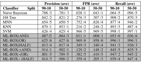
Focusing on stream traffic only, Table 4 shows the average recall, TPR and preci-sion across for the two validation schemes with the best outcome (i.e., the 90-10 and 50-50 k-fold validation) in the case of infected traffic, and the relative ranking of each algorithm given the each of the evaluation measures. In the case of KNN, for exam-ple, the table shows “.870 /1” under precision for the 90-10 validation scheme. This means that the precision of KNN was .870 for the 90-10 scheme and that this algo-rithm was ranked 1st _{amongst the atomic algorithms. The results show a mixed} pic-ture. In particular, KNN and J48 were the best two atomic algorithms in terms of pre-cision; KNN and J48 were the best two atomic algorithms in terms of recall; and Na-ïve Bayesian and KNN were the best two atomic algorithms in terms of FPR. The outcome was the same in the case of precision and FPR for the 50-50% scheme but in this case the ranking of atomic algorithms changed for recall (SVM still turned out as best but was followed by MNN).

Table 4. Ranking of algorithms for infected stream traffic in Experiment 1

Precision (ave) FPR (ave) Recall (ave) Classifier Split 90-10 50-50 90-10 50-50 90-10 50-50

Naïve Bayesian .788 /3 .781/ 3 .028 /1 .043 /1 .064 /5 .096 /5 J48 Tree .842 /2 .821/ 2 .276 /3 .307 /3 .908 /2 .870 /3 MNN .654 /5 .650/ 5 .752 /4 .826 /4 .877 /4 .946 /2 KNN .870 /1 .853 /1 .216 /2 .248 /2 .893 /3 .887 /4 SVM .626 /4 .625/ 4 .966 /5 .969 /5 .998 /1 .997 /1 ML-BOX(AND) .887 /2 .884 /3 .011 /1 .008/ 1 .053 /6 .036 /6 ML-BOX(OR) .625 /6 .627 /6 .969 /6 .958 /6 .996 /1 .996 /1 ML-BOX(HALF) .813 /4 .817 /4 .349 /3 .340 /4 .941 /3 .936/ 3 ML-BOX+(AND) .914 /1 .902 /1 .129 /2 .148 /2 .845 /5 .835/ 5 ML-BOX+(OR) .801 /5 .789 /5 .382 /5 .410 /5 .947/ 2 .945 /2 ML-BOX+ (HALF) .814 /3 .900 /2 .359 /4 .205 /3 .939 /4 .847 /4

algorithms produced the best recall for infected traffic (i.e., about 99% and 95%, re-spectively) for both validation schemes. In terms of precision and FPR, the best two algorithms were ML-BOX+(AND) and ML-BOX(AND), albeit the different order of their ranking under each of these measures. ML-BOX(OR) and ML-BOX+(OR) yielded a higher recall than the individual algorithms because they classified as in-fected the union of the streams classified as such by any of these algorithms (i.e., a superset of all the sets of infected streams returned by the individual algorithms). ML-BOX(AND) and ML-BOX+(AND) yielded a higher precision than individual algo-rithms as they classified as infected the intersection of the streams that were classified as such by these algorithms (i.e., a subset of all the sets of infected streams returned by the individual algorithms).

Comparing the results across different validation schemes, the results in terms of precision and FPR in the case of 90-10% 10-fold validation were better than those of the 50-50% 2-fold validation for most algorithms, although no notable differences amongst these two schemes were observed for recall.

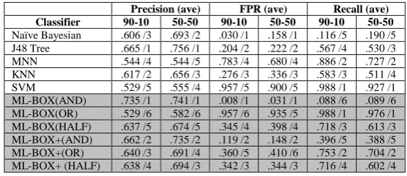
Experiment 2. The second experiment focused on assessing the capability of classifi-ers to detect totally unknown mobile botnet malware. To do so, we partitioned the infected stream dataset into different subsets containing only data from the individual mobile botnet malware families. This produced 9 sets of infected data coming from all families in Table 1 except from family 8 which did not produce any infected data. The 9 sets of infected data were mixed with a random selection of 10% of normal stream data to formulate an infected family data set. Subsequently, we used ~90-10% 10-fold validation by selecting data streams from 8 families and testing it on the re-maining 1 family and ~50-50% 2-fold validation by selecting data streams from 5 families and testing it on the remaining 4 families.

Table 5. Ranking of algorithms for infected stream traffic in Experiment 2

Precision (ave) FPR (ave) Recall (ave) Classifier 90-10 50-50 90-10 50-50 90-10 50-50

Naïve Bayesian .606 /3 .693 /2 .030 /1 .158 /1 .116 /5 .190 /5 J48 Tree .665 /1 .756 /1 .204 /2 .222 /2 .567 /4 .530 /3 MNN .544 /4 .544 /5 .783 /4 .680 /4 .886 /2 .727 /2 KNN .617 /2 .656 /3 .276 /3 .336 /3 .583 /3 .511 /4 SVM .529 /5 .555 /4 .957 /5 .900 /5 .988 /1 .927/1 ML-BOX(AND) .735 /1 .741 /1 .008 /1 .031 /1 .088 /6 .089 /6 ML-BOX(OR) .529 /6 .582 /6 .957 /6 .935 /5 .988 /1 .976 /1 ML-BOX(HALF) .637 /5 .674 /5 .345 /4 .398 /4 .718 /3 .613 /3 ML-BOX+(AND) .662 /2 .735 /2 .119 /2 .148 /2 .396 /5 .388 /5 ML-BOX+(OR) .640 /3 .691 /4 .360 /5 .410 /6 .753 /2 .704 /2 ML-BOX+ (HALF) .638 /4 .694 /3 .342 /3 .344 /3 .716 /4 .602 /4

algorithm was ranked 1st _{amongst the atomic algorithms). Table 6 shows the results} for each of the individual malware families as produced in the 90-10 scheme.

Table 6. Recall/FUR/Precision for individual botnet families (90-10 scheme)

The main observations drawn from experiment 2 are:

(i) The precision, recall and FPR of all classifiers (both the atomic and the agggated ones) dropped w.r.t experiment 1, as it can be seen by contrasting the re-call and precision figures for the 90-10 and 50-50 cross validation column for stream data in Table 3 with the corresponding figures in Table 5. The drop was more significant in the case of recall.

(ii) The cross validation with the 50-50 slit generated better outcomes than the 90-10 Malware Family

Measures Recall FPR Precision Recall FPR Precision Recall FPR Precision Naive Bay esian 0.059 0.03 0.846 0.05 0.03 0.818 0.571 0.03 0.667

J48 Tree 0.636 0.152 0.922 0.403 0.182 0.859 0.714 0.242 0.238 M NN 0.695 0.53 0.788 0.994 0.864 0.759 1 0.864 0.109

KNN 0.642 0.288 0.863 0.768 0.242 0.897 0.857 0.303 0.231

SVM 1 0.955 0.748 1 0.955 0.742 1 0.97 0.099 M L-BOX(AND) 0.032 0 1 0.028 0.015 0.833 0.571 0.015 0.8

M L-BOX(OR) 1 0.955 0.748 1 0.955 0.742 1 0.97 0.099 M L-BOX(HALF) 0.658 0.227 0.891 0.796 0.318 0.873 0.857 0.424 0.176 M L-BOX+(AND) 0.556 0.136 0.92 0.376 0.121 0.895 0.714 0.136 0.357 M L-BOX+(OR) 0.722 0.303 0.871 0.796 0.303 0.878 0.857 0.409 0.182 M L-BOX+(HALF) 0.658 0.227 0.891 0.796 0.303 0.878 0.857 0.409 0.182

Malware Family

Measures Recall FPR Precision Recall FPR Precision Recall FPR Precision Naive Bay esian 0.054 0.03 0.846 0.018 0.03 0.333 0.2 0.03 0.5

J48 Tree 0.639 0.182 0.916 0.145 0.227 0.348 0.6 0.258 0.261 M NN 0.917 0.788 0.783 0.745 0.848 0.423 0.9 0.848 0.138 KNN 0.561 0.227 0.885 0.418 0.212 0.622 0.8 0.303 0.286 SVM 0.995 0.955 0.764 1 0.955 0.466 0.9 0.955 0.125 M L-BOX(AND) 0.01 0 1 0 0.015 0 0.1 0.015 0.5

M L-BOX(OR) 0.995 0.955 0.764 1 0.955 0.466 0.9 0.955 0.125 M L-BOX(HALF) 0.795 0.288 0.896 0.364 0.348 0.465 0.8 0.409 0.229 M L-BOX+(AND) 0.4 0.121 0.911 0.145 0.091 0.571 0.6 0.152 0.375 M L-BOX+(OR) 0.8 0.288 0.896 0.418 0.348 0.5 0.8 0.409 0.229 M L-BOX+(HALF) 0.785 0.288 0.894 0.364 0.348 0.465 0.8 0.409 0.229

Malware Family

Measures Recall FPR Precision Recall FPR Precision Recall FPR Precision Naive Bay esian 0.026 0.03 0.333 0.06 0.03 0.778 0.004 0.03 0.333

J48 Tree 0.763 0.242 0.644 0.607 0.152 0.877 0.593 0.197 0.917

M NN 0.974 0.727 0.435 0.752 0.727 0.647 1 0.848 0.813 KNN 0.447 0.303 0.459 0.667 0.303 0.796 0.086 0.303 0.512 SVM 1 0.955 0.376 1 0.955 0.65 1 0.955 0.794 M L-BOX(AND) 0.026 0 1 0.026 0.015 0.75 0 0 0

M L-BOX(OR) 1 0.955 0.376 1 0.955 0.65 1 0.955 0.794 M L-BOX(HALF) 0.842 0.394 0.552 0.692 0.333 0.786 0.654 0.364 0.869 M L-BOX+(AND) 0.342 0.136 0.591 0.41 0.045 0.941 0.025 0.136 0.4

M L-BOX+(OR) 0.868 0.409 0.55 0.863 0.409 0.789 0.654 0.364 0.869

M L-BOX+(HALF) 0.842 0.394 0.552 0.692 0.333 0.786 0.654 0.364 0.869

3 (7 infect streams)

6 (10 infect streams)

10 (243 infect streams) 1 (187 infect streams) 2 (181 infect streams)

4 (205 infect streams) 5 (55 infect streams)

split in terms of precision, recall and FPR for all algorithms. This was probably due to over fitting, as in the 90-10 scheme we found recall to correlate positively with the training-to-test data set size (TTTS) ratio and precision to correlate with TTTS negatively: the correlation coefficients were 0.41 for TTTS/Recall, and – 0.90 for TTTS/Precision.

(iii) Results were poor for all families with a low number (<50) of infected streams (i.e., families 3, 5, 6, 7). Generally, recall

(iv) The algorithms J48 and Naïve Bayesian have had the best performance in terms of precision and FPR amongst the atomic algorithms in the 90-10 and 50-50 scheme. However, their performance in terms of recall was not so good (0.567 and 0.116, respectively). In terms of recall, the best performers amongst single algorithms were SVM and MNN. However, both these algorithms had low pre-cision and high FRP rates.

(v) ML-BOX (AND) and ML-BOX+(AND) have had the best performance in terms of precision and FPR amongst the aggregate (box) algorithms in the 90-10 and 50-50 schemes. However, their performance in terms of recall was not poor (0.088 and 0.396, respectively). In terms of recall, the best performers amongst box algorithms were BOX(OR) and BOX+(OR). However, only ML-BOX+(OR) appeared to have acceptable precision and FPR rate.

(vi) Recall and FPR were found to correlate positively with the size of the infected data set of a family and precision was found to correlate negatively with it.

5.2 Performance

Although the performance of mobile devices has improved significantly in recent years, their computing and energy capabilities are still limited. Therefore, a system deployed on a mobile device should be designed to minimize the demand of such resources. Hence, in our experiments we should also evaluate the execution time and battery consumption of MBotCS. The mobile device used in this evaluation was a GT-I9228 with 1440 MHz CPU clock, 1 GB of RAM and battery of 2500 mAh. MBotCS, tPacketCapture, and Gsam Battery Monitor had been installed on it. Then we made a random selection of 10 botnet applications and 10 normal applications of those indicated in Sec. 4.1 and run the evaluation experiment for 12 hours. The set up of the experiment involved the following sequence of steps:

(1) Charged fully the battery of the mobile device and installed all the applications. (2) Launched the Gsam Battery Monitor, tPacketCapture and MBotCs applications. (3) Launched the normal and infected applications mentioned above and run 5

minutes for each application to simulate user behaviours, and the remaining ex-periment time keep the mobile device on standby.

(4) Gathered and analysed results.

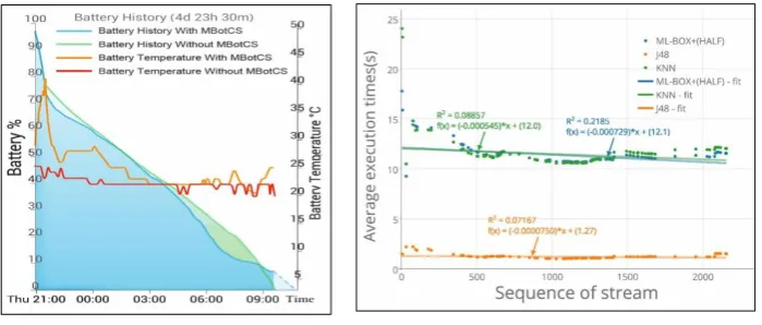
Fig. 2. Battery Consumption Fig. 3. The ML-Analyser Execution Time

Results - Battery Consumption: The graphs of battery consumption in percentage terms and battery temperature during the experiment is shown in Fig. 2. According to the figure, the battery consumption was not affected significantly by the use of MBotCS. In particular, the use of MBotCS consumed 0.5% of the total battery usage of the device during the period of its deployment. Of this, 0.2% was the battery usage caused by tPacketCapture. These figures show that MBotCS has had a very low ener-gy effect on the battery consumption of the device.

Execution Time: When activated,MBotCS checks the pcap file periodically, and if new traffic is captured, it scans and analyses it. In these scans, the scan sequence number (𝑠𝑞) is recorded. Using the J48, KNN and ML-BOX+(HALF) classifiers in the ML-Analyser, we recorded the number of streams (𝑁𝑠𝑞) in the new traffic and the total execution time (𝑇𝑠𝑞) for analysing the new traffic. Fig. 3 shows the average execution times for the three classifiers, computed by the formula 𝑇𝑎𝑣𝑒𝑠𝑞 =

∑𝑠𝑞 𝑇𝑠𝑞

𝑖=0 / ∑𝑠𝑞𝑖=0𝑁𝑠𝑞 (the average for sequence number 100, for instance, is the

aver-age of execution time of a classifier over all stream instances from 1 to 100). The figure also shows the fitted curves for the average execution times of these algo-rithms.

The results show that the average execution time of J48 across all executions was 1.216 seconds with a standard deviation of 0.228 and the average of KNN across all executions was 11.562 seconds with a standard deviation of 1.779. The average of ML-BOX+ (HALF) across all executions was 11.387 seconds with a standard devia-tion of 1.087. A t-test check showed the statistical significance of the observed differ-ences between the average execution times of J48 and KNN at α = 0.05 (p−value = 2.701E−91 << 0.05), confirming that J48 have had better performance than KNN.

5.3 Discussion

Regarding the observed differences across the different classifier algorithms, it should be noted that a relevant factor is the total number of streams in the stream dataset. This number was not very high (even though we captured a large number of individu-al packets). Also a statisticindividu-al anindividu-alysis of the vindividu-alues of the features in the dataset showed that these values did not have a normal distribution. Furthermore, features were not independent (e.g., the TCP size depends on the arguments of an HTTP re-quest). For datasets with such characteristics, certain classifier algorithms such as the Naïve Bayesian classifier are not suitable (as NB requires the features in the dataset to be independent and have normally distributed values). The main threats to the validity of the outcomes of our experiments are summarised below:

(1) All the traffic was captured on only one mobile device, so contingency factors of hardware and software might have not been fully accounted for (e.g., dis-connections from the network, crashes of applications due to insufficient memory).

(2) In general, there is an active period for every malware application. Some bot-nets may change the botmaster server or go through updates of the malicious code in the infected applications. None of these was reflected in the traffic that we considered.

(3) The availability of a bot master could not be guaranteed in our experiments. Therefore, the considered botnets may have further interactions that were not captured in the traffic that we used.

(4) The size of the stream dataset used in the experiments was relatively small and therefore the observed results need to be confirmed by larger experiments.

6

Conclusions and future work

In this paper, we have presented MBotCS, a mobile botnet detection system imple-mented for Android mobile devices that uses machine learning to detect traffic gener-ated by mobile botnet malware.

To evaluate the feasibility of this approach for mobile botnet detection, we carried out a series experiments. These experiments have shown promise in detecting botnets. Detection was more effective in cases where the ML classifiers had been trained using traffic of a given botnet (albeit different from the traffic used in the test) than in cases where ML classifiers had to detect totally unknown botnets. The experiments also showed that detection was more effective for stream traffic than for packet traffic and that aggregate (box) ML algorithms were more effective than atomic algorithms. They also showed significant differences between the execution times of different ML algorithms on the mobile device and low battery consumption, which is a prerequisite for the feasibility of the approach on mobile devices.

want to explore the use of unsupervised classification and contrast its outcomes with supervised classification, and investigate the reasons underpinning the differences in the performance of the basic ML algorithms.

The datasets that we used for the experiments reported in this paper, and the scripts for their generation are available from: http://emx2.co.uk/mbotcs/.

References

1. Alpcan, T., Bauckhage, C., Schmidt, A.D.: A Probabilistic Diffusion Scheme for anomaly Detection on Smartphones. In: Information Security Theory and Practices. Security and Privacy of Pervasive Systems and Smart Devices, pp. 31–46. Springer (2010)

2. Batyuk, L., Herpich, M.: Using static analysis for automatic assessment and mitigation of unwanted and malicious activities within Android applications. 2011 6th Int. Conf. Mali-cious Unwanted Software, pp. 66–72. (2011).

3. Bhargava, D., et al.: Decision Tree analysis on j48 Algorithm for Data Mining. Int. Journal of Advanced Research in Computer Science & Software Engineering, 3(6): 1114–1119 (2013)

4. Bläsing, T., et al.: An android application sandbox system for suspicious software detec-tion. Proceedings of the 5th IEEE International Conference on Malicious and Unwanted Software, pp. 55–62 (2010).

5. Boland, M.V., Murphy, R.F.: A neural network classifier capable of recognizing the pat-terns of all major subcellular structures in fluorescence microscope images of HeLa cells, Bioinformatics, 17(12), 1213-1223 (2001)

6. Braun, L., Münz, G., Carle, G.: Packet sampling for worm and botnet detection in TCP connections. Proceedings of the 2010 IEEE/IFIP Network Operations and Management Symposium, NOMS 2010. pp. 264–271 (2010).

7. Chappell, L.A., Combs, G.: Wireshark 101: Essential Skills for Network Analysis. Proto-col Analysis Institute, Chappell University (2013).

8. Funk C., Garnaeva M.: Kaspersky security bulletin (2013) https://securelist.com/ analy- sis/kaspersky-security-bulletin/58265/kaspersky-security-bulletin-2013-overall-statistics-for-2013

9. Cisco: Cisco visual networking index: Global mobile data traffic forecast update, 2014-2019. Tech. rep. (2015). http://www.cisco.com/en/US/solutions/collateral/ns341/ns525/-ns537/ns705/ns827/white_paper_c11-520862.html

10. Cunningham, P., Delany, S.J.: k-nearest neighbour classifiers. Multiple Classifier Systems pp. 1–17 (2007)

11. Eslahi, M., Salleh, R., Anuar, N.B.: MoBots: A new generation of botnets on mobile de-vices and networks. 2012 Int. Symposium on Computer Applications and Industrial Elec-tronics. 262–266 (2012).

12. Feizollah, A., et al..: A study of machine learning classifiers for anomaly-based mobile botnet detection. Malaysian Journal of Computer Science 26(4), 251–265 (2014)

13. Google: Google IP address ranges (Accessed June 2015), https://support.google.com/a/-answer/60764?hl=en

14. Google: Dashboards (Accessed June 2015), https://developer.android.com/about/-dashboards/index.html

16. Kalige, E., Burkey, D., Director, I. P. S.: A case study of eurograbber: How 36 million eu-ros was stolen via malware. Versafe (White paper) (2012)

17. Porras, P., Saidi, H., Yegneswaran, V.: An analysis of the ikee.b iphone botnet. In: Securi-ty and Privacy in Mobile Information and Communication Systems, pp. 141–152. Springer (2010)

18. Reina, A., Fattori, A., Cavallaro, L.: A system call-centric analysis and stimulation tech-nique to automatically reconstruct android malware behaviors. EuroSec, April (2013) 19. Rish, I.: An empirical study of the naive Bayes classifier. IJCAI 2001 Workshop on

Em-pirical Methods in Artificial Intelligence vol. 3, no. 22, pp. 41-46 (2001)

20. Schmidt, A. D., et al.: Static analysis of executables for collaborative malware detection on android. In: IEEE International Conference on Communications 2009, pp. 1–5. (2009) 21. Schmidt, A. D., et al.: Monitoring smartphones for anomaly detection. Mobile Networks

and Applications 14(1), 92–106 (2009)

22. Seo, S. H., Gupta, A., Sallam, A. M., Bertino, E., Yim, K.: Detecting mobile malware threats to homeland security through static analysis. Journal of Network and Computer Applications 38, 43–53 (2014)

23. Shabtai, A., Kanonov, U., Elovici, Y.: Detection, alert and response to malicious behavior in mobile devices: Knowledge-based approach. In: Kirda, E., et al. (eds.) Recent Advances in Intrusion Detection, Lecture Notes in Computer Science, vol. 5758, pp. 357–358. (2009) 24. Shabtai, A., el. Al.: "Andromaly": a behavioral malware detection framework for android

devices. Journal of Intelligent Information Systems 38(1), 161–190 (2012)

25. Shahar, Y.: A framework for knowledge-based temporal abstraction. Artificial Intelligence 90(1): 79–133 (1997)

26. Spreitzenbarth, M., et al.: Mobile-sandbox: Having a deeper look into android applica-tions. 28th _{Annual ACM Symposium on Applied Computing. pp. 1808–1815. ACM (2013)}

27. Strazzere, T.: The new not compatible: Sophisticated and evasive threat harbors the poten-tial to compromise enterprise networks (Accessed June 2015). https://blog.lookout.com/blog/2014/11/19/notcompatible/

28. Tanner, G.: Gsam battery monitor (Accessed June 2015). https://play.google.com/store/-apps/details?id=com.gsamlabs.bbm&hl=en_GB

29. Taosoftware: tpacketcapture (Accessed June 2015). https://play.google.com/store/apps/-details?id=jp.co.taosoftware.android.packetcapture

30. Team, B.R., et al.: Sanddroid: An APK analysis sandbox. Xi’an jiaotong university (2014) (Accessed June 2015). http://sanddroid.xjtu.edu.cn/

31. Vural, I., Venter, H.: Mobile botnet detection using network forensics. In: Future Internet-FIS 2010, pp. 57–67. Springer Berlin Heidelberg (2010)

32. Vural, I., Venter, H.S.: Combating mobile spam through botnet detection using artificial immune systems. J. UCS 18(6), 750–774 (2012)

33. Wireshark: The wireshark network analyzer 1.12.2 (Accessed June 2015). https://-www.wireshark.org/docs/man-pages/tshark.html

34. Xiang, C., et al.: Andbot: towards advanced mobile botnets. 4th _{USENIX conference on}

Large-scale exploits and emergent threats. USENIX Association (2011)

35. Zhou, W., et al.: Fast, scalable detection of "piggybacked" mobile applications. 3rd _ACM

conference on Data and application security and privacy - CODASPY ’13 p. 185 (2013), http://dl.acm.org/citation.cfm?doid=2435349.2435377

36. Zhou, Y., Jiang, X.: Dissecting android malware: Characterization and evolution. In: Secu-rity and Privacy (SP), 2012 IEEE Symposium on. pp. 95–109. IEEE (2012)