On computing upper and lower bounds on the outputs of linear elasticity problems approximated by the smoothed finite element method

This is a repository copy of

On computing upper and lower bounds on the outputs of linear

elasticity problems approximated by the smoothed finite element method

.

White Rose Research Online URL for this paper:

http://eprints.whiterose.ac.uk/81805/

Version: Submitted Version

Article:

Xuan, Z.C., Lassila, T., Rozza, G. et al. (1 more author) (2010) On computing upper and

lower bounds on the outputs of linear elasticity problems approximated by the smoothed

finite element method. International Journal for Numerical Methods in Engineering, 83 (2).

174 - 195. ISSN 0029-5981

https://doi.org/10.1002/nme.2825

Reuse

Unless indicated otherwise, fulltext items are protected by copyright with all rights reserved. The copyright exception in section 29 of the Copyright, Designs and Patents Act 1988 allows the making of a single copy solely for the purpose of non-commercial research or private study within the limits of fair dealing. The publisher or other rights-holder may allow further reproduction and re-use of this version - refer to the White Rose Research Online record for this item. Where records identify the publisher as the copyright holder, users can verify any specific terms of use on the publisher’s website.

Takedown

If you consider content in White Rose Research Online to be in breach of UK law, please notify us by

On computing upper and lower bounds on the outputs

of linear elasticity problems approximated by the

smoothed finite element method

Z.C. Xuan!, T. Lassila§, G. Rozza"∗, A. Quarteroni",† October 8, 2009

!_{Department of Computer Science, Tianjin University of Technology and Education,}

Tianjin 300222, China.

§ _{Institute of Mathematics, Helsinki University of Technology, P.O. Box 1100,} FI-02015 TKK, Finland.

" _{Modeling and Scientific Computing, IACS-CMCS, ´Ecole Polytechnique F´ed´erale de}

Lausanne, EPFL, Station 8, CH-1015 Lausanne, Switzerland.

† _{MOX– Modellistica e Calcolo Scientifico, Dipartimento di Matematica “F. Brioschi”} Politecnico di Milano, via Bonardi 9, 20133 Milano, Italy

Keywords: error bounds; linear elasticity; output; finite element method; smoothed finite element method

Abstract

Verification of the computation of local quantities of interest, e.g. the displacements at a point, the stresses in a local area and the stress intensity factors at crack tips, plays an important role in improving the structural de-sign for safety. In this paper, the smoothed finite element method (SFEM) is used for finding upper and lower bounds on the local quantities of inter-est that are outputs of the displacement field for linear elasticity problems, based on bounds on strain energy in both the primal and dual problems. One important feature of SFEM is that it bounds the strain energy of the structure from above without needing the solutions of different subprob-lems that are based on elements or patches but only requires the direct finite element computation. Upper and lower bounds on two linear out-puts and one quadratic output related with elasticity – the local reaction, the local displacement, and theJ-integral – are computed by the proposed method in two different examples. Some issues with SFEM that remain to be resolved are also discussed.

1

Introduction

Finite element analysis is a common tool in computer aided engineering de-sign. From a theoretical point of view, the approximation produced by FEM lies in a finite-dimensional subspace of the infinite-dimensional space where the exact solution of the problem resides. Typically, no matter how large the finite-dimensional space is, if the exact solution does not live in the finite element space, there will always be a distance between the finite element solution and the exact solution. Many a posteriori error estimates for finite element analy-sis have been established to quantify the error of the computed solution in the energy norm for elliptic partial differential equations [1–4].

Numerical solutions of partial differential equations are often used to deter-mine approximations to quantities of practical interest such as displacements, forces, or stresses. We refer to these quantities asoutputs. Once a solution has been computed on a given mesh, one is interested in determining the reliabil-ity of the approximated outputs. In order to address this question a number of a posteriori error estimation methods have been proposed with the aim of quantifying the functional outputs of practical interest such as displacements or stresses [5–9]. In this paper we will consider the elliptic system of linear elasticity.

A key ingredient to the output bound procedure is the computation of global upper and lower bounds on the total strain energy. It is known already since the early work of de Veubeke [10] that an approximation based on the potential energy principle (displacement method), which uses displacements as variables, will give a lower bound on the global strain energy. Conversely, the complemen-tary energy principle (equilibrium method) that uses stresses as variables will give an upper bound on the global strain energy [11, 12]. The difficulties arising with equilibrium methods are the processing of boundary conditions. The right hand side of the resulting discrete algebraic equation is zero if the displacement is zero on the Dirichlet boundary, and the applied loads cannot be implemented by merely striking out rows and columns of the flexibility equations, which is the usual way in which displacement boundary conditions are implemented in the displacement/stiffness method [13]. Par´es et al [9] have presented computable upper and lower bounds on exact outputs. Their method can be regarded as a generalization of the complementary energy principle; however, they did not solve the equation in stress space, but used a displacement approximation to solve local approximate equilibrated stresses in each element. The finite element approximations to the displacement solution were post-processed to yield the so called inter-element hybrid fluxes for the computation of locally equilibrated stress fields. Thus their method can compute an upper bound on the global strain energy.

[14–16]. This method stems from mesh-free finite element research and was first proposed to develop a stabilized nodal integration scheme for the Galerkin mesh-free method. The aim is to achieve higher efficiency with desired accuracy and convergence properties. A strain smoothing stabilization is introduced to compute nodal strains by a divergence counterpart of a strain spatial averaging. The strain smoothing method avoids evaluating derivatives of mesh-free shape functions at the nodes and thus eliminates spurious modes [17].

A rigorous proof for the upper bound property for the strain energy of the SFEM is still lacking. In [15] a proof was given, but only in the limited case that the exact solution is in the subspace spanned by the nodal shape functions. The authors also presented a proof for thesofteningeffect shown by the stiffness matrix of SFEM, while in [18] a theoretical explanation of SFEM was given. A quasi-equilibrium concept was proposed for the four-node quadrilateral elements, meaning that the upper bound property was due to a quasi-equilibrium condition of the stresses in each finite element, which would make their method a kind of equilibrium method. According to our own experience, several issues remain to be solved with SFEM. For example, the upper bound property seems to hold only with sufficiently fine meshes. Also, the choice of SFEM affects the upper bound property and the situation can vary from problem to problem. In this paper we study SFEM and give several properties, which may be useful for proving the upper bound property. We then extend SFEM to compute lower and upper bounds on general linear outputs of linear elasticity. Since SFEM is a general method, some of our results extend beyond elasticity problems.

In Section 2 we introduce the formulation for the lower and upper bounds on linear functionals of elasticity. In Section 3 we briefly describe the SFEM and some properties thereof. In Section 4 some numerical results are reported and commented on; finally some conclusions are drawn in Section 5.

2

Formulation of the upper and lower bounds on

lin-ear functionals of displacement

Let us consider a homogeneous elastic body that occupies a bounded region Ω ⊂ IRd

and d is the number of spatial dimensions. The boundary of Ω is assumed to be piecewise smooth, and composed of a Dirichlet portion ΓD and a

Neumann portion ΓN, i.e. ∂Ω = ΓD∪ΓN. As is customary,u: Ω→IR

d

denotes displacement,brepresents a body force, andtthe boundary traction. The stress σ in matrix form is related to a strainε(u) =Duvia a linear constitutive law, i.e.,σ =Eε(u), whereDis the differential operator matrix andE is the elastic moduli matrix. The weak form of the elasticity equation reads: find u in U

such that

!

Ω

εT(u)Eε(v)dΩ = !

Ω

bTvdΩ + !

ΓN

in whichU _{={v ∈(H}1_(Ω))d _{|u=uD on ΓD} and} V _{={v ∈(H}1_(Ω))d _{|v =}

0 on ΓD} are the usual solution and test spaces respectively, anduD is the

im-posed boundary displacements. The notation H1(Ω) denotes the usual Sobolev space. The energy norm associated with the bilinear form "

ΩεT(·)Eε(·)dΩ is

defined as

||u||2= !

Ω

εT(u)Eε(u)dΩ.

In order to obtain an approximate solution of the weak problem (1), a finite-dimensional counterpart of all these variational forms given above can be built using the Galerkin FEM. We denote U_{h ⊂} U _and V_{h ⊂} V _{the finite element}

spaces of continuous functions that are piecewise polynomials of degree r ≥ 1. The corresponding finite element solution inU_{h is denoted by uh and satisfies}

the equation:

!

Ω

εT(uh)Eε(v)dΩ =

!

Ω

bTvdΩ + !

ΓN

tTvdΓ ∀v∈V_h.

Now let us consider the output, which is a linear functional of the solution u defined asℓO(u), i.e. ℓO : (H1_(Ω))d _{'→IR. Since the output is used in the right}

hand side of the dual problem defined as follows, it is required that the outputs should depend explicitly on the solutionu.

In order to derive upper and lower bounds on the outputℓO(u), we introduce the following adjoint or dual problem: finduD∈U _{such that}

!

Ω

εT(v)Eε(uD)dΩ =ℓO(v) ∀v∈V_{, (2)}

and the corresponding finite element approximation,uD_h ∈U_{h ⊂}U_{, such that}

!

Ω

εT(v)Eε(uD_h)dΩ =ℓO(v) ∀v∈V_{h. (3)}

For any displacementuinU_{, we can writeu=uD+u}P _{such thatu}P _∈V

satisfies

!

Ω

εT(uP)Eε(v)dΩ = !

Ω

bTvdΩ+ !

ΓN

tTvdΓ−

!

Ω

εT(uD)Eε(v)dΩ ∀v∈Vh,

and the output

ℓO(u) =ℓO(uD) +ℓO(uP),

therefore computing bounds on outputℓO(uP) is equivalent to computing bounds on outputℓO(u). Since the dual problem (2) holds for anyvinV _anduP_belongs

toV_{, one can write the outputℓ}O_(uP_{) as}

ℓO(uP) = !

Ω

Using the parallelogram identity, we can also rewrite the above output in the form as follows

ℓO(uP) = 1₄ # # # #

κuP +1 κu D # # # # 2

−1₄

# # # #

κuP − 1

κu D # # # # 2 ,

whereκ ∈IR is a parameter to be optimized to narrow the gap between upper and lower bounds afterwards, and surelyℓO(uP) satisfies the following inequal-ities 1 4 # # # #

κuP+ 1 κu D # # # # 2 LB

−1₄

# # # #

κuP − 1

κu D # # # # 2 U B

≤ℓO(uP)≤ 1₄

# # # #

κuP + 1 κu D # # # # 2 U B

−1₄

# # # #

κuP− 1

κu D h # # # # 2 LB ,

where the subscripts LB and U B denote the lower and upper bounds respec-tively, e.g. * · *LB ≤ * · * ≤ * · *U B. We can see these expressions of upper and

lower bounds are non-computable, since they depend on the exact solution of both the primal and dual problems. We can use finite elements (displacement method) to compute a lower bound on#

#κuP±_κ1uD#. Since# *uP_h* ≤ *uP*and

*uD_h* ≤ *uD*, #

#κuP_h ±_κ1uD_h #

# ≤

#

#κuP±_κ1uD #

# as the problem is linear, then we can rewrite the bounding formulation as

1 4 # # # #

κuP_h + 1 κu D h # # # # 2 −1 4 # # # #

κuP −1

κu D # # # # 2 U B

≤ℓO(uP)≤ 1 4

# # # #

κuP +1 κu D # # # # 2 U B −1 4 # # # #

κuP_h −1

κu D h # # # # 2 . (4)

The key ingredient for computing output bounds are finding an upper bound on#

#κuP ±1_κuD##

2

, if we can compute upper bound#

#κuP± 1_κuD##

2 U Bon

#

#κuP±_κ1uD##

2

, we can obtain an output bounds according to (4). More details for deriving the

above formulations can be found in [8, 9]. We write the expansion of the upper bound as

# # # #

κuP ±1

κu D # # # # 2 U B

≡κ2ZP + 1 κ2Z

D_±2ZI_{, (5)}

where ZP _{is an upper bound on *u}P_*2_{, Z}D _{an upper bound on *u}D_*2_{, Z}I

a cross inner product with respect to ZP and ZD, whose specific computable forms will be given in next section. The parameterκis optimized to reduce the bounds gap which is

κ2 = $

ZD_{− *u}D h*2

ZP_{− *u}P h*2

. (6)

Lettingv =uP_h in equation (3) gives

ℓO(uP_h) = !

Ω

then with equations (4), (5), (6), and (7) we obtain an upper and lower bounds onℓO(uP) in the following compact formulations:

ℓ+= 1₂ℓO(uP_h) +1₂ZI+1₂ %

&

ZP_{− *u}P h*2

' &

ZD_{− *u}D h*2

' ,

ℓ−= 1₂ℓO(uP_h) +1₂ZI−1₂

% &

ZP_{− *u}P h*2

' &

ZD_{− *u}D h*2

' .

(8)

3

The smoothed finite element method

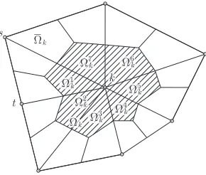
Let us partition the computational domain Ω into smoothing subdomains ¯Ω = ¯

Ω1∪Ω¯2∪...∪Ω¯N with Ωi∩Ωj =∅ if i.= j, where N is the number of finite

element nodes (including the nodes on ΓD) located in the entire computational

domain, and for every nodek= 1,· · · , N, the smoothing domain Ωk is obtained

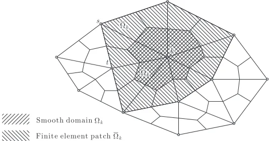
by connecting sequentially the mid-edge point to the centroid of the surrounding triangles of the node as shown in Fig. 1.

Given any strain field ε, the smoothed strain field ˆε on each smoothing domain Ωk is obtained by a nodal smoothing operation as

ˆ εk=

!

Ωk

ωk(x−xk)εdΩ,

whereωk(x) is a diagonal matrix of the smoothing functionωk(x) that is positive

and normalized to unity:

!

Ωk

ωk(x)dΩ≡1.

The smoothed strain ˆεk is a constant over the smoothing domain Ωk. For

two-dimensional elasticity problems the diagonal matrix can be chosen to beωk(x) =

diag{ωk(x),ωk(x),ωk(x)}. For simplicity the smoothing functionωk(x) is taken

as

ωk(x−xk) =

(

1/Ak, if x∈Ωk

0, otherwise

where Ak =

"

Ωk dΩ is the area of the smoothing domain Ωk. Therefore, the smoothed strain in the smoothing domain Ωk will be

ˆ εk=

1 Ak

!

Ωk

εdΩ. (9)

The SFEM is obtained by replacing in the weak form (1) the exact strain field εwith the nodally smoothed strain field ˆε. The SFEM solution ˆuh is an

approx-imation of the solution, u, to the partial differential equation of elasticity. De-note by Φi the shape function matrix for nodei, for example for two-dimensional

problems the shape function matrix

Φi(x) =

)

φi(x) 0

0 φi(x)

!k

s

t

Smo oth domain

Finit e element pat ch

!k

"

k

!k

"

!k

Figure 1: The finite element mesh and the smoothing domain Ωk.

in which φi(x) is the shape function for node i. The SFEM solution is then

expressed as

ˆ uh =

N

+

i=1

Φi(x)ˆuih, (10)

where ˆui_h ={uˆi

hx,uˆihy}T is the vector of displacements at nodei. Since the strain

field is given by the derivatives of displacement, we define the approximate strain obtained from the approximate displacements asε(ˆuh), that is

ε(ˆuh) = N

+

i=1

DΦi(x)ˆuih. (11)

For the two-dimensional elasticity problem

D= 

      

∂

∂x 0

0 ∂ ∂y ∂ ∂y

∂ ∂x



       ,

and so according to (9) by replacingεwithε(ˆuh) we obtain the smoothed strain

ˆ εk,

ˆ

εk(ˆuh) =

1 Ak

!

Ωk

and, more specifically,

ˆ

εk(ˆuh) =

1 Ak

N

+

i=1

2!

Ωk

DΦi(x)dΩ

3 ˆ ui_h

= 1 Ak

+

i∈Nk 2!

Ωk

DΦi(x)dΩ

3 ˆ uih

= 1 Ak

+

i∈Nk ˆ

Bi kuˆih,

where Nk includes all nodes in the patch ¯Ωk that is formed by the elements

sharing nodek, and

ˆ

Bik=

!

Ωk

DΦi(x)dΩ.

In the next step we will derive the stiffness matrix. The strain energy in the smoothing domain Ωkis

!

Ωk ˆ

εT_k(ˆuh)Eˆεk(ˆuh)dΩ =AkˆεTk(ˆuh)Eεˆk(ˆuh)

= 1 Ak

+

i∈Nk +

j∈Nk ˆ

uiT_h (ˆuh) ˆBkiTEBˆ j kuˆ

j h.

Therefore, the local stiffness matrix associated with nodekis obtained as

ˆ Kij(k)=

1 Ak

ˆ

BiT k EBˆ

j

k, (13)

and the global stiffness matrix for SFEM will be

ˆ Kij =

N

+

k=1

ˆ Kij(k).

The entries (in sub-vectors of nodal forces) of the force vector ˆf in the right hand side of the algebraic system can be simply expressed as

ˆ

f_i = +

k∈Nk ˆ

f_i(k). (14)

The above integration is also performed by a summation of integrals over smooth-ing domains; hence, ˆfi is an assembly of nodal force vectors at the surrounding

nodes of node k,

ˆ f_i(k)=

!

Ω(k)

Φi(x)bdΩ +

!

Γt(k)

Note that the force vector obtained in SFEM is the same as the one in FEM, if the same order shape functions is used. This simplifies the implementation of SFEM. In the Appendix, we give the implementation of SFEM with linear triangle elements in detail.

In the sequel we will give some properties of SFEM. Lemma 1 gives the orthogonality property for SFEM [15].

Lemma 1 For any compatible strain field ε(ˆuh) = Duˆh obtained by (11) on a finite element mesh Th, and the smoothed strain ˆε(ˆuh) obtained by (12) on the same mesh, we have the orthogonality property:

!

Ω

εT(ˆuh)Eˆε(ˆuh)dΩ =

!

Ω

ˆ

εT(ˆuh)Eˆε(ˆuh)dΩ. (15)

Proof We note that ˆε(ˆuh) is a piecewise constant function over the whole

domain. Equation (15) can be easily proven by relying on equation (12) and the fact thatEˆεk(ˆuh) is constant over Ωk, so that the left hand side is a sum of the

cross inner product

!

Ω

εT(ˆuh)Eˆε(ˆuh)dΩ = N

+

k=1

!

Ωk

εT(ˆuh)Eεˆk(ˆuh)dΩ

=

N

+

k=1

2!

Ωk

εT(ˆuh)dΩ

3

Eεˆk(ˆuh)

=

N

+

k=1

AkˆεTk(ˆuh)Eˆεk(ˆuh)

= !

Ω

ˆ

εT(ˆuh)Eˆε(ˆuh)dΩ. (16)

With the above orthogonality we can obtain other properties of SFEM.

Remark 1

The strain energy of the SFEM solution computed with the smoothed strain in

V_{h always bounds the strain energy obtained with the compatible strain in} V_h

from below:

!

Ω

ˆ

εT(ˆuh)Eˆε(ˆuh)dΩ≤

!

Ω

Proof We have

0≤

!

Ω

4

εT(ˆuh)−ˆεT(ˆuh)

5

E(ε(ˆuh)−ˆε(ˆuh)) dΩ

= !

Ω

εT(ˆuh)Eε(ˆuh)dΩ +

!

Ω

ˆ

εT(ˆuh)Eεˆ(ˆuh)dΩ−2

!

Ω

εT(ˆuh)Eˆε(ˆuh)dΩ

= !

Ω

εT(ˆuh)Eε(ˆuh)dΩ−

!

Ω

ˆ

εT(ˆuh)Eεˆ(ˆuh)dΩ.

Remark 2

The strain energy of the FEM solution computed with the smoothed strain in

V_{h always bounds the strain energy obtained with the compatible strain in} V_h

from below:

!

Ω

ˆ

εT(uh)Eˆε(uh)dΩ≤

!

Ω

εT(uh)Eε(uh)dΩ. (18)

Proof Since the inequality of Remark 1 holds for any displacement on mesh

Th, we can replace ˆuh with uh, i.e. the finite element solution expressed with

the same form as (10),

uh = N

+

i=1

Φi(x)uih,

and obtain the lower bounds on the strain energy computed with FEM,

!

Ω

ˆ

εT(uh)Eˆε(uh)dΩ≤

!

Ω

εT(uh)Eε(uh)dΩ.

Theorem 1 The smoothed strain energy of SFEM bounds the strain energy of FEM from above:

!

Ω

εT(uh)Eε(uh)dΩ≤

!

Ω

ˆ

εT(ˆuh)Eˆε(ˆuh)dΩ. (19)

Proof The weak form for FEM is

!

Ω

εT(uh)Eε(v)dΩ =

!

Ω

bTvdΩ + !

ΓN

tTvdΓ ∀v∈V_h,

after choosingv=uh into the above equation, we have

!

Ω

εT(uh)Eε(uh)dΩ =

!

Ω

bTuhdΩ +

!

ΓN

Both FEM and SFEM have the same right hand side as (14) in the discrete form when the same shape function is used on meshTh, then with the finite element

solution uh as the test function to SFEM we get

!

Ω

ˆ

εT(ˆuh)Eεˆ(uh)dΩ =

!

Ω

bTuhdΩ +

!

ΓN

tTuhdΓ,

By comparing the above two equations, we have

!

Ω

εT(uh)Eε(uh)dΩ =

!

Ω

ˆ

εT(ˆuh)Eˆε(uh)dΩ.

In a similar way used for the derivation of equation (16), we can omit the hat of ˆ

ε(uh) on the right hand side of the above equation, and obtain

!

Ω

ˆ

εT(ˆuh)Eˆε(uh)dΩ =

!

Ω

ˆ

εT(ˆuh)Eε(uh)dΩ,

then, from the two equations above, we get

!

Ω

εT(uh)Eε(uh)dΩ =

!

Ω

ˆ

εT(ˆuh)Eε(uh)dΩ. (20)

With the following derivation

0≤

!

Ω

4 ˆ

εT(ˆuh)−εT(uh)

5

E(ˆε(ˆuh)−ε(uh))dΩ

= !

Ω

ˆ

εT(ˆuh)Eˆε(ˆuh)dΩ +

!

Ω

εT(uh)Eε(uh)dΩ−2

!

Ω

ˆ

εT(ˆuh)Eε(uh)dΩ

= !

Ω

ˆ

εT(ˆuh)Eˆε(ˆuh)dΩ−

!

Ω

εT(uh)Eε(uh)dΩ,

and remarking that the last step in the above equation is obtained according to equation (20), we obtain an upper bound on the energy norm of the solution by FEM as

!

Ω

εT(uh)Eε(uh)dΩ≤

!

Ω

ˆ

εT(ˆuh)Eˆε(ˆuh)dΩ.

Let us set

ZP = !

Ω

ˆ

εT(ˆuh)Eˆε(ˆuh)dΩ;

ZD= !

Ω

ˆ

εT(ˆuD_h)Eˆε(ˆuD_h)dΩ; and

ZI = !

Ω

ˆ

εT(ˆuh)Eˆε(ˆuDh)dΩ.

Now we have the final formulations for the quantities appearing in (8) that are needed to compute upper and lower bounds on linear outputs by SFEM.

4

Numerical examples

We illustrate the effectivity of the proposed method on two numerical examples. Linear triangle finite element approximations are used for both primal and dual problems. Uniform mesh refinement is used in all examples to illustrate the bounding property with respect to the mesh size. Since the two examples satisfy homogeneous essential boundary conditions, uP is exactly u in the previous equations, so we will omit the superscriptP in the equations of this section.

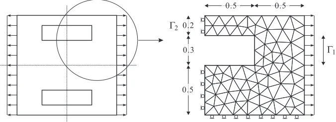
The first example is a square elastic body with two rectangular holes, under the assumption that the body is in plane stress state as shown in Fig. 2. A uniformly distributed force, p= 1, is applied on the left and right sides of the body. The non-dimensionalized Young modulus is 1.0 and Poisson ratio is 0.3. Since the geometry and load conditions in this problem are symmetric with respect to both the x- and y-axes, we only use a quarter of the body for the finite element model. Two outputs are considered in this example. The first one

!1

0.5 0.5

0.5 0.3 0.2

!2

is the average normal displacement over the boundary Γ1,

ℓO₁(u) = !

Γ1

uTndΓ,

in which n is the unit outward normal to the boundary; the second one is the reaction force on boundary Γ2,

ℓO₂(u) = !

Γ2

nT (N σ(u)) dΓ,

where

N =

)

n1 0 n2

0 n2 n1

* ,

andn1 and n2 are the components ofn. The initial (coarse) mesh with respect

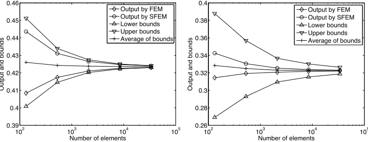
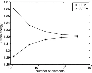
to mesh size H is plotted in Fig. 2. The uniformly refined meshes are based on mesh sizes H/2, H/4, H/8, and H/16 respectively. The results for ℓO₁(u) and ℓO₂(u) including the outputs calculated by FEM and SFEM, the upper and lower bounds, and the average of the upper and lower bounds are plotted in Fig. 3. From equation (8) the average of bounds is actually the average of the outputs by FEM and SFEM, that is 1₂(ℓO(uh) +ZI) = ₂1(ℓO(uh) +ℓO(ˆuh)). We also

plot the strain energies computed by FEM and SFEM in both primal and dual problems for the two outputs in Figs. 4-5. We will analyze the effectivity of the bounds by a measure given at the end of this section.

102 103 104 105

0.39 0.4 0.41 0.42 0.43 0.44 0.45 0.46

Number of elements

O

u

tp

u

t

a

n

d

b

o

u

n

d

s

Output by FEM Output by SFEM Lower bounds Upper bounds Average of bounds

102 103 104 105

0.26 0.28 0.3 0.32 0.34 0.36 0.38 0.4

Number of elements

O

u

tp

u

t

a

n

d

b

o

u

n

d

s

Output by FEM Output by SFEM Lower bounds Upper bounds Average of bounds

Figure 3: The upper and lower bounds on the displacement outputℓO₁(u) (left) and the reaction outputℓO₂(u) (right).

102 103 104 105 1.28

1.29 1.3 1.31 1.32 1.33 1.34 1.35 1.36 1.37

Number of elements

St

ra

in

e

n

e

rg

y

FEM SFEM

Figure 4: The strain energies computed by FEM and SFEM in the primal prob-lems for the first two outputs.

102 103 104 105

0.18 0.19 0.2 0.21 0.22

Number of elements

St

ra

in

e

n

e

rg

y

FEM SFEM

102 103 104 105

0.3 0.35 0.4 0.45 0.5 0.55

Number of elements

St

ra

in

e

n

e

rg

y

FEM SFEM

Crack tip

10

30

5

Crack tip

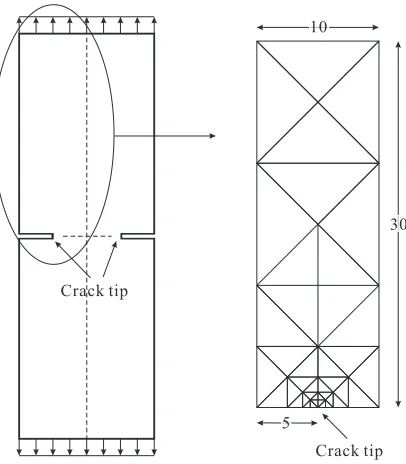
Figure 6: A double edge-cracked elastic plate subject to a uniform tensile stress: just a quarter of the structure is used for the finite element modeling. The finite element mesh shown in the right figure is the initial mesh with 41 elements.

the so-calledJ-integral, which is defined in the domain integral form as

ℓO₃(u) = 1₂ !

Ωχ uT_x

)

Q−∂χ

∂xD˜ *

uxdΩ, (21)

where the integration domain Ωχ contains the crack tip,

ux= (

∂ux

∂x, ∂uy

∂x , ∂ux

∂y , ∂uy

∂y 6T

,

χ is the weight function equal to one at the crack tip and vanishing on the boundary of Ωχ, Q and ˜D are matrices containing the elastic parameters and

the weight function χ, refer to the appendix in [19]. From equation (21) we see that J-integral is a quadratic function of the displacement, to express the following equations clearly we useJ(u,u) to expressℓO

3(u), so that we have

ℓO₃(u)−ℓO₃ (uh) =J(u,u)−J(uh,uh)

=J(u−uh,u−uh) + 2J(u−uh,uh). (22)

In [19] it was found that

J(u−uh,u−uh)≤ηχ*u−uh*2

=ηχ&*u*2− *uh*2

'

≤ηχ&*uDh*2− *uh*2

'

Crack tip 5

5 5

"#

Figure 7: A 5×5 integral domain Ωχis arranged for evaluation of theJ-integral.

whereηχ is a computable quantity related to elasticity coefficients and toχ. For

the second term in equation (22),

J(u−uh,uh) =J(u,uh)−J(uh,uh), (24)

we noteJ(u,uh) is a linear function of u, thus with bounding formulations for

the linear output (8), we can compute the upper and lower bounds onJ(u,uh),

that is

ℓ−≤J(u,uh)≤ℓ+.

Let Q= η&

*uD_h*2_{− *u} h*2

'

in equation (23), and consider the equations (22), (23), (24) and (8). The upper and lower bounds formulations for theJ-integral are summarized as follows:

J+=ZI+Q+ %

(Z − *uh*2)

&

ZD_{− *u}D h*2

' ,

J−=ZI−Q−%(Z − *uh*2)

&

ZD_{− *u}D h*2

' .

(25)

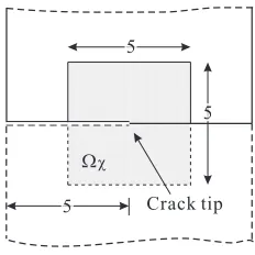
In this example, due to the symmetry of the problem, we only use one quarter of the plate for the finite element modeling. We use a 5 by 5 square area surrounding the crack tip as the support, Ωχ, of the weighting functionχ, see

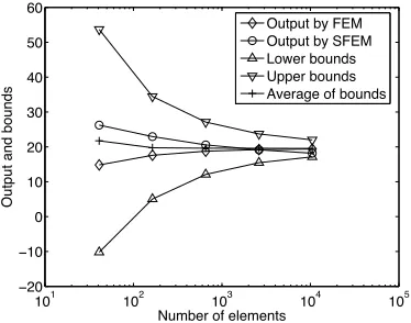
Fig. 7. We should note that the J-integral gets a contribution from the entire half plate, but we only use a quarter of the plate for the finite element model, so we need to multiply the outputs computed by this finite element model by two, including theJ-integral and all terms on the right hand side of equation (25). There is no such issue for the outputs in the previous example. The bounding results computed are plotted in Fig. 8, where the formulation of average of the bounds is different from that of the first two linear outputs, from (25) we can see the average is ZI_{, that is Z}I _{= ℓ}O_(ˆu

h) = J(ˆuh,uh). The strain energies

computed by FEM and SFEM in the primal and dual problems are plotted in Fig. 9.

We introduce the relative half bound gap given in [9]

ρG= 1₂

101 102 103 104 105 −20

−10 0 10 20 30 40 50 60

Number of elements

O

u

tp

u

t

a

n

d

b

o

u

n

d

s

Output by FEM Output by SFEM Lower bounds Upper bounds Average of bounds

Figure 8: The upper and lower bounds on the J-integral ℓO₃ (u).

101 102 103 104 105

610 620 630 640 650 660 670

Number of elements

St

ra

in

e

n

e

rg

y

FEM SFEM

101 102 103 104 105

0 2 4 6 8 10 12 14 16

Number of elements

St

ra

in

e

n

e

rg

y

FEM SFEM

as a measure of the accuracy of the bounds. It is certainly an upper bound on the relative error between the average of the bounds and the exact outputℓ(u). Since the exact output ℓ(u) is not known for the examples, we use the average of the bounds calculated with a finer mesh of mesh sizeH/16 instead. Thus a computable measure of the accuracy of the bounds is given by

ρG =

ℓ+−ℓ− ℓ∗+_+ℓ∗− ,

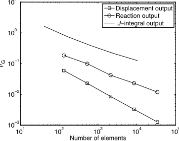
whereℓ∗+ and ℓ∗− are the upper and lower bounds calculated in the mesh with mesh size H/16. Fig. 10 shows the convergence results of ρG for the three

outputs. The convergence rates do not attain the optimal converge rate of 1, because there are singularities (corners and crack tip) in both the two examples. The convergence rate for the displacement output, 0.7, is the biggest, and the relative bound gap is the smallest. The convergence rates for the stress output and the J-integral are 0.5 and 0.46, respectively. The convergence rate for the J-integral is the smallest, because the approximate solutions are dominated by a singularity caused by the crack, which affects the convergence rate much more than the effect caused by corners in the first example. The relative half bound gap for theJ-integral is the largest in the three outputs, the main reason being that the difference between the strain energies computed by FEM and SFEM in the dual problem is very large, see the left figure in Fig. 9. The exact strain energy of the dual problem is about 6, but the strain energy computed by SFEM has trouble converging to this value and only provides an upper bound. This is an issue that sometimes arises with SFEM, although it does not happen often. The strain energies computed by SFEM in the primal problem for theJ-integral and in both primal and dual problems for other outputs in the first example are very effective.

101 102 103 104 105

10−3 10−2 10−1 100 101

Number of elements

ρG

Displacement output Reaction output J₋integral output

5

Conclusions and discussion

We have examined SFEM with linear triangle elements and extended it to com-pute upper and lower bounds on general linear outputs of displacements in elas-ticity. In the examples we have considered, SFEM behaves like an equilibrium method and the strain energy converges to the true strain energy from above. We also find that in some cases the energy norm of the solution by SFEM does not reach the exact strain energy, as shown in the right side of figure Fig. 9, but can be used as an upper bound indicator. However, in most cases SFEM really gives a convergent upper bound on the strain energy and, consequently, also gives convergent upper and lower bounds on general linear outputs. One of the most important advantages of bounds computation by SFEM is that they are very easy to implement, as this simply requires a modification of a few lines of our underlying finite element code to implement SFEM. This is an advantage over the equilibrium method to obtain upper bounds. We also note that many a posteriori error estimates proposed in literature are an order of magnitude more expensive to compute than the finite element solution. In contrast, the computation of upper bounds using SFEM is only about as expensive as solv-ing the regular finite element problem. Further research will be on solvsolv-ing the convergence problem of SFEM, and extending it to solve inelasticity problems as done by Ledev`eze and his coworkers [20, 21].

Acknowledgements

This work was performed while the first author was visiting the Chair of Mod-elling and Scientific Computing (CMCS), Institute of Analysis and Scientific Computing (IACS), ´Ecole Polytechnique F´ederale de Lausanne (EPFL), and was supported by the National Natural Science Foundation of China under grant number 10872146.

Appendix

For two-dimensional elasticity problems, the relation between displacement,u=

{ux, uy}T, and strain, ε(u), is ε(u) =Du,

ε(u)≡



      

      

∂ux

∂x ∂uy

∂y ∂uy

∂x +

∂ux

∂y 

      

      

= 





ε11(u)

ε22(u)

2ε12(u)







and the corresponding stress according to σ = Eε(u) is specifically expressed as σ≡    σ11 σ22 σ12    =  

λ+ 2µ λ 0

λ λ+ 2µ 0

0 0 µ



 





ε11(u)

ε22(u)

2ε12(u)





 ,

whereλ and µare Lame’s constants, µ= ₂₍₁₊E_ν), and λ= _(1+νEν_)(1−2ν) for plane strain problem,λ= ₁₋Eν_ν2 for plane stress problems.

Let the approximate finite element solution of displacement be

uh = N

+

i=1

Φi(x)uih,

where Φi(x) is the nodal shape function containing x and y components. For

implementation we usually first construct the elemental stiffness matrix and then assembly them to global stiffness matrix. We define the displacement vector on element T ∈ Th to be uh T = {u1x, u1y, u2x, u2y, u3x, u3y}T, where the subscript T

denotes elementT. Then the displacement of element T can be expressed as

uh T(x) =

)

φT1 0 φT2 0 φT3 0

0 φT1 0 φT2 0 φT3

* uhT,

whereφT1,φT2 andφT3 are the shape functions in elementT, and with (26) the

approximate strain in elementT is obtained as

εh T =Ruh T, (27)

in which R=         ∂φT1 ∂x 0 ∂φT2 ∂x 0 ∂φT3 ∂x 0

0 ∂φT1

∂y 0 ∂φT2 ∂y 0 ∂φT3 ∂y ∂φT1 ∂y ∂φT1 ∂x ∂φT2 ∂y ∂φT2 ∂x ∂φT3 ∂y ∂φT3 ∂x         , (28)

the strain energy in elementT is then obtained by

!

T

σT_{h T}εh TdΩ =ATuTh TRTERuh T,

whereAT is the area of elementT. Therefore the element stiffness matrix is

With the following equation for computing the derivatives of the shape functions the implementation of the local stiffness matrix is much simplified,

∇ΦT =

1 2AT





y1−y3 x3−x2

y3−y1 x1−x3

y1−y2 x2−x1





= 



1 1 1 x1 x2 x3

y1 y2 y3

  −1  0 0 1 0 0 1  .

The construction of the elemental stiffness matrix in FEM is based on the element, while the construction of the local stiffness matrix for SFEM is based on the smoothing domain. The local stiffness matrix will involve contributions from all nodes that belong to the patch. For example, the smoothing domain Ωk is in the patch ¯Ωk, see Fig. 1. The smoothed strain ˆεk is in fact an area

weighted average strain that is

ˆ εk=

1 Ak

!

Ωk

ε(x)dΩ

= 1 Ak Mk + I=1 ! ΩI k

εI_k(x)dΩ,

in which Mk is the number of elements that contain node k. For example,

the smoothing domain k in Fig. 11 has 7 subdomains; ΩI_k is a subdomain of domaink, and εI_k(x) is the strain in subdomain ΩI

k. In the above equation, we

do not use small i but use capital I to represent the subdomain label, in this way we will distinguish the following equations from the ones in Section 3: there the formulation is related to node i, while here the formulation is related to subdomainI. The strain energy in the smooth subdomaink

!

Ωk ˆ

εT_kEˆεkdΩ =AkˆεTkEˆεk

= 1 Ak >_M k + I=1 ! ΩI k

εIT_k (x)dΩ ? E >_M k + J=1 ! ΩJ k

εJ_k(x)dΩ ?

.

Because the shape functions are linear, εI_k(x) is constant over each element, and is certainly constant over ΩI

k for it being one part of an element, thus the

arguments in the above equation are omitted, and it is in a more simplified form

!

Ωk ˆ

εT_kEˆεkdΩ =

1 Ak Mk + I=1 Mk + J=1

AI_kAJ_kεIT_k EεJ_k, (29)

forI, J = 1,· · · ,Mk, andεI_k and εJ_k are in the form of (27), that is,

εI_k=RI_kuˆI_h;

s

t

!k

"

k

!1k

!k2

!3k

!k4

!5k

!k6

!k7

!k

Figure 11: Illustration of patch ¯Ωk, smoothing domain Ωk, and smoothing

sub-domains ΩI_k.

whereRI_k andRJ_k are in the form of (28). Substituting (30) into (29) we obtain

!

Ωk ˆ

εT_kEεˆkdΩ =

1 Ak

Mk +

I=1 Mk +

J=1

AI_kAJ_kuˆIT_h RIT_k ERJ_kuˆJ_h.

Then we obtain the entries of local stiffness matrix in Ωk

ˆ

K_{I}{J}(k)=

AI kAJk

Ak

RIT_k ERJ_k. (31)

Since the smoothing domain is formed by connecting the central points of ele-ment edges to the centroids of eleele-ments, we see that AI

k is 1/3 of the element

area, SI

k, for example, area of Ω1k is 1/3 of area of the element kst in Fig. 11;

andAkis 1/3 of the sum of area of all elements in ¯Ωk, therefore (31) is rewritten

as

ˆ

K{I}{J}(k)=

SI kSkJ

3@Mk

l=1 Slk

RIT_k ERJ_k. (32)

As compared with (13) that is a 2×2 matrix, (32) is a matrix that contains 36 entries. The Matlab code for construction of the local stiffness matrix and assembly of the global stiffness matrix is listed as follows:

for k = 1:size(coor,1)

[r,c,v] = find(ele == k); S = [];

for m = 1:size(r,1)

S(m) = det([1,1,1;(coor(ele(r(m),:),:))’])/2; end

vertices = coor(ele(r(I),:),:);

II = 2*ele(r(I),[1,1,2,2,3,3])-[1,0,1,0,1,0]; PhiGrad = [1,1,1;vertices’]\[zeros(1,2);eye(2)]; RI = zeros(3,6);

RI([1,3],[1,3,5]) = PhiGrad’; RI([3,2],[2,4,6]) = PhiGrad’; for J = 1:size(r,1)

vertices = coor(ele(r(J),:),:);

JJ = 2*ele(r(J),[1,1,2,2,3,3])-[1,0,1,0,1,0]; PhiGrad = [1,1,1;vertices’]\[zeros(1,2);eye(2)]; RJ = zeros(3,6);

RJ([1,3],[1,3,5]) = PhiGrad’; RJ([3,2],[2,4,6]) = PhiGrad’;

K(II,JJ) = K(II,JJ) + 1/3/SumS*S(I)*S(J)*RI’*E*RJ; end

end end

In the program,coorandeleare the data of nodes coordinates and node num-bers of vertices, respectively. II and JJ are the indices expressed by {I} and

{J}in the equations, respectively. The other part for SFEM including assembly of the right hand side and incorporation of Dirichlet conditions is the same as the procedure used in FEM, see [22].

References

[1] P. Ladev`eze, D. Leguillon, Error estimate procedure in the finite element method and applications, SIAM J. Numer. Anal. 20: 485-509, 1983.

[2] R.E. Bank, A. Weiser, Some a posteriori error indicators for elliptic partial differential equations, Math. Comput. 44: 283-301, 1985.

[3] M. Ainsworth, J.T. Oden, A posteriori error estimation in finite element analysis, Comput. Methods Appl. Mech. Engrg., 142: 1-88, 1997.

[4] P. Destuynder, B. M´etivet, Explicit error bounds in a conforming finite element method, Math. Comput. 68: 1379-1396, 1999.

[5] M. Paraschivoiu, J. Peraire, A.T. Patera, A posteriori finite element bounds for linear-functional outputs of elliptic partial differential equations. Com-put. Methods Appl. Mech. Engrg., 150: 289-312, 1997.

[7] S. Prudhomme, J.T. Oden, On goal-oriented error estimation for elliptic problems: application to the control of pointwise errors, Comput. Methods Appl. Mech. Engrg., 176: 313-331, 1999.

[8] J.T. Oden, S. Prudhomme, Goal-oriented error estimation and adaptivity for the finite element method. Comput. Math. Appl., 41: 735-756, 2001.

[9] N. Par´es, J. Bonet, A. Huerta, J. Peraire, The computation of bounds for linear-functional outputs of weak solutions to the two-dimensional elasticity equations. Comput. Methods Appl. Mech. Engrg., 195: 406-429, 2006.

[10] B.F. de Veubeke, Displacement and equilibrium models in finite element method. In O.C. Zienkiewicz, G.S. Holister (Eds.), Stress Analysis, John Wiley and Sons, Chichester, 145–197, 1965.

[11] D.N. Arnold, Mixed finite element methods for elliptic problems, Comput. Methods Appl. Mech. Engrg., 82: 1-88, 1990.

[12] D.N. Arnold, R. Winther, Mixed finite elements for elasticity, Numer. Math., 92: 401-419, 2002.

[13] R.H. Gallagher, Finite element structural analysis and complementary en-ergy, Finite Elem. Anal. Des., 13: 115-126, 1993.

[14] G.R. Liu, K. Zaw, Y.Y. Wang, B. Deng, A novel reduced-basis method with upper and lower bounds for real-time computation of linear elascity problems, Comput. Methods Appl. Mech. Engrg., 198: 269-279, 2008.

[15] G.R. Liu, G.Y. Zhang, Upper bound solution to elasticity problems: A unique property of the linearly conforming point interpolation method (LC-PIM), Int. J. Numer. Meth. Engrg, 74: 1128-1161, 2008.

[16] G.R. Liu, H. Nguyen-Xuan, T. Nguyen-Thoi, X. Xu, A novel Galerkin-like weakform and superconvergent alpha finite element method for mechanics problems using triangle meshes, J. Comput. Phys., 228: 4055-4087, 2009.

[17] J.S. Chen, C.T. Wu, S. Yoon, Y. You, A stabilized conforming nodal inte-gration for Galerkin mesh-free methods. Int. J. Numer. Meth. Engrg., 50: 435-466, 2001.

[18] H. Nguyen-Xuan, S. Bordas, H. Nguyen-Dang, Smooth finite element meth-ods: Convergence, accuracy and properties, Int. J. Numer. Meth. Engrg, 74:175-208, 2008.

[20] P. Ladev`eze, J.P. Pelle, Mastering calculations in linear and nonlinear me-chanics, Springer, 2005.

[21] L. Chamoin L, P. Ladev`eze, Bounds on history-dependent or independent local quantities in viscoelasticity problems solved by approximate methods. Int. J. Numer. Meth. Engrg., 71: 1387-1411, 2007.