Fixed and random coefficient time series

by

B ar r y G. Quinn

A thesis submitted to the Australian National University

for the degree of Doctor of Philosophy

P R E F A C E

Most of the results in Chapter 2 have appeared in Quinn (1980), and are multivariate generalisations of results obtained in collaboration with

Professor E.J. Hannan which appear in Hannan and Quinn (1979). Chapters 4 through 6 contain the results of work carried out in conjunction with Dr D.F. Nicholls, from which several papers have been considered for

publication. Except where otherwise stated, the work presented in this thesis is my own.

A C K N O W L E D G E M E N T S

There are many people I would like to thank for making the three years of my PhD so enjoyable. First and foremost, I am indebted to my supervisors Professor E.J. Hannan and Dr D.F. Nicholls, whose knowledge and expertise contributed greatly to the work presented in this thesis. The academic environment created by the members of and visitors to the Statistics

Departments of the Research School of Social Sciences and of the Faculty of Economics has made study and research both stimulating and profitable.

ABSTRACT

Linear modelling of data has been a major concern in time series for many years. One of the last outstanding problems has been the determination of the order of a model once a class of models has been decided upon. In Chapter 2 automatic criteria for the determination of the order of a multivariate autoregression are discussed. Via a law of the iterated logarithm for martingales, it is shown under what conditions an automatic criterion of a certain type is strongly consistent for the true order of the autoregression.

The theory of linear models is now essentially complete. Thus interest has shifted towards developments in non-linear modelling. The remainder of the thesis is concerned with non-linear models, and especially non-linear generalisations of the autoregressive models. In Chapter 3 a simple

bilinear model reveals some of the complexities encountered when non-linear modelling is considered. Conditions are found for the existence of strictly stationary solutions to the model equations, and for the invertibility of such models. The methods are then extended to obtain conditions for the existence of strictly stationary solutions to simple random coefficient models.

In Chapter 4 a class of multivariate random coefficient autoregressive models is introduced. Conditions are found for the existence of second order stationary solutions and for the stability of such models. In

Chapters 5 and 6, two-stage least squares and maximum likelihood estimation procedures, respectively, are proposed. In each case the estimates are shown to be strongly consistent and to satisfy a central limit theorem. In Chapter 7, simulated processes are estimated using the techniques of Chapters

C O N T E N T S

PREFACE ... ACKNOWLEDGEMENTS ... ABSTRACT ... CHAPTER 1: INTRODUCTION ... 1.1. Introduction ... 1.2. Kronecker Notation and Some Matrix Results

1.3. General Notation ... CHAPTER 2: ORDER DETERMINATION FOR AUTOREGRESSIVE PROCESSES .. ..

2.1. Introduction ... 2.2. A Decomposition of ... 2.3. The Asymptotic Behaviour of 4y(k) ... 2.4. Asymptotic Behaviour of the Minimum AIC Procedure 2.5. Strongly Consistent Procedures ... 2.6. Simulations ... CHAPTER 3: STATIONARITY AND INVERTIBILITY OF SIMPLE BILINEAR MODELS

3.1. Introduction ... 3.2. Ergodic Theory ... 3.3. Existence of an F^-Measurable Strictly Stationary

Solution to (3.1.1) ... 3.4. Invertibility ... 3.5. A Simple Random Coefficient Autoregressive Model CHAPTER 4: RANDOM COEFFICIENT AUTOREGRESSIVE MODELS ...

4.1. Introduction ... 4.2. Existence of a Singly-Infinite Stationary Solution

to (4.1.1) ... 4.3. Existence of a Doubly-Infinite Stationary Solution

to (4.1.1) ... 4.4. The Case Where (M

®

M+C) has a Unit Eigenvalue 4.5. Stability of Processes Generated by (4.1.1) From t -

1

. . . .

4.6. Strict Stationarity of the Solution {X(t)} to

(4.1.1) ...

CHAPTER 5: LEAST SQUARES ESTIMATION OF RANDOM COEFFICIENT

AUTOREGRESSIONS ... 79 5.1. Introduction ... 79 5.2. The Estimation Procedure ... 80 5.3. Strong Consistency and the Central Limit Theorem 82 CHAPTER 6: MAXIMUM LIKELIHOOD ESTIMATION OF RANDOM COEFFICIENT

AUTOREGRESSIONS ... 95 6.1. Introduction ... 95 6.2. The Maximum Likelihood Procedure ... 96

/S. A ^2

6.3. The Strong Consistency of y/v5 ... 99 6.4. The Central Limit Theorem ... 107 CHAPTER 7: ESTIMATION OF RANDOM COEFFICIENT AUTOREGRESSIONS - SOME

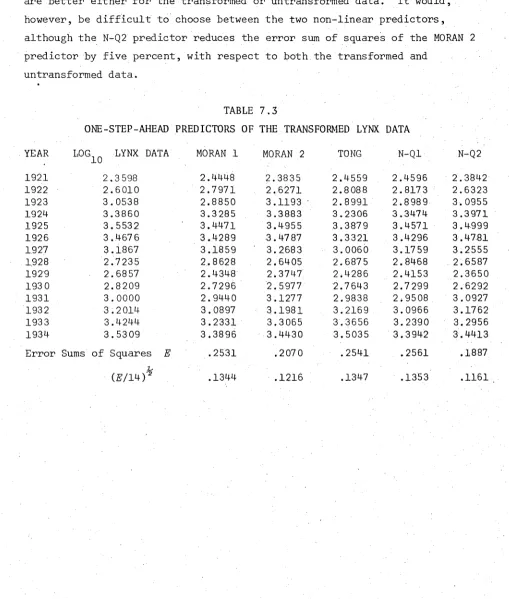
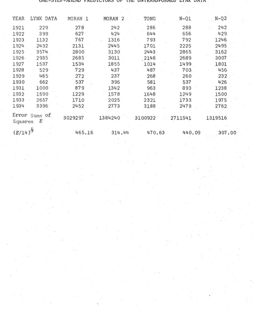
NUMERICAL RESULTS ... Ill 7.1. Introduction ... Ill 7.2. The Method of Simulation and Estimation... 112 7.3. First and Second Order Random Coefficient

I N T R O D U C T I O N

1.1.

I n t r o d u c t i o n

Much of the recent time series literature has been concerned with the modelling of data using time-domain techniques. Linear models have

frequently been used since, by the Wold decomposition theorem, a linearly purely deterministic second order stationary process (X(t)} has a linear decomposition in terms of a second order stationary uncorrelated time series

(e(t)} . It has been usual, however, for theoretical purposes, to assume that (e(t)} is an independent process, although Hannan and Heyde (1972) have shown that least squares linear prediction is equivalent to least

squares non-linear prediction as long as {c(t)} is a sequence of martingale differences. Much of the recent theory of linear models,

therefore, has made this assumption and the relaxed condition has been seen in many circumstances not to affect seriously the theory which was obtained under the more restrictive independence assumptions. Of course, the general linear model involves an infinite number of parameters, so that finite

parameter models, and in particular the autoregressive moving-average (ARMA) models, have played a dominant role in the linear modelling of data.

Many of the theoretical problems, such as estimation, have long since been solved for the linear models, and during the last decade a certain amount of attention has been focused on obtaining more efficient estimation techniques for the ARMA models, on small sample investigations and on

determining the orders associated with these models,while several attempts have been made to develop and implement a practical class of non-linear models. These last two problems are the main concern of this thesis.

b y A k a ik e ( 1 9 7 8 ) , Shw arz ( 1 9 7 8 ) , R i s s a n e n ( 1 9 7 8 ) a n d Hannan and Quinn ( 1 9 7 9 ) i n a r e s p o n s e t o a n e g a t i v e f e a t u r e o f t h e minimum AIC p r o c e d u r e . S h i b a t a ( 1 9 7 6 ) h a s shown t h a t i f d a t a t r u l y come fro m a n a u t o r e g r e s s i o n , t h e n t h e r e i s a n o n - z e r o p r o b a b i l i t y t h a t t h e minimum AIC p r o c e d u r e a s y m p t o t i c a l l y o v e r e s t i m a t e s t h e t r u e o r d e r , t h a t i s , t h e minimum AIC p r o c e d u r e i s n o t w e a k l y c o n s i s t e n t . Hannan and Quinn h a v e o b t a i n e d t h e c o n d i t i o n s u n d e r w h ic h a n a u t o m a t i c p r o c e d u r e o f t h e AIC t y p e i s s t r o n g l y c o n s i s t e n t , and t h e m u l t i v a r i a t e g e n e r a l i s a t i o n o f t h e i r r e s u l t and t h e r e s u l t o f S h i b a t a i s t h e

s u b j e c t o f C h a p t e r 2.

A c l a s s o f n o n - s p e c i f i c n o n - l i n e a r m o d e l w h ic h h a s b e e n d e v e l o p e d i n r e c e n t y e a r s i s t h e b i l i n e a r m o d e l , i n t r o d u c e d i n t h e e n g i n e e r i n g l i t e r a t u r e and r e c e n t l y c o n s i d e r e d i n m ore g e n e r a l i t y by G r a n g e r and A n d e r s e n ( 1 9 7 8 a ) a s a v i a b l e e x t e n s i o n o f t h e ARMA t i m e s e r i e s m o d e l s . A num ber o f r e s u l t s h a s becom e a v a i l a b l e f o r s e v e r a l s u b c l a s s e s o f t h e b i l i n e a r m o d e l s an d a f u n d a m e n t a l p r o b le m i s s o l v e d i n t h i s t h e s i s f o r t h e s i m p l e ( o n e - p a r a m e t e r ) m o d e l s : o f t e n when a m o d e l i s p r o p o s e d i t i s a ssu m ed t h a t t h e r e i s a

s t a t i o n a r y s o l u t i o n t o t h e m o d e l e q u a t i o n , a n d c e r t a i n moments a r e c a l c u l a t e d by f o r m a l l y m a n i p u l a t i n g t h i s e q u a t i o n . H ow ever, t h e e x i s t e n c e o f a

s t a t i o n a r y s o l u t i o n m u st b e shown b e f o r e t h i s t r e a t m e n t beco m es r i g o r o u s . C o n d i t i o n s a r e t h u s o b t a i n e d f o r t h e e x i s t e n c e o f s t a t i o n a r y s o l u t i o n s , and a s i m i l a r m eth o d i s u s e d t o s o l v e t h e p r o b l e m o f i n v e r t i b i l i t y . We

i n c i d e n t a l l y f i n d c o n d i t i o n s f o r t h e e x i s t e n c e o f s t a t i o n a r y s o l u t i o n s t o u n i v a r i a t e f i r s t o r d e r random c o e f f i c i e n t a u t o r e g r e s s i v e m o d e l e q u a t i o n s .

The t h e o r y w h ic h h a s b e e n d e v e l o p e d f o r a u t o r e g r e s s i v e m o d e ls was o b t a i n e d i n a much s i m p l e r f a s h i o n t h a n t h a t f o r t h e g e n e r a l l i n e a r t i m e s e r i e s m o d e l . C o n s e q u e n t l y i t h a s b e e n n a t u r a l t o c o n s i d e r n o n - l i n e a r g e n e r a l i s a t i o n s o f t h e a u t o r e g r e s s i v e m o d e l s . Tong ( 1 9 7 8 ) h a s i n t r o d u c e d a c l a s s o f m o d e l s known a s t h e t h r e s h o l d a u t o r e g r e s s i o n s , f o r w h ic h

r e a l i s a t i o n s a r e c o n s i d e r e d a s s a t i s f y i n g d i f f e r e n t a u t o r e g r e s s i v e m o d e l s d e t e r m i n e d b y t h e v a l u e o f some p a s t d a tu m . O z a k i ( 1 9 7 8 ) h a s c o n s i d e r e d an

e x p o n e n t i a l d a m p in g o f t h e a u t o r e g r e s s i v e c o e f f i c i e n t s , t h e e x p o n e n t i a l t e r m s h a v i n g l e a s t e f f e c t when a p a s t v a l u e o f t h e t i m e s e r i e s i s l a r g e , and m ost e f f e c t when t h e v a l u e i s s m a l l . E ach o f t h e s e c l a s s e s o f m o d e l s was d e v e l o p e d t o e x p l a i n t h e n a t u r a l phenomenon known a s t h e l i m i t c y c l e , b u t t h e i r t h e o r e t i c a l t r e a t m e n t i s d i f f i c u l t , w h i l e t h e m o d e ls i n v o l v e a

the class of multivariate random coefficient autoregressions, which may be regarded as autoregressions whose coefficients are randomly perturbed in an

independent manner from time to time. Conlisk (1974, 1976) has found conditions for the stability of these processes, while Andel (1976) has investigated the problem of second order stationarity for the univariate models. The major part of this thesis is concerned with the development of a rigorous theory for these models along the lines of that obtained for the fixed coefficient autoregressions. We obtain conditions for the existence of stationary solutions to the model equations, as well as proposing and implementing two techniques for their estimation, and examining the asymptotic behaviour of the estimates obtained.

The theoretical results of this thesis will depend to a large extent on several results from the theory of probability. In particular, we shall need a certain amount of ergodic theory, the relevant results being

presented in §3.2. We shall also be utilising the theory of martingales, especially the central limit theorem of Billingsley (1961) and a law of the iterated logarithm of Stout (1970) which we state here for

reference purposes.

T H E O R E M 1.1

(Billingsley). Let

{ £ ( £ ) }

be a square-integrable stationary ergodic processj and denote by F^ the a-field generated by {$(*), W - 1), ...} . If ff(5(t)|Ft = 0 , then

2 -f' ^ 2 2

[c N] 2 Y, £>(t) j where c =£'{£(£)}., has a distribution which converges t=1

to the standard normal distribution.

T H E O R E M 1 . 2

(Stout). Under the conditions of Theorem 1.1, 9 - > N

(2c N In In n) 2 £ E,(t) = b(N) ^ where lim sup b(N) = - lim inf b(N) = 1

t=1 N N

1.2.

K r o n e c k e r N o t a t i o n a n d S o m e M a t r i x R e s u l t s

Throughout the thesis, frequent use of Kronecker (or tensor) notation will be made. This notation permits the simple solution of many matrix equations, and facilitates the simplification of certain complicated

We define firstly the Kronecker (or tensor) product of two matrices.

D E F I N I T I O N

1.2.1. Let

A

and P be

m x n

and p x q matrices

respectively. Then the Kronecker product A ® B of

B with

A

is the

mp

x

nq

matrix whose (i, j)th block is the p x q matrix .P , where

A^ .

is the (i, J)th element of

A .

Next, given any

m x n

matrix

A

, we may define an mn-component vector which has as its elements the elements of

A .

D E F I N I T I O N

1.2.2. Let

A

be an

m x

n matrix.

Then the

mn-component vector vec A is obtained from

A by stacking the columns of

A

, one on top of the other, in order, from left to right.

The results contained in the following theorem hold for any matrix products which are defined, and are stated without proof.

T H E O R E M

1.3. 1. v ec(ABC) = (Cr 0 A) vec B . 2.

tv

(AB) =

(vec

(B')) ’

vec A = (vec

B)' vec

(A1)

. 3.

(A

®

B)(C

®

D)

=

(AB)

0

(CD)

.

4.

(A

® P)"1 = 4 “1 ® P _1 ,

(A

0 P ) f =

A'

® B ’ .

The results of this theorem will be used repeatedly. In particular, the first result will be used to solve a matrix equation which appears frequently in Chapter 4, and which is solved now in more generality.

T H E O R E M

1.4.

Let V be an n x n matrix which satisfies the

equation

V = MVN’

+

G

(1.2.1)

where

A/,

N and G are given n

x

n matrices. Then if (I - N

0

M) is

invertible3 there is a unique solution V which may be obtained from

vec

V - (I - N

®

M)

^ vec

G

.

Proof. Taking the vec of each side of (1.2.1) we obtain

vec

V =

vec(MVN1)

+ vec G - N ®

M vec

V

+ vec

G

, by Theorem 1.3.1. Thus

(I -

N ®

M)

vec

V = vec

G

and

vec

V

=

(I - N

® M)"1 vec

G

. //

of

A

. Henderson and Searle (1979) have considered a vector composed of the non-redundant elements of

A

, which is defined in the following manner.

DEFINITION 1.2.3.

Let

A

be an

n

x

n

symmetric matrix. The

n(n+l)/2-component vector vech

A

(the "vector-half" of

A

) is obtained from

A

by stacking those parts of the columns of

A

, on and below the main diagonal, one on top of the other in order from left to right.

For symmetric matrices

A

, it is possible to obtain by linear

transformations the vector vec

A

from the vector vech

A

, and

vice versa

, which is shown in the following theorem.

THEOREM 1.5.

There exist eonstant

n(n+l)/2 x

n

matrices

H

for which

vech

A = H

vec

A and

vec

A - K'

vech

A for any

n

n

n

J

symmetric matrix A

,

and H K' - I ,

, . .

s

n n

n(tt+l)/2

K

and

n

n

x

n

2

Proof.

Let

H

be the n(n+l)/2 x

n

matrix formed by eliminating

the {

(k-l)n+l}th

rows from

I

2 for 2 < (Z-+1)

< k < n .

Then it is easy

n

to see that vech

A - H

vec

A

, since those rows which have been eliminated

n

correspond exactly with the redundant elements of vec

A

.

The matrix

K r

reinstates the aforementioned redundant elements of

n

vec

A

, and

K

_n

is constructed by adding the { (/c-l)n+Z-}th row of T _{j o}

_Yi

2 to the {

(l-l)n+k}th

row, for 2 < (1+1)

< k S n ,

and then eliminating the former rows.

Now, letting

x

be any

n(n+l)

/2-component vector, and

X

the symmetric

n

x

n

matrix for which

x

= vech

X

, we have

H K rx = H [x'

vech j) =

H

vec

X -

vech

X

=

x .

n n

n y n

J

n

Thus

H K ’

=

I .

1 w _ .

n n

n{n+l)/2

H

As an example of the above construction we consider the case

n -

2 . The matrices and

K^

are given by

1 0 0 0 1 0 0 0

0 1 0 0 , k2 = 0 1 1 0

0 0 0 1 0 0 0 1

then

while

A =

x y

1 ZA

H

2 vec

A

-

vech

A

,

K

2 vech

A

-

vec

A

1.3. General Notation

We list below the symbols and abbreviations used in the text of this thesis.

(i) Internal Referencing

§1.2

(1.2.3) Lemma 1.2 Theorem 1.2 Theorem 1.2.3 Corollary 1.2.3 Definition 1.2.3 Table 1.2

Fig. 1.2

Section 2 of Chapter 1 Equation number 3 of §1.2 The second lemma of Chapter 1 The second theorem of Chapter 1 The third part of Theorem 1.2 The third corollary of Theorem 1.2 The third definition in §1.2

The second table in Chapter 1 The second figure in Chapter 1

(ii) Mathematical Notation

}uals by definition

is bounded almost surely

A E q u a l s

ii _{o H}

=

3

^

V**

o

II

W

‘0

~

~

'

4

-%

O

II _N „■- e - 6_{y converges almost surely to zero for all}

[image:12.557.21.544.26.820.2]

l i m s u p X

n n l i m s u p X, n * 00 k > n

l i m i n f X

n n l i m i n f X. nx»

(ft, F , P ) A p r o b a b i l i t y s p a c e

E E x p e c t a t i o n o p e r a t o r v a r (X) The v a r i a n c e o f X

E ( x \ H) C o n d i t i o n a l e x p e c t a t i o n o f t h e random v a r i a b l e X

w i t h r e s p e c t t o t h e G - f i e l d H e f

A x B _{I f A and B a r e s e t s , t h e c a r t e s i a n p r o d u c t o f}

A and B

A 0 B _{I f} A and B a r e m a t r i c e s , t h e K r o n e c k e r p r o d u c t o f A and B

i—

1

I f f i s a t r a n s f o r m a t i o n , t h e i n v e r s e t r a n s ­ f o r m a t i o n o f f

r 1 I f A i s a m a t r i x , t h e i n v e r s e o f A

A 2 _{I f A i s a n o n - n e g a t i v e d e f i n i t e m a t r i x , t h e}

u n i q u e s y m m e tr ic n o n - n e g a t i v e d e f i n i t e m a t r i x f o r P P

w h ic h A 2A 2 = A

A ' _{The t r a n s p o s e o f t h e m a t r i x} A

t r ( A ) The t r a c e o f t h e m a t r i x A

d e t ( A ) The d e t e r m i n a n t o f t h e m a t r i x A

A . . _{The e l e m e n t i n t h e i t h row and t h e j t h colum n}

o f A

R n _{n - d i m e n s i o n a l E u c l i d e a n s p a c e}

€ i s a n e l e m e n t o f cz _{i s a s u b s e t o f} l n n a t u r a l l o g a r i t h m

a . s .

CHAPTER 2

ORDER DETERMINATION FOR AUTOREGRESSIVE PROCESSES

2.1.

Introduction

There has been extensive discussion in recent years concerning the determination of the order of an autoregressive process. In particular, attention has shifted towards automatic criteria and away from the more subjective criteria associated with classical hypothesis-testing approaches. Akaike's minimum Automatic Information Criterion (AIC) procedure, introduced in Akaike (1969, 1970) has met with acclaim, as well as a certain amount of scepticism (see, for example, Tong (1977) and the discussion which follows). The procedure was devised to determine the order of the autoregression which fits best (in the sense of entropy) a given data set, which is supposed not really to be a realisation of an autoregressive process. If the data do come from an autoregressive process, however, the procedure is slightly defective. Shibata (1976) has shown that, for univariate autoregressions, the minimum AIC procedure is not weakly consistent. In fact, there is a non­

zero probability that, as the sample size increases, the order determined is larger than the true order. In an attempt to remedy this defect, Akaike (1978), Rissanen (1978) and Shwarz (1978) have proposed modifications to the procedure. The modified procedures are all strongly consistent, as is

shown in this chapter, but it will be seen that the modifications are

stronger than required, with the result that the order may be underestimated in small samples. The weakest modification required for strong consistency has been determined by Hannan and Quinn (1979), and this chapter generalises the result for multivariate autoregressions.

A stationary p-component time series {X(£)} is said to follow an autoregression of order k if (X(t)} satisfies an equation of the form

k

£

A ( j ) { x ( t - j ) - \ i }

e(t) .

(2.1.1)

3 = 0

{A

(j ); j = 0,

k}

and the sequence (e(t)} .

(i) The p-component time series (e(t)} is stationary and ergodic with

F(e(t)] = 0

and

E{e(t)e'(s)} = 6 G

, where

G

is positive

O Is

definite.

(ii) The p-component vector y and the set of p x p matrices

{A

(j );

j

= 0, fc} are constants, with 4(0) =

I

.

(iii) The polynomial det'j £ has its zeros outside the unit

V=0

J

circle.

The assumptions above guarantee that a unique strictly stationary

ergodic solution

{X(t)}

exists to (2.1.1), which has finite second moments, and for which

X(t)

is measurable with respect to the a-field F,

Is

generated by (e(f), e(f-l), ...} (see Hannan (1970) for an extensive account of the theory of autoregressive processes). They also guarantee that the vector

e(t)

is the vector of linear innovations, that is, that

k

y -

Y,

4 ( j )

{X(t-j

)-y) is the best linear predictor (in the least squares

J = 1

sense) of X(t) from the set (X(i-l),

X{t-

2), ...} . If the following assumption is made

(iv)

s(e(*)|q_1) = 0

then this predictor is also the best (not necessarily linear) predictor, in the least squares sense (see Hannan and Heyde (1972)). In this chapter it is also assumed that

(v)

E[z(t)c'(t

)|F ) =

G ,

and

e4.(t)

3

(vi)

E

component of e(t) < CO

3

= 1, p where £.(t) is the Jth J

Assumption (v) is made since in a later section it proves necessary to evaluate the covariances of elements of matrices such as

N

£ e(£)e'(£+s) by treating the e(t)’s as though they were independent.

t

-1

y

e . ( t ) e . ( t +s )

t = i 1 J

r /V

X e A t ) e 1 ( t +s )

t =1 K L

= E E £ l.Wti( t + S ) e fe( u ) E j ( M+S) | F r a a x ( t j U ) + s _ 1 t ,W = 1

//

=

2), Ei ( t ) £ d t ) e j ( t + s ) e h t + s ) T t +s- i }

L t - 1 J

= E y { e ^ . ( t ) e l/( t ) E [ e J. ( t + s ) e 7 ( t +s ) \ ^t + s _ 1) } t =1

s i n c e , i f u ± t , # { e . ( t +s ) £^. ( u + s ) | ^max^ w ) +s = 0 , by ( i v ) . Now, i f a s s u m p t i o n ( v) i s m a d e , E[e 7 ( t + s ) e ^ ( t + s ) n) = G . 7 . Thus

t + s - l ;

’ Di iv

y

e.(£)e.(£+s)

y

e (£)e (t+s) [

‘t = l ^ = 1

= E

Cl

T £i i t ) e k ( t ) Gj i

- NGi k Gj i *

t h e r e s u l t o b t a i n e d i f ( e ( t ) } w e r e a n i n d e p e n d e n t p r o c e s s . A s s u m p t i o n

u /V

( r i ) i s made so t h a t t h e v a r i a n c e s o f t h e e l e m e n t s o f £ e ( t ) £ ' ( £ + s ) a r e t = l

f i n i t e f o r e a c h s = 0 , 1 , 2 , . . . .

A u t o r e g r e s s i o n s o f a n y o r d e r s m a l l e r t h a n N may b e f i t t e d t o a s a m p l e { X ( l ) , X ( 2 ) , . . . , X( N) } v i a t h e Y u l e - W a l k e r r e l a t i o n s , t h e met hod b e i n g d i s c u s s e d a t l e n g t h i n t h e f o l l o w i n g s e c t i o n . I n p a r t i c u l a r , a n

/s

e s t i m a t e G1 i s o b t a i n e d o f t h e r e s i d u a l c o v a r i a n c e m a t r i x when a n a u t o

-k

r e g r e s s i o n o f o r d e r k i s f i t t e d . The c r i t e r i a t o b e d i s c u s s e d i n t h i s c h a p t e r a r e o f t h e f orm

cjy(k) = I n d e t ( S fe) + 2kN 1f ( N ) , ( 2 . 1 . 2 )

w h e r e f ( N ) i s a p o s i t i v e n o n - d e c r e a s i n g f u n c t i o n o f N w i t h

f y ^ i k ) i s m i n i m i s e d o v e r some p r e v i o u s l y c h o s e n d o m a i n ( 0 , 1 ,

f ( N ) = o( N) .

2, K] ,

and t h e m i n i m i s e r k f ro m t h i s d o m a i n i s t h e e s t i m a t e o f t h e o r d e r o f t h e a u t o r e g r e s s i o n f r om wh i c h t h e s a m p l e ( X ( l ) , . . . , X( N) } h a s b e e n t a k e n . A k a i k e ' s minimum AIC p r o c e d u r e i s b a s e d on t h e m i n i m i s a t i o n o f (fy(fc) w i t h

2

f ( N ) = p w h i l e t h o s e a d v o c a t e d b y A k a i k e ( 1 9 7 8 ) , R i s s a n e n and Shwarz ha v e

A

the estimate

kj?

of the true order of the autoregression obtained by-minimising 0 (Zc) over

k

-

0, ... ,

K

, where

K

is some constant greater than

k

, is strongly consistent if lim sup (ln ln

N) ^f(N) >

1 and

U

N

N

=

o(l) , and only if lim sup (ln ln

N) ^f(N)

> 1 and

-1 N

N f(N)

=

o (

1) suggesting that one might do best by taking

f(N)

=

c

ln ln

N

, where

a

is some constant close to but greater than 1 . Thus, procedures based on minimising criteria (J)^.(k) with

f(N)

= 0(ln

N

) are strongly consistent, while the minimum AIC procedure is not.

The results of Hannan and Quinn are extended in this chapter to multi- variate autoregressions. It is proved that the estimate

k_^

of

k^

is strongly consistent under the same conditions on the function

f(N)

for

/s

which

kj,

has been shown to be strongly consistent for univariate

autoregressions. Furthermore, the minimum AIC procedure is again shown not to be weakly consistent, generalising the result of Shibata to multivariate autoregressions. It should be noted, however, that this lack of consistency may not be a serious defect of the method, since overestimation is often not of importance, and, moreover, rarely will data truly come from a finite- order autoregression.

Finally, a number of Monte-Carlo experiments is carried out to illustrate the theoretical results of the chapter.

2.2.

A D e c o m p o s i t i o n of

G

Since the data will be mean-corrected, we may assume without loss of generality that y = 0 . Let

T(n)

=

E{X(t)X 1 {t

+n)} =

r'(-rc) ,

n = 0, 1, 2, ... , and define the

p x p

matrices ^ ( j ) ,

j = 0, 1, ...,

k

and

G

^ by the following set of relations:

^7< (0 ) = I ,

k

I

A k (j)Y(j-l)

= 0 ,

I

= 1, 2, .. . ,

k

, J = 0

k

G k

= X V j’)r(j*) * (2*2,1)

L e t t i n g b e t h e kp x kp m a t r i x whose ( f , j ) t h p x p s u b m a t r i x i s

T ( i - j ) , t h e p x kp m a t r i x whose i t h p x p s u b m a t r i x i s T ( - i ) , and t h e p x fcp m a t r i x whose i t h p x p s u b m a t r i x i s 4 ^ ( i ) , i t i s e a s i l y s e e n t h a t ( 2 . 2 . 1 ) may be r e w r i t t e n a s

r 7 = -7 r ,

k k k 9

Ak (0) = I ,

q = I ^ W ) r ( j ) .

«7=0

Th u s ( 2 . 2 . 1 ) may b e s o l v e d i f t h e m a t r i x i s o f f u l l r a n k . However, i s t h e c o v a r i a n c e m a t r i x o f t h e ran do m v e c t o r

I X ' ( t ) , X ' ( t -1 ) , . . . , X'( t - k +1 ) ] ' , and i t may b e shown t h a t i f { X ( t)} f o l l o w s a n a u t o r e g r e s s i o n o f some f i n i t e o r d e r k ^ , s a t i s f y i n g a s s u m p t i o n s

( i ) - ( i i i ) 9 t h e n F^ m u s t b e o f f u l l r a n k f o r a l l k ( t h i s i s a c t u a l l y p r o v e d i n p a s s i n g i n C h a p t e r 4 , b u t i s a w e l l - k n o w n r e s u l t ) .

I f ( J ( t ) } f o l l o w s a n a u t o r e g r e s s i o n o f o r d e r k^ , t h e n when ( 2 . 2 . 1 ) i s s o l v e d f o r k > k Q , t h e m a t r i c e s A ^ ( j ' ) , j = 1, . . . , k , and a r e e q u a l t o A, (J ) = A ( j ) , j = 1 , . . . , k , and GL = G r e s p e c t i v e l y , w he r e

Ko

ko

A(j ) = 0 f o r j > ?Cq , s i n c e ( 2 . 2 . 1 ) r e p r e s e n t s t h e Y u l e - W a l k e r r e l a t i o n s , o r b y n o t i n g f r om ( 2 . 1 . 1 ) t h a t

^ 0

X A ( j )X

Lz=o

X ' U - m = 2?[e(t )X'(t-l)l, o, l , 2, . . . ,

t h a t i s ,

I A ( j ) T U - l ) = 0 , I = 1, 2, . . .

X

A(j)Uj)

=

El£(t)X'(tn

c=o

= £ e (t)

=

G

since, for

l > 0 ,

El£(t)X'(t-l)l

= E[E{(e(t)X'(t-Z)) |Ft_1l]

=

E\_E{z(t)\ft_1)X’(t-l)]

= 0 .

For reasons which will become clear, instead of calculating

A ^ i j )

and

G

^ directly, we shall utilise the double recursion due to Whittle (1963), which uses j4^(j ) and

G

^ to calculate and » the Pr °°f of the validity of the recursion being omitted, but easily shown:

Define the

p

x

p

matrices

g^, A^, 6^ and a^(j) »

0 =

0, 1,

...,

k

by

afc(0) = J ,

k

X ou(j)ra-j) = 0 , £ = l, ...,

k

,

«7= 0

k

g k =

X afc(«7)r(-j) ,

«7 = 0

= I ^(«/^(j-fc-l) ,

«7= 0

k

- I afc(j)r(fe+l-j) . (2.2.2)

«7 = 0

(incidentally, X

A A j ) X ( t - j )

and X

a A j ) X ( t +

j) are the linear

«7= 1 <7=1

regressions of X(£) on the sets (X(t-l), ..., X(t-/c)} and

{X(t+1), X(f+/c)} respectively, which is easily seen from (2.2.1) and

(2.2.2) . )

may c a l c u l a t e ^ ( j ) and 5 J = 1, . . . , (/c+1) , a n d from t h e r e c u r s i o n s

. w * + l ) - - W •

a / c + i ( f e + 1 ) = " V f c 9

^ +1( j ) = ^ ( J ) + Ak+1(k+±)cLk ( k+±- j ) , j = 1, 2, . k ,

afc+1(«7) = a k U ) + aj<+1^k+1^A] ^ k+1-J ^ > j = 1, 2, . . . , k ,

Zc+l

G/c+l = ? A^+i(j*)r(j,) 5 j = o

f e + i

« w = £ a fc+i (j' ) r ( - j' ) •

J = 0

w h e re a ( 0 ) = 4q( 0 ) - J ( 2

The f o l l o w i n g p r o p e r t i e s o f t h e a b o v e r e c u r s i o n a r e r e q u i r e d i n s u b s e q u e n t s e c t i o n s , t h e f i r s t o f w h ic h p r o v i d e s a d e c o m p o s i t i o n f o r G and a n a l t e r n a t i v e m e th o d f o r i t s c o m p u t a t i o n .

THEOREM 2 . 1 . 1. G , = ( f c + D p j , .

k \ 1 /c+l

k k

2. A = 6 ' = £ X 4 . ( j ) r ( j + Z - f c - l ) a ' U ) .

i\* -1 r \ * r \ ft* »C 1 = 0 j = 0

3. Gk and g k ar e sym m etric and p o s i t i v e d e f i n i t e f o r a l l k .

4. d e t [GjJ > d e t ( £ ^ +^) , w h ile d e t > de t( G^ ) .

^ + 1

. 2 . 3 )

Proof.

1. { l - A k+1( k+l ) a k+1« + l ) }

k

2. hk = £ Ak U ) T U k

-J = 0

k

=

I

A U ) T ( j - k

3 = 0 K 1=1 j = 0 "■

k k

=

I £ 4 ,

U)r<.3+i-k-i)a

3 = 0 1=0 K K

k k k

=

Y

ru-fc-Da'U) + I I ^-(j)r(j+z-fe-i)a'(i)

1 = 0 * j = l 1 = 0 * K k

=

Y

ra-fe-Da'U)

Z = 0 K

k

s i n c e £ (j )r(j+Z.-fe-l) = 0 f o r 1 = 1, . . . , k and J =o

k

Y G i , ( l ) T ( k + l - l - j ) = 0 f o r j = 1 , . . . , k by ( 2 . 2 . 2 ) and ( 2 . 2 . 1 ) .

1 = 0 K

Gk + ^fe+l(fe+1)67<

k k

Y A k U ) T U )

+

A k + 1 ( k + i )

Z o t ^ ( j ) r ( f e + i - j )

j = o

r ( 0 ) + ^ + i ( ? c + 1 ) m + 1 )

k

j = 0

+ Z { d ^ ( j )+i4^+ 1 ( f e + l ) a ^ ( / c + l - j ) } l ’( j )

J = 1 /c+1

I ^ + 1 W > r W ) J = 0

fffc+l •

■1 )

/c k

k

3

.

Gk = X ^ O ' ) r ( j )

«7 = 0

fc fc k

=

£

a

( j ) r ( j ) + £

£

AAö)Uä-lum)

3=0 K

k k

= £ £ i l j l M K t - i i r i t - n M / a )

3 = 0 1 = 0 K K

( k k _-j

1

X Ak V ) X { t - j )

j = ° Z = 0 K j

1

T h us i s s y m m e tr ic and n o n - n e g a t i v e d e f i n i t e . M o r e o v e r , s i n c e d e f i n e d e a r l i e r on i n t h i s s e c t i o n , i s o f f u l l r a n k f o r a l l k , t h e r e e x i s t s no n o n - z e r o v e c t o r z = [2^ , 2^ , . . . , 2^] f , w h e re t h e 2^ h a v e

k

p c o m p o n e n t s , s u c h t h a t X z ' Ä ( t - j ) = 0 a l m o s t e v e r y w h e r e . H e n c e , s i n c e J = 0 J

i4 ^(0 ) = J , G^ i s p o s i t i v e d e f i n i t e . S i m i l a r l y ,

9 k = Z o t ^ ( j ) r ( - j ) j = o

k k

=

I

I a

, ( j ) r a - j ) a ' ( Z )

j = 0 1 = 0 K K

k k

= X I a j , ( j ) M K t + j ) r ( t + n w a )

j=o z=o *

K

= £■ X a , ( j U ( t + j )

IU*=°

X aA D X U + l )

1 = 0 K

and i s s e e n t o b e s y m m e tr ic and p o s i t i v e d e f i n i t e . 4 . U s in g t h e r e s u l t s 1 and 2 a b o v e ,

G/; = Gk+ 1 + Ak + l (fe+1)aJ : + l (fe+1)Gfe

= Gfc+1 - W * + 1)6*

= Gfe+1 - W fe+1)Afc

= Cfc+1 + '4/vtl.(?<+l,:7/.:'1; ' i l (/<+U •

% %

and

g

^ since

G

^ and are positive definite,

det(Cfc) = det'K + l I+C^ A +i(k+1)4 f e l (fe+1)ffii+l T% 'fc + l

d e t ^ f e + J *det f + ^/c+liV l (?C+1)9fc]

[Gk+lAk+l(k+1)9k\

_

and det

[G^j

/det ( ^ +1) = I I (l+^l where the are the eigenvalues of

i-1

4 a +

i

(k+i)4

Gi^^Ai (k+l)g^

/c+1 fc+1 /y/q , which are non-negative. Hence

det (<7^) > det(d^+1) unless = 0 , A = 1 ... p , that is, unless

_P

i-= 0 or d ^ +1(/c+l) i-= 0 , in which case

det (<7^) = det(7^+]_) . However, since

{X(t)}

follows an autoregression of

kJ

order , we must have

A

^ (/cn) ^ 0 , so that det

[G^

> det{(7^ ) . #

Theorem 2.1.1 provides the decomposition of Ct

C/c =

T T {l-il^ouCi)}

i=fc

r(o)

(2.2.4)

where the matrix product J" T #£ A B - i ß

U k

k~k

-1 ••• B i

Estimates of the system parameters may be calculated by replacing

YU)

, «7 = 0, 1, ...,

K

with C(j) , j = 0, 1, ...,

K

,

K < N

,

where (7(j) is defined by

C(j) = N

1

t

iX(t-j)-X}{X(t)-X}'

= C(-j) , J > 0 , (2.2.5) t=J+l

and J = ./V d £ X(t) , in the defining equations (2.2.1) and (2.2.2), and t=l

/V A A A A /V

in the recursion (2.2.3). Letting

A^(j

), a^(j), 6^, ,

G

^ and

denote the estimates obtained in this way of d ^ ( j ), a^(j), 6^, A^, (7^ and respectively, it is easy to see that the estimates also satisfy parts 1 and 2 of Theorem 2.1. In the following section, the asymptotic behaviour of the estimates is determined, enabling the examination of the automatic

2 . 3 . The Asymptotic Behaviour o f <jy(/c)

The e v a l u a t i o n o f t h e b e h a v i o u r o f (fyCk) w i l l be c a r r i e d o u t i n s t e p s , and we s h a l l o n l y b e c o n c e r n e d w i t h f u n c t i o n s f ( N ) f o r w h ic h

f ( N) > 1 . F i r s t l y , fro m ( 2 . 2 . 4 ) we h a v e = 1 [ )oL ( £ )} ( 7 (0 ) s o t h a t

i =k i

d e t [Gk ) = d e t f n r { i - A A i ^ A i ) } C ( 0 ) |

H - k '

~""j” d e t { j - 2 ^ ( f ) o r . ( f )}

i - 1

d e t ( c ( 0 )) ( 2 . 3 . 1 )

an d

cf> (fc) = I n ( d e t (7(0)) + £ j i n ( d e t j j - ^ W o L U )})+2W V ( i l o j . ( 2 . 3 . 2 )

T i = l ( '

The t e r m l n ( d e t { j - . i 4 ^ (f)ou. ( i ) } ) w i l l e v e n t u a l l y b e r e p l a c e d by a t e r m whose d i f f e r e n c e fro m I n ( d e t { 1 - 2 ^ (£ )oL ( i)}) i s o f o r d e r <9 ) a l m o s t s u r e l y , s o t h a t N ^ f ( N) w i l l b e o f l a r g e r o r d e r t h a n t h i s

d i f f e r e n c e . I t w i l l a l s o b e shown t h a t t h i s t e r m c o n v e r g e s a l m o s t s u r e l y t o a n o n - p o s i t i v e c o n s t a n t f o r i 5 k , w h i l e f o r £ > k ^ i t w i l l b e o f o r d e r

0 [n~ ^ ( 1u I n TV)) . Hence t h e r e p l a c e m e n t w i l l p r o v e o f no a s y m p t o t i c i m p o r t a n c e f o r a n y f u n c t i o n f u n d e r c o n s i d e r a t i o n and t h e a s y m p t o t i c b e h a v i o u r o f ( p^i k) may b e d e t e r m i n e d fro m t h e b e h a v i o u r o f t h i s m o d i f i e d c r i t e r i o n .

We f i r s t rem ov e t h e mean c o r r e c t i o n i n t h e c o m p u t a t i o n o f t h e C ( j ) ' s ,

3 - 0 , 1 , . . . , K . Now

C(J) -

N

' 1 I X U

-£=«7+1

1 N N - )

= N (N-j)XX' - N \X

£

*'(£) +

I

X(t- j ) X ' \

. N 4 9 4 - 1 + — ^ 7 4 - 1 «'*

N N

l

£=«7+1 t- 3 +1

finite second moments, the components of the vectors X , N 1 £ X(t)

t = j +1

-1

N

.

-I

H

and N X X(t-j) are of order 0 Qv 2(In In N)j uniformly in j over

t=j+l

J = 0, 1, K . This follows from the general results of Heyde and Scott (1973), while a direct proof has been given for univariate autoregressions by Heyde (1973). The asymptotic behaviour of the estimates of the parameters may now be determined.

T H EO R E M 2.2.

If

{Z(t)}

follows the autoregression

(2.1.1)

subject

-1 N

to the conditions (i)-(vi) then Y(j) - N £ X(t-j)X 1 (t) is of order

t-j+1

0(n 2 (ln ln N ) 2) and 0fe, 2^(j), a^(j) estimate G^, g ^ 9 A ^ t f ) , a^(j) „ J = 1, • • • s k uniformly over k = 0, ..., X to t/ze same order o f accuracy.

Proof.

The fourth moment condition (rf) on (e(t)} guarantees that

the fourth moments of (Z(t)} are finite, which is shown in Hannan (1970) when (e(t)} is independent. Since that proof depends only on assumptions

(iii) and (v) for its validity, it may be extended simply to cover the more general conditions here. Thus each element of

r

(j)-(N-j)

1

£

x(t-c)x'(t)

t=j+i j

is of order o(n 2(ln ln N)2) uniformly over j = 0, ..., K , which follows from the results of Heyde and Scott, and which has been shown for univariate autoregressions by Heyde (1973). It is obvious that replacing

(N-j) with N makes no difference since N(N-j) ~L converges to unity for

j = 0, ..., K . Now, it was seen above that C(j)-N 1 7 X(t-j)X'(t)

*=*7+1 is of order' ö{n ^(ln ln N)} so that (r(j)-C(j)} is of order

-I I

n )

£

x(t-j)x'U)

*=7+i

The estimates 0^9 ^ ( j ) and a^(j) are formed from sums, products and inversions of terms involving only the £(</)'s ,

J = 0, ...', X . Since the estimates are formed in the same way as the true parameters, and (r(j)-C(j)) is of order 2(ln ln /V)2) , the estimates must be accurate to this same order. For example,

I p n - ^ ( l ) = r ( - i ) r '

1

(o) - c ( - n c '

1

(o)

= r ( - n r ' 1 (o) - c(-i)r_ 1 (o) + c c - n r h o ) - a - i x r h o ) .

But

r(-l)-C(-l) = o O ' h l n ln

N)*)

and

r"1 (o)-G"1 (o) = G _ 1 (o)[G(o)-r(o)]r"1 (o)

which is of order o [n 2(ln ln N ) 2) since G(0) — T(0) and

( c ( O ) - r ( O ) ) is of order o{n 2 (ln ln N)2) . Thus (a^(I)-A^(I)) is also

of order 0 (n 2(ln ln /Y)2) . #

It is seen from above that the error in the estimates will be

0{n 2(ln ln N ) 2) and hence o(n 2+<"*) even if the mean correction in the C(j)'s is ignored. We thus redefine the G(j)'s without mean corrections

in order to facilitate further results.

r(j)-(N-j)-1

We return now to a consideration of (2.3.2). Noting that

^ ^ —1 .

a Si) - -6^ ^G ^ ^ t = 1, 2, ..., K we have

/\ /N /V — 1

OL.ii)

= -A!

G.

^ i-± v-1

As * ^ — 1

/\ /S /S _-1

det { i - A ^ D a ^ i ) ] = d e t | j 4 i(£)5i_1^(i)ff^1|

= d e t = det-sG

Ä!detii-^(i)^-

1

^-/i(i)öi:1|det

& r; - i

i-l

/\ . If ^ /s—l ) ^3si

:H

= d e t { l - 0 ! }

a"MH«SA<iii,I K - is;<<,sä

_]}

^ /\ - h /v . x

w h e r e B^ = -Gh ^A^( t ) g ^ ^ .

D i g r e s s i n g f o r t h e m o m ent, i t may b e s e e n t h a t t h e e i g e n v a l u e s o f /N /\

^k+l ^k+1 a r e e s t ^-m a t e s ° f s q u a r e s o f t h e c a n o n i c a l c o r r e l a t i o n s b e tw e e n

* k k

£ , ( t ) =

Y

A A j ) X ( t - j ) and z A t - k -1 ) =

Y

o . A l ) X ( t + l - k - l ) . F o r i t was

K j =0 K K 1=0 K

k k

:k <Lt)tk " " J " “ fc “ 'V c ' a fe ’

s e e n i n Theorem 2 . 1 . 3 t h a t E [ z A t ) z A t ) ^ = G, and #(_£- ( t )e ’ (t )) w h i l e

E { * A t ) z A t - k -1) } = Y t A A j ) E { X ( t - j ) X ' { t + l - k - l ) } < x ' a )

K K j = 0 1=0 K *

k k

= I S d ( j ) r ( j + l - / c - l ) a ' a )

j = 0 1=0 * * = A,

_p _> _> >

b y Theorem 2 . 1 . 2 . But G^2h-^g^2 = -G-^2A ^ ^ ( k + l ) g ^ , w h ic h i s e s t i m a t e d b y . A l s o , t h e e i g e n v a l u e s o f G^2k ^ g ^ 2g ^ 2h jG ^ 2 a r e s e e n t o be t h e s q u a r e s o f t h e c a n o n i c a l c o r r e l a t i o n s b e tw e e n and £ ^ ( t - k - l ) w h ic h may t h e r e f o r e be e s t i m a t e d b y t h e e i g e n v a l u e s o f B ^ - p ^ + i * ^ rom

( 2 . 2 . 1 ) and ( 2 . 2 . 2 ) , X { t ) - and X ( t - k - l ) - Z ^ ( t - k -1 ) a r e t h e l i n e a r r e g r e s s i o n s o f X ( t) and X ( t - k - l ) , r e s p e c t i v e l y , on t h e v a r i a b l e s X ( t - l ) , . . . , X ( t - k ) . Hence G ^ h ^ g ^ 2 may be i n t e r p r e t e d a s a m a t r i x p a r t i a l c o r r e l a t i o n o f X ( t ) w i t h X ( t - k - l ) a f t e r t h e r e m o v a l o f t h e e f f e c t s o f X ( t -1 ) , . . . , X ( t - k ) by r e g r e s s i o n , o f w h ic h B^+q i s an

_> _p

autocorrelation usually written as

p(k+l\k) while

is its estimate p (/c+11

k

) , facts which have been utilised in the investigation of Hannan and Quinn.

Returning to the main discussion, it is easily seen that the square

/\ /\

roots of ^ and

g^ ^ are uniquely determined, symmetric and positive

definite for large enough

N almost surely, since

[ G . - G . )

and

Is _L Is 1'

1 J ^

[cf.

ape of order o

(

n

s

) . Hence (2.3.2) may be rewritten as

k

1

£=1

<ty(/c) = ln(det[C(0)]) + £ jin (det

[ i - B ) +2N V(/loJ •

(2.3.3)

^ ^ ^ . ..''in *

Now, since

Bh

=

-OF. ^ , Theorem 2.2 guarantees that converges

_p

v

^ ^

almost surely to

- G ^ 2 ^ A S i ) g 2

^

^ to

A S i ) g ^

^ ^ ( i ) ^ 2^ and ln (det [j-ZLSj] ] to In (det (£ )or.(£)] } = In (det [CF.] /det [OF. l ] } . It was

£-shown in part 4 of Theorem 2.1 that this term is non-positive for all £ ,

and strictly negative for £ =

k^ . Since //

^f(N)

converges to 0 , the

terms jin (det [J-S^b T] ) +2i\7 "\f(Ao| will converge to non-positive values for all £ , and to a strictly negative value for £ = k Q . For £ <

k^ , if

I In (det \ l - B

)

+ 2 N '*'/,(7V)j is positive, it is of order at most o(l) ,

since

f(N) = o(N)

, while jln(det[j-5^

Bj^

])+2i7 ^/(iioj1 is asymptotically

negative, and of order 0(1) . Thus as

N increases (f)^,(/0

is certainly minimised, at least within the domain = 0, . . . , 7< , at

k - k^ , and the

A

minimiser

k ^

of

$j?(k)

over the complete domain

k

= 0, ...,

K

is seen to be at least

k^

as

N

increases. The asymptotic behaviour of

k ^

is

thus seen to be determined through the terms jin (det

[l-BGB\\) +2N ^/(/7)j

for £ >

k

. These terms will be replaced by asymptotically equivalent terms for which simple results may be obtained.

LEMMA

2

.

1

.

For k > kn >

{in(det

\l-B^By\)

+tr (S^B^)}

is of order

Proof.

Let

A^ ,

i -

1,

p be the eigenvalues of

•

Since

is of order o [ N 2 ) by an application of Theorem 2.2, and d^(/c) = 0 , X^ converges almost surely to zero uniformly over i - 1, ..., p . Now,

^ P

In(det = In

i

-1 ( i - y

= I I n ( l - X •)

i

-1

- - l

X . + 0

i

-1

l

i

-1

B u t A^. ,

i ~

1, • * . ,

P are

t h e e i g e n v a l u e s o f , a n d , s i n c e

-1+6/N. /\

5^ ^ c o n v e r g e s a l m o s t s u r e l y t o z e r o a n d

f

i=l

P /A A A A \

A . = t r

[B.BJB.BJ)

,

^

K k k k k }

^ A ^ i s s e e n t o b e o f o r d e r

o [N 2+^J

. N o t i n g t h a t jr A . = t r ( ß , B ' } ,

i

=1 ^ i

=i ^

k k

t h e l e m m a i s p r o v e d . #

L E M M A 2.2. L e f £ d ( £ ) = £ a ,

(l)X(t+l-k-l) and

K 1=0 K

Bk+l

=

G~kN

1 # I £

(t)Bk(t)9k ■

Then (Bk-n~BkiP is of order

° ( w 1 + 5 ^

uniformly in k over k^ ± k < K } and

[^ + l S f c + l _ ^ ? c + l S /c+l^

ovd-er

, - 3 / 2 + 6 j

(/V‘

fc fc

P r o o f . F r o m T h e o r e m 2.1, A, = ]T ]T d , (j ) C (

j+l-k

-1 ) a / ( Z ) . S i n c e ,

K

1=o j=0 K

K

b y T h e o r e m 2.2, d ^ (J ) a n d a ^ ( Z ) c o n v e r g e a l m o s t s u r e l y t o

d , ( j ) = d , ( j ) = d ( j ) a n d cl

AI)

= a, (Z-) = a O r e s p e c t i v e l y , d e f i n i n g

K

kQ

k

kQ

C(j+l-k-

1

)

w i t h o u t m e a n c o r r e c t i o n s i n t r o d u c e s a n e r r o r o f o r d e r

o[N

1+<^j i n A7 . T h u s

-

k

k

-

N

, , A, = 7 7.

A

,(j)N

7

X(t-j)X'(t+l-k-l)cLia)

+ ) ,

* ^=0 j=0

K

t=k+l

K

since

C(j+l-k-1

) and

N

7

X(t-j)X'

(t+l-k-

1) differ by a finite

t-k+1

Hence

h =

-1

terms such as 77

r

k

E J

(e(t) + 7 f-/c+l

1

<

7

=

0

-1, -1+6'

|sfe(t) + I (Sfe(j)-a(j))x(t+I-k-l)j' + o(if1+'5) .

Now, by Theorem 1.2,

N

^ 7 £(£)£/(£) and *=fc+l *

_ i - P 1

N

7

e(t)X1

(t+l-k-1)

are both of order o

(

n 2(ln ln

N)2)

. Also,

t=k+l

N

^ 7

X(t-j )X'

(t+l-k-1)

converges almost surely to r(j+Z--/c-l) by the

t=k+l

ergodic theorem, since {X(

t-j)X

r(

t+l-k-1)}

is stationary and ergodic with finite mean. Furthermore,

TV fc

N

N

7

Xit-j)U(t) =

7 W 7 Kt-jU'Ct+i-fc-Da'U)

£=fc+l

K

1=0

t=k+

1

k

= 7 C(j+l4-l)a'U) 1+6)

1 = 0

= 7 {£(j>£-/c-l)-r(i+£-k-l)}a'U) + o(> 1+6)

1 = 0

=

0(/f%+6)

since 7 T (j+Z--/c-l)af (Z-) = 0 and (c(j + £-fc-l)-r (j+Z.-/c-l)) is o (TV 2+<"*) . 1 = 0

Combining these results, it is easily seen that

N

I

t=k+l

since [AAj)-A(j)) and (cl,(l)-a( l)) are of orders o [n

-%+6

j

/\ ^ S ' f \ /\ /X —1

Now, =

^kPk

s;*-nce ^ + 1 ^ + 1 ) =

~^k?k

* ^he a^ove Pro°f has

shown that _^ "1’ is of order o{Ns _ ~| ~f~(SAJ , and, in passing, that

-t-is of order 0[N 2(ln In N)2) , since B, will be shown to be of this

order in §2.5, Thus

®fc+l Gk is of order o{n ^+(^j , since

(ßj,-G v) and (gk-9k) are of orders o(ff'2+6) . Hence (Bfe+1-Bfe+1) is

o U “1+<5) . Let A = B k+1 - Bfe+1 . Then

h ^ L ,

-

B.J'

= (

a

+

b

. ) (

a

’+

b

’ )

-

b

.

b

:

fc

+1 /

c

+1 /

c

+1 /

c

+1 ?C+1 ?C+1

= AA' + Bfe+1A' t AB' + 1 .

Since A is of order o [n and i-s 0 2+<^) , AA' is

o(N-2+S) and B ^ A ' is o(/T3/2+6) . Thus B ^ B ^ - is of

order o {n . §

THEOREM 2.3.

For k > kQ

, { l n ( d e t

)

+tr

( s ^ }

is of

order o[n 3//2+l^ j .

Proof. The proof follows directly from Lemmas 2.1 and 2.2. #

Since f(N) > 0(1) , the terms jin(det ) +2N and

|-tr {.BfojB^^) +2N ^f(N)J will behave asymptotically in a similar fashion,

their difference being of order o{n , while tr(ß^+^ß^+^) will be

shown to be o[n ^

(ln

ln AO) .

2.4. Asymptotic Behaviour of the Minimum AIC Procedure

Before obtaining the main result, it will be necessary to determine the

THEOREM 2.4.

Let B W

= vec +1# ...,

B^]

. T t e

Ä u )

t e a

limiting normal distribution with mean zero and covariance matrix

V h - ^ )

Proof. Let j/(t) =

G 2e(t) ,

z,(t)

- g

(i) and

s(t) = (£), . .., ' . Then, for

k -

1,

[K-k^\

,

v e c ( A

,

J

=

1 Z

vec(y(te' .,(£)) + o

[

n 1+0)

*0 * £=£+i K o K

,-1+6

-= M'1 Z U- . ,(t) ® */(£)} + o ^ ' ^ 0) , £=£+1 *0 *

, -

1

+

6

-the error again coming from ignoring a finite number of terms of -the sum. Thus

B(N) = N

1 £

[z(t)

®

y(t))

+ a(> 1+°) .

t=K+1

.-1+6

-N o w ,

E[z(t)

®

y(t

) = s(£) ®

E[y(t)

|F^_1) = 0 ,

since

y(t)

=

G 2z{t)

, ff(e(t)|F ^) = 0 , anci

k

ko

£, (£) = £

ah(l)X(t+l-k-l)

= ]T

a(l)X(t+l-k-l)

when

k

> /cn ,

* 1=0 * 1=0

showing that £^(£) is determined completely by the set {e (£+fc -?c-l) , e (t+fe -/c-2) , ...} . Also

#[{s(£) ® y(t )}{<:(£) ® y(£)} '

|frt_1]

3

#[{ (z(£)z '(£)) ® (y(t)y '(£))} |F^._1]

=

[z{t)z r(t)]

® J

since fi’fz/ (£ )y '

(t

) | =

G 2

e

[

z (t )c

1

(t) | F^ 2 =

G SGG 2

= 7 , by assumption (v). Thus

2?[{z(£) ® */(£)} { s ( £ ) ® */(£)} '] =

#(2

( £ ) a ' (£)) ® I

.

ghE\z.<,t)z’

.(t)]g^ -

-ko -ko

=

e

I

Z Z

CL(l)X(t+l-i-l)X'

(t+m-j-Da' (m)\

h - 0 m = 0 J

^0

ko

=

Z Z

cl

(1 ) T ' ( m )

l

-0 m=0

'0

= Z <5. •

.qa’im)

m=0 5 ^

since Z ol

(1)T

(k-l) =

0 for > 0 . Thus, since

m

> 0 and i > j , 1=0

g2E[z .{t)z'.{t)\g2 = 6 .

.g

and S’ [ 2 . (£ )s '.(£)] = 6 . .1 . Hence

^ J ‘Z'J p C ^0 P

E[{zU) ® y(t)}{z(t) ® y(t)}']

=

E(z(t)z'(t))

®

I

= I

= I

[K-k0}p

b - U p 2 •

Using Billingsley’s martingale central limit theorem (Theorem 1.1), it

N

follows that (

N-K

)

1

Z

z(t) ® y(t)

has a limiting normal

t=K

+1

2

distribution with mean zero and variance

l

x

!

’Jw , for any -component

-%

N

vector a) , and the vector

N 2

Z

z(t) ® y(t)

has a limiting

multi-t=k

+1

variate normal distribution with mean zero and covariance matrix

I

(.

K-kJp‘

P

-P

N

, since

K

is a constant. But

N2B(N

) and

N 2

Z a(t) ® p(£) t=/c+l

1 1

differ by a term of order 2 } , so

N2B(N)

has the same limiting

distribution as /V 2 Z

z(t

) ® y(£) . # t=fc+l

The generalisation of Shibata’s (1976) result concerning the asymptotic behaviour of the minimum AIC procedure is now easily produced.