This is a repository copy of Improving land cover classification using input variables derived from a geographically weighted principal components analysis.
White Rose Research Online URL for this paper: http://eprints.whiterose.ac.uk/103294/
Version: Accepted Version Article:
Comber, AJ, Harris, P and Tsutsumida, N (2016) Improving land cover classification using input variables derived from a geographically weighted principal components analysis. ISPRS Journal of Photogrammetry and Remote Sensing, 119. pp. 347-360. ISSN 0924-2716
https://doi.org/10.1016/j.isprsjprs.2016.06.014
© 2016, Elsevier. Licensed under the Creative Commons Attribution-NonCommercial-NoDerivatives 4.0 International http://creativecommons.org/licenses/by-nc-nd/4.0/
[email protected] https://eprints.whiterose.ac.uk/ Reuse
Unless indicated otherwise, fulltext items are protected by copyright with all rights reserved. The copyright exception in section 29 of the Copyright, Designs and Patents Act 1988 allows the making of a single copy solely for the purpose of non-commercial research or private study within the limits of fair dealing. The publisher or other rights-holder may allow further reproduction and re-use of this version - refer to the White Rose Research Online record for this item. Where records identify the publisher as the copyright holder, users can verify any specific terms of use on the publisher’s website.
Takedown
If you consider content in White Rose Research Online to be in breach of UK law, please notify us by
Improving land cover classification using input variables derived from a
1
geographically weighted principal components analysis
2
3
4
Alexis J Combera , Paul Harrisb and Narumasa Tsutsumidac
5
6
a Leeds Institute for Data Analytics (LIDA) and School of Geography, University of
7
Leeds, Leeds, LS2 9JT, UK
8
b Rothamsted Research, North Wyke, Okehampton, Devon, EX20 2SB, UK
9
c Graduate School of Global Environmental Studies, Kyoto University, Kyoto,
606-10
8501, Japan
11
12
* contact author: [email protected]
13
work undertaken at the Centre for Climate and Landscape Research, Department
14
of Geography, University of Leicester, Leicester, LE1 7RH, UK
15
16
17
18
19
20
21
22
23
26
Abstract
27
This study demonstrates the use of a geographically weighted principal components
28
analysis (GWPCA) of remote sensing imagery to improve land cover classification
29
accuracy. A principal components analysis (PCA) is commonly applied in remote
30
sensing but generates global, spatially-invariant results. GWPCA is a local adaptation
31
of PCA that locally transforms the image data, and in doing so, can describe spatial
32
change in the structure of the multi-band imagery, thus directly reflecting that many
33
landscape processes are spatially heterogenic. In this research the GWPCA localised
34
loadings of MODIS data are used as textural inputs, along with GWPCA localised
35
ranked scores and the image bands themselves to three supervised classification
36
algorithms. Using a reference data set for land cover to the west of Jakarta,
37
Indonesia the classification procedure was assessed via training and validation data
38
splits of 80/20, repeated 100 times. For each classification algorithm, the inclusion of
39
the GWPCA loadings data was found to significantly improve classification accuracy.
40
Further, but more moderate improvements in accuracy were found by additionally
41
including GWPCA ranked scores as textural inputs, data that provide information on
42
spatial anomalies in the imagery. The critical importance of considering both spatial
43
structure and spatial anomalies of the imagery in the classification is discussed,
44
together with the transferability of the new method to other studies. Research
45
topics for method refinement are also suggested.
46
47
Key words: GWmodel, GWPCA, spatial heterogeneity, accuracy
48
1. Introduction
50
51
This paper describes the application of a Geographically Weighted Principal
52
Components Analysis (GWPCA) as a method to improve the reliability of land cover
53
classification from remotely sensed data.
54
55
Supervised classification of remote sensing imagery to identify land cover is a
56
clustering process. Training data are collected, typically through field surveys or from
57
higher resolution imagery, and the multivariate image properties of the training data
58
are used to train a clustering algorithm. Commonly, this identifies cluster centres for
59
each class, based on the multivariate properties of the training data and the
60
classification proceeds by allocating each image object, typically a pixel, to the
61
cluster to which it is closest in the multivariate image space. Different classification
62
algorithms can vary in the way that they define cluster centres, multivariate distance
63
and in their iteration. Classification algorithms can also differ to whether or not class
64
statistics are calculated (for example, choosing between a logistic regression or
65
support vector machines).
66
67
Collinearity occurs when variables exhibit linear relationships and this has been
68
found to affect the reliability of the classification algorithm (Congalton, 1991). PCAs
69
have been used to handle collinearity in remote sensing. The first few components
70
of a PCA frequently capture most of the image data variation and structure by
71
transforming the data into an ordered set of orthogonal components. In remote
72
sensing, PCA approaches have been used to improve classification (e.g. Collins and
structure or trends in image data (e.g. Legendre and Legendre, 1998) and to detect
75
anomalies in the outputs (Lasaponara, 2006).
76
77
Spatial effects can be important in land cover classifications. They may result in
78
spatial heterogeneity in the relationship between the land cover classes and the
79
imagery (Wang et al., 2005; Propastin, 2012) and the spatial autocorrelation of
80
errors (Congalton, 1988). These arise when the classification algorithm fails to
81
incorporate any spatial effects. To handle such spatial effects some authors have
82
used texture measures constructed from image data as inputs into classifications
83
(Car and Miranda, 1998; Chica-Olmo and Abarca-Hernandez, 2000; Atkinson and
84
Lewis, 2000; Myint, 2003). In these, localised statistics are calculated for one image
85
band at a time (e.g. local variance) using a simple moving window (e.g. a square) of a
86
subjectively specified size.
87
88
This study demonstrates the application of a local version of PCA, termed
89
geographically weighted principal components analysis (Fotheringham et al., 2002;
90
Harris et al., 2011). A GWPCA investigates how outputs from a PCA vary spatially. It
91
provides a significant methodological advance on previous approaches. First, all
92
image bands are considered together to provide multivariate localised statistics.
93
Second, a sophisticated distance-decay weighting scheme replaces the moving
94
window approach. This is specified such that it provides a degree of objectivity on
95
the spatial scale at which the local statistic is calculated. In this way, GWPCA is used
96
to create texture variables that account for the spatial heterogeneity in the
multi-97
band image structure. Spatial changes in data dimensionality and multivariate
98
structure can be explored via maps of the GWPCA outputs (Fotheringham et al.,
2002; Harris et al., 2011; 2015). GWPCA can also be used to detect multivariate
100
spatial anomalies (Harris et al., 2014b; 2015). This study uses the outputs of a
101
GWPCA applied to 7-band MODIS imagery to classify land cover. In particular,
102
GWPCA loadings for structure and GWPCA scores for anomalies are included as
103
textural inputs, together with the raw image bands themselves as inputs to three
104
standard classification algorithms: latent discriminant analysis, logistic regression
105
and support vector machines. Thus GWPCA outputs provide informative multivariate
106
spatial inputs into the classification process. The study does not seek to directly
107
account for any local dimensionality issues or local collinearity effects in image data,
108
although GWPCA could be used to do so. Rather it aims to capture the local structure
109
in the multi-band image data to improve classification accuracy.
110
111
2. Background
112
113
In remote sensing, PCAs are used to transform image data into a new orthogonal set,
114
principal components (PCs), whose observations are called PC scores. Components
115
are ordered by the amount of variance in the original image data they explain and
116
there is always the same number of components as there were image bands. For a
117
PCA to be used for data reduction, it is typically hoped that the first two or first three
118
PCs explain around 80-90% of the original data's variance. Data reduction can then
119
proceed without an undue loss of information, which in turn reduces computational
120
burden of any subsequent analysis. PC loadings are the linear correlation coefficients
121
between the PC scores data and the original data. Thus by investigating the loadings,
122
it is possible to determine which of the original image bands contribute the most to
each PC. As the PCs are uncorrelated they provide a direct way of addressing image
124
band collinearity, commonly found in the visible wavelengths.
125
126
PCA has also been used for data reduction to fuse data from multiple sources and
127
platforms (Pohl and Van Genderen, 1998) and to provide greater insight into
128
classification results. For example, Richards (1984) used PCA to monitor brushfire
129
damage and vegetation re-growth in Australia and found that local areas of change
130
were enhanced in some of the lower PCs and Ingebritsen and Lyon (1985) found the
131
first two PCs to be strongly related to soil brightness and vegetation greenness. They
132
have been used in change detection and error analysis and Tewkesbury et al. (2015)
133
note that transformations of multiple image layers provides a convenient method for
134
assessing change within a complex set of time series imagery. Doxani et al. (2011)
135
applied a multivariate alteration detection transformation to identify change objects
136
in VHR imagery. But some research has found that transformed time series data
137
results in the loss of temporal change information (Deng et al. 2008; Tsutsumida et
138
al. 2013).
139
140
PCA in remote sensing has been found to be sensitive to the study area being
141
considered through the training or validation samples and the variation in the land
142
cover types that are present (Pohl and Van Genderen, 1998). The implication is that
143
spatial factors affect the relevance and usefulness of the PCA outputs, which only
144
ever reflect the non-spatial properties of the inherently spatial, image data. Some
145
research has sought to address this. Pesaresi and Benediktsson (2001) explored
146
methods for analysing the morphology of panchromatic image data but their
147
approach was not scalable to multivariate data (Soille, 2003).
149
A critical issue in remote sensing is the presence and impact of commonly observed
150
spatial autocorrelation effects in image data (Spiker and Warner, 2007), which for
151
example results in adjacent pixels being more likely to have similar values
152
(Woodcock et al., 1988) and spatial heterogeneity in outputs, such as classification
153
errors (Campbell, 1981). For these reasons, spatially explicit methods have been
154
applied to improve classification accuracy (Congalton, 1988; Steele et al, 1998). The
155
geographically weighted (GW) modelling paradigm provides a suite of models,
156
specifically for spatial heterogeneity effects (Fotheringham et al., 2002; Lu et al.,
157
2014; Gollini et al., 2015), the most commonly used of which is GW regression
158
(Brunsdon et al., 1996). Examples of GW models in remote sensing studies can be
159
found in Atkinson (2004), Wang et al. (2005), Atkinson and Naser (2010), Comber et
160
al. (2012), Johnson et al. (2012) and Propastin (2012). Examples of studies that have
161
sought to account for both spatial autocorrelation and spatial heterogeneity in data
162
include the studies by Car and Miranda (1998) and Chica-Olmo and
Abarca-163
Hernandez (2000). Other work has considered classification accuracy given spatial
164
effects. Foody (2005) modelled local accuracy by interpolating accuracies calculated
165
at regular spaced locations. Riemann et al. (2010) suggested spatial indices to
166
describe classification accuracy and Comber (2013) developed GW approaches to
167
generate maps of user, producer and overall accuracies. Related GW-based
168
approaches are found in Comber et al. (2012) and in Tsutsumida and Comber (2015),
169
where the latter used a PCA to examine the temporal variations in spatial accuracy.
170
171
The PCA method can be adapted to incorporate spatial effects, such as that of
using Moran's I, whilst for the latter, GWPCA can be used. Spatially-adapted PCA
174
methods have not as yet been applied in a remote sensing context, but these and
175
other methods exist, as reviewed in Demšar et al. (2013). GWPCA is just one of many
176
models based around the GW framework. In this framework, a kernel or moving
177
window is identified and data under the kernel are weighted by their distance to the
178
location being considered under the kernel (i.e. the kernel centre). The
179
geographically weighted data are then passed to whatever analysis is being
180
undertaken and the localised model's outputs are mapped to provide a useful
181
investigative tool of spatial heterogeneity. A key challenge in GW modelling is finding
182
the scale at which each localised model should operate, that is choosing the size of
183
the kernel bandwidth. The bandwidth can be user-specified, but preferably guided
184
by some automatic cross-validation routine based on model fit. Similarly, it is not
185
recommended to treat bandwidth optimisation via cross-validation as a purely
black-186
box approach (Harris et al. 2014a). A number of GW models have been proposed,
187
including those for summary statistics (Brunsdon et al., 2002), discriminant analysis
188
(Brunsdon et al., 2007), and variograms (Harris et al., 2010).
189
190
3. Methods
191
192
This section describes the methods used for the application of a GWPCA to the
193
MODIS image data, with the aim of improving land cover classification accuracy.
194
Here the case study data is described, the GWPCA technique is formally presented,
195
the supervised classification algorithms are presented, and finally, the crucial step of
196
GWPCA bandwidth selection is described that accords to the objectives of this study.
The Appendix describes the processing times for the computations to provide an
198
overview of the implementation costs: they are not high.
199
200
3.1. Case Study Area and Data Sets
201
202
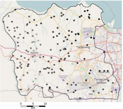
The study area was the Tengarang region to the west of Jakarta in Indonesia (Fig. 1).
203
MODIS surface reflectance from the MOD09A1 product was selected for analysis,
204
dated from 16th March 2012. This product provides a modified version of the
205
ground-level atmospheric scattering or absorption computed from MODIS level 1B
206
product (Vermote et al., 2011). It is an 8-day composite with 7 bands at 464-m
207
spatial resolution. The 7 bands record surface spectral reflectance with wavelengths
208
of 620-670nm, 841-876nm, 459-479nm, 545-565nm, 1230-1250nm, 1628-1652nm
209
and 2105-2155nm. MODI“
210
J Eklundh, 2004) and only data
211
flagged as good or marginal in the MOD09A1 reliability layer were extracted from
212
the original time series data. Band 5 captures short wave infrared reflectance and is
213
sensitive to water vapour. It commonly has a few missing values due to strip noise
214
(Wang et al., 2011) and so an inverse distance weighting interpolation was used to
215
predict (or infill) them. Each MODIS band image consisted of 6200 pixel sites.
216
217
Land cover ground data at 494 randomly selected locations was collected by visual
218
interpretation of the VHR image layers in Google Earth. At each location, the
219
proportions of different land cover types were recorded for an area the size of the
220
MOD09A1 grid cell. Eight land cover types were recorded (Urban, Settlement,
largest area in each cell was used to label that cell. This ground data was then
223
associated with its corresponding imagery data.
224
225
[image:11.595.89.509.178.548.2]226
Fig. 1. the study area to the west of Jakarta, Indonesia with the 494 land cover
227
ground data, with a transparency term to show their density, and an OpenStreetMap
228
backdrop.
229
230
In order to objectively assess classification accuracy of , the
231
combined ground/imagery data were randomly divided into training and validation
232
subsets using a class-stratified 80/20 split. These 80/20 splits were repeated 100
233
times and the classification procedures applied to the 100 different splits. The
234
distribution of land cover classes for the described training/validation split is given in
235
0 5 10
Table 1. Observe that the training data set size is relatively small, and as such, will
236
237
238
Table 1. Class-stratified training/validation split for land cover ground data.
239
Urban Settlement Paddyfield Cultivated Trees Grass Bare Water
Training 26 96 190 22 11 32 15 4
Validation 6 24 47 5 3 8 4 1
240
3.2. GWPCA
241
242
For GWPCA, a localised PCA is computed at target locations, allowing a local
243
identification of any change in the structure of a multivariate data set. Formally, if
244
spatial location has coordinates , then GWPCA involves a vector of observed
245
variables being conceptualised as having a certain dependence on its location ,
246
where and are the local mean vector and the local
variance-247
covariance matrix, respectively. The local variance-covariance matrix is
248
249
, (1)
250
251
F
252
-253
254
if otherwise, (2)
255
i
u,vi
x i
u ,i vi
u ,i vi
ui,vi
XTW
ui,vi
XX n m
u ,i vi
W
2
21 d r
where the bandwidth is the geographic distance , and is the distance between
256
spatial locations of the and rows in . As with any GW model, other kernel
257
shapes are possible (Gollini et al., 2015). To find the local PCs at location , the
258
decomposition of the local variance-covariance matrix provides the local eigenvalues
259
and local eigenvectors (or loading vectors) with
260
261
, (3)
262
263
A
264
265
, (4)
266
267
I
268
269
270
271
272
T GWPCA
273
274
E
275
276
277
r dij
th
i jth X
u ,i vi
ui,vi
ui,vi
ui,vi
ui,vi
TL V
L
u ,i vi
L V
u ,i vi
u ,i vi
T
ui,vi
XL
ui,vi
T
th
i
th
i ith
u ,i vi
tr Vm m
m m mm
278
A GWPCA was used to generate spatially-varying PCAs for the image data. A GWPCA
279
loadings data set for a given image band, for a given PC, reflects a
spatially-280
distributed set of correlations between the observations of the original band and the
281
GWPCA scores for the chosen PC. GWPCA loadings provide a local summary of each
282
band's local variance together with the local covariances, and because of this they
283
succinctly encapsulate the multivariate spatial structure in the image data. This is the
284
prime reason why they are considered worthy as input variables to improve land
285
cover classification accuracy. For the case study data (and for a given GWPCA
286
bandwidth), GWPCA loadings data sets are generated, together with
287
GWPCA scores data sets. Thus a considerable amount of data is
288
generated.
289
290
Both PCA and GWPCA results are presented, where for the PCA the image bands
291
were standardised to specify the covariance matrix. The same globally standardised
292
data were also used in the GWPCA, which is similarly specified with (localised)
293
covariance matrices. As with any PCA-based study there are consequences of these
294
data pre-processing decisions and different results may occur (e.g. Eklundh and
295
Singh 1993). Furthermore, for GWPCA, data that are globally standardised does not
296
guarantee that the data will retain their associated properties at the scale of each
297
localised PCA. A detailed presentation on the consequences of these data
pre-298
processing decisions when applying (PCA and) GWPCA, together with a list of
299
pragmatic data checks, is given in Harris et al. (2015).
300
301
49 7 7
43400 7
303
In remote sensing, supervised classification proceeds by examining the
304
characteristics of the training data (image and ground data) to be used in the
305
classification and allocates image objects to classes based on their characteristics at
306
the validation sites. In this study, the image input data was supplemented with the
307
GWPCA loadings and then with the GWPCA scores of the image data itself.
308
309
Three classification algorithms were applied: (a) a latent discriminant analysis (LDA)
310
implementation of maximum likelihood, (b) a logistic regression (LR), and (c) support
311
vector machines (SVM). These were implemented using the following functions and
312
associated R packages, respectively: lda in MASS (Venables and Ripley, 2002),
313
multinom innnet (Ripley, 2013) and svm ine1071 (Meyer et al., 2012). In all cases,
314
the default arguments for the parameterisation of the classifiers were retained. For
315
details, please refer to the R package manuals.
316
317
Classification algorithms were chosen according to their common usage and the fact
318
that each classifier could be reliably run without additional manipulation or input
319
parameters. Furthermore, the LDA and LR classifiers (which are broadly similar)
320
provide a useful contrast to SVM which takes a quite different (machine learning)
321
approach to classification. This rather naïve selection of algorithms provides some
322
objectivity to this study, as it provides a focus to the performance of GWPCA-derived
323
input variables, not the classification algorithms themselves. Future work could
324
expend the choice of algorithms and more accurately assess whether a given
325
algorithm is particularly suited to GWPCA-derived input variables.
326
3.4. Bandwidth Selection for GWPCA
328
329
Bandwidth choice is of great importance to any GW approach. Small bandwidths
330
result in greater spatial variation in the local outputs and the results of using large
331
bandwidths get increasingly close to the global metric. Bandwidths can be found in
332
an adaptive form, where the number of nearest neighbours is fixed, or in a fixed
333
form, where the distance is fixed. In this study, only adaptive bandwidths were
334
specified. For a standard implementation of GWPCA, an automatic bandwidth can be
335
found using a cross-validation procedure as detailed in Harris et al. (2011; 2015). This
336
procedure optimally selects the bandwidth according to a minimised fit between the
337
raw data and the scores data.
338
339
The aim was to use GWPCA outputs as inputs to improve land cover classification
340
accuracy. As such, it made sense to find a GWPCA calibration (i.e. its bandwidth)
341
whose outputs provided the most accurate classification. Only the GWPCA loadings
342
needed to be considered in this exercise as the GWPCA scores data should be found
343
from a small, user-specified bandwidth reflecting their use for anomaly detection.
344
The bandwidth selection procedure used in this study is described as follows:
345
346
i. GWPCA
347
GWPCA
348
T
349
PCA their nearest 62 neighbours. F
350
PCA their nearest 310 neighbours,
ii. The 80/20 classification assessment (i.e. now at the 494
353
ground data sites) was repeatedly re-run using the same raw image data, but for
354
each run a different set of GWPCA loadings data was used from step (i). Here it
355
soon became apparent that GWPCA loadings data via a 20% bandwidth would
356
provide the most accurate classification results (at least on average for each
357
classifier over the 100 runs). Thus for clarity, the accuracies in Table 3 were found
358
21 times corresponding to the most accurate results.
359
360
Observe that step (ii) of this procedure is sub-optimal in that a more accurate set of
361
results would be possible if an optimal bandwidth was retained for: (a) each
362
individual training/validation data split and (b) each classifier (i.e. LDA, LR and SVM).
363
However, such level of detail would distract . It was also
364
considered useful to have a broad understanding of the spatial scale at which the
365
image-derived GWPCA loadings were best able to discriminate between land cover
366
classes. A single bandwidth allows this, where a 20% bandwidth uses the nearest
367
1240 neighbouring pixels. Thus in summary, a 20% bandwidth was user-specified but
368
was strongly guided by the given validation exercise in step (ii) above.
369
370
Also observe that the bandwidth selection procedure is potentially compromised in
371
step (i) in that any given set of ground data validation sites (always some
class-372
stratified random allocation of 98 sites from 494 sites) is always included in the
373
bandwidth selection procedure. That is, each set of GWPCA loadings data was in part
374
derived from image information at the 98 validation sites, where the extent of
375
contamination at any one of 6200 pixels accorded to its proximity to a validation site.
The question then arises - is this a serious oversight and if so, should all validation
377
data sets be entirely unseen until the final accuracy assessment?
378
379
Although, it would have been possible to remove such validation sites from step (i),
380
and still provide GWPCA loadings data at these now unobserved sites in step (ii) (see
381
the GWPCA algorithm in section 3.2) thus negating this issue altogether, a revision
382
was not undertaken for the following three reasons:
383
384
a. It would have entailed that in step (i), the GWPCA algorithm would have had to
385
run 21x100 =2100 times to reflect the 21 bandwidth choices together with the
386
100 training/validation data splits.
387
b. It was likely that each set of GWPCA loadings data would change little if the image
388
data at the 98 validation sites (1.6% of the image) were included or not. In turn,
389
the final selection of a 20% bandwidth would still be likely.
390
c. The chosen 20% bandwidth was itself a (deliberately) sub-optimal selection.
391
392
Thus in the interest of parsimony and pragmatism, such a revision was not followed.
393
All further results of this study were considered similarly unaffected by this decision.
394
395
Furthermore, this issue is only concerned with the creation of variables for input into
396
a classification algorithm. It is not concerned about the testing of the classification
397
itself, as is usually the case in a training/validation exercise and here, in step (ii),
398
the validation data still remained unseen in this sense. A final point worth noting is
399
that there would be no advantage to only focus on the 494 ground data sites (i.e.
computationally. A bandwidth found using this relatively sparse data (see Fig. 1b)
402
would not directly transfer to that which is required for the full image data.
403
404
4. Results
405
406
4.1. PCA
407
408
For any GW model application, it is informative to consider its global counterpart for
409
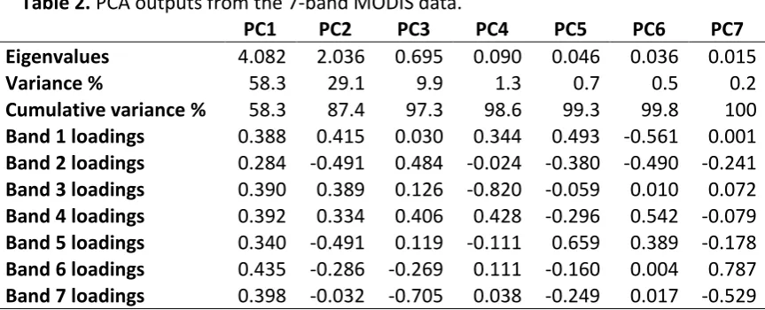
reference. The PCA results are shown in Table 2 and indicate that a subsequent
410
analysis could justifiably proceed retaining only the first (PC1) and second (PC2)
411
components as both have eigenvalues that are greater than 1 and together they
412
account for 87.4% of the total variance. This level of explained variance amongst
413
only the first two PCs reflects strong levels of collinearity amongst the MODIS bands,
414
which is not unexpected with this type of data. Interrogation of a simple correlation
415
matrix confirms this, with strong correlations (p > 0.85) between Bands 1 and 3,
416
Bands 1 and 4, Bands 2 and 5, Bands 3 and 4, Bands 5 and 6, Bands 6 and 7. The PCA
417
loadings indicate that Band 6 contributes most to PC1 and that Bands 2 and 5 equally
418
contribute the most to PC2.
419
[image:19.595.78.510.605.780.2]420
Table 2. PCA outputs from the 7-band MODIS data.
421
PC1 PC2 PC3 PC4 PC5 PC6 PC7 Eigenvalues 4.082 2.036 0.695 0.090 0.046 0.036 0.015
Variance % 58.3 29.1 9.9 1.3 0.7 0.5 0.2
Cumulative variance % 58.3 87.4 97.3 98.6 99.3 99.8 100
Band 1 loadings 0.388 0.415 0.030 0.344 0.493 -0.561 0.001
Band 2 loadings 0.284 -0.491 0.484 -0.024 -0.380 -0.490 -0.241
Band 3 loadings 0.390 0.389 0.126 -0.820 -0.059 0.010 0.072
Band 4 loadings 0.392 0.334 0.406 0.428 -0.296 0.542 -0.079
Band 5 loadings 0.340 -0.491 0.119 -0.111 0.659 0.389 -0.178
Band 6 loadings 0.435 -0.286 -0.269 0.111 -0.160 0.004 0.787
422
4.2. GWPCA
423
424
A GWPCA was then applied to the same data, generating local eigenvalues, local
425
variance proportions, local cumulative variance proportions, local loadings data sets
426
and local scores data sets, across the 6200 image sites. The GWPCA can assess how
427
the dimensionality in the imagery can vary across the study region via the local
428
variances and how the multivariate structure of the imagery can vary via the local
429
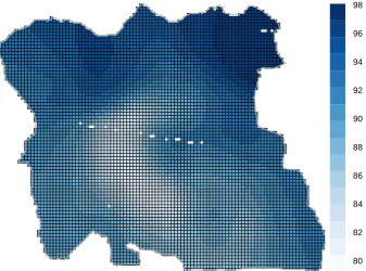
loadings data sets. Fig. 2a shows the spatial distribution of the variance proportions
430
accounted for by PC1 and how they vary geographically from the global value of
431
58.3%. Fig. 2b shows the distribution of cumulative variance proportions for PC1
432
and PC2 combined, which was 87.4% globally. It is evident that PC1 explains much
433
more of the variance in the north eastern corner of the study region (Fig. 2a), whilst
434
together PC1 and PC2 explain more of the cumulative variance in the northern and
435
eastern areas of the study region (Fig. 2b). These areas are also most likely to exhibit
436
the strongest levels of (local) collinearity amongst the image bands. Image
437
dimensionality clearly varies across the study region, where for all areas the
438
PC
439
440
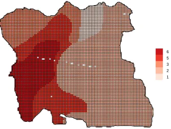
Investigating and visualising the loadings data from GWPCA is a challenge, and in this
441
respect, various visualisation tools can be found in Harris et al. (2011; 2015). The
442
difficulty lies in the fact that at every local PCA location, the loadings data for each
443
band and PC needs to be somehow viewed and related to each other. For this study,
444
a simple visualisation is adopted where the image bands with the largest (absolute)
dominate PC1 within the study region and that Band 6, which dominates globally,
447
only dominates in a north western and a north eastern area (Fig. 3a). Locally, it now
448
appears that Bands 1 and 4 contribute more to PC1, than Band 6 does. Similarly,
449
Bands 2 and 5 that contributed the most to PC2, do not dominate PC2 throughout
450
the study region (Fig. 3b). Although in this instance, Band 2 displays a degree of
451
homogeneity - as it provides the highest absolute loading for over 50% of the region.
452
453
Although this has intentionally been only a brief demonstration of GWPCA, it has
454
highlighted that both dimensionality and structure in the image data can vary across
455
the study region. In particular, as image-band structure (via the loadings) clearly
456
exhibits spatial variation then this information has the potential to act as a useful
457
discriminator of land cover, which is now assessed.
458
a)
-700000 -690000 -680000 -670000
650000 660000 670000 680000 690000
b)
Fig. 2. Spatial distribution of the local variances proportions explained by a) PC1 and
459
b) PC1 and PC2 combined, from a GWPCA. Global variance proportion for PC1 was
460
58.3%. Global cumulative variance proportion for PC1 and PC2 combined was 87.4%.
461
a)
-700000 -690000 -680000 -670000
650000 660000 670000 680000 690000
80 82 84 86 88 90 92 94 96 98
-700000 -690000 -680000 -670000
650000 660000 670000 680000 690000
b)
Fig. 3. Spatial distribution of the image bands with largest (absolute) local loadings
462
for a) PC1 and b) PC2, from a GWPCA. Corresponding global PCA results were
463
respectively Band 6, and Bands 2 and 5, jointly.
464
465
4.3. Land Cover Classification
466
467
A series of supervised classifications were undertaken with four groups of input
468
variables: (1) the seven image bands only (2) the image-derived GWPCA loadings for
469
PC1 and PC2 only, (3) the image data plus the GWPCA loadings, and (4) the image
470
data plus the GWPCA loadings plus the GWPCA ranked scores. As the global PCA
471
indicated that the first two PCs were the most important, then this was assumed to
472
be true for the GWPCA with respect to the loadings. To provide some spatial context
473
to the different input data and how they vary across the study region, Figures 4, 5
474
and 6 shows in their full form the MODIS imagery and the GWPCA image band
475
loadings for PC1 and for PC2.
476
477
-700000 -690000 -680000 -670000
650000 660000 670000 680000 690000
For input variable group 4, the GWPCA ranked scores data capture local multi-band
478
outlier information. Harris et al. (2014b) found that the most promising outlier
479
detection method resulted from observations with extreme local scores values from
480
either the first PC or from the last PC. Thus two additional texture input variables
481
were constructed to reflect the ranking of the local scores data for each of PC1 and
482
for PC7, where the lower the ranking, the more likely that the MODIS pixel is locally
483
anomalous in a multi-band (or multivariate) sense. These extra input variables
484
(simply termed GWPCA ranked scores) may help classify a land cover that is
485
somewhat obscure, or occurs in an unexpected location/setting. In this instance, the
486
GWPCA run was calibrated with a much smaller (user-specified) bandwidth of 2.5%,
487
as GWPCA was now being used to detect anomalies.
488
489
491
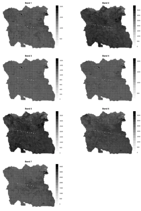
Fig. 4. Inputs into land cover classifications: the MODIS imagery
492 Band 1 −700000 −690000 −680000 −670000
650000 660000 670000 680000 690000
500 1000 1500 2000 Band 2 −700000 −690000 −680000 −670000
650000 660000 670000 680000 690000
0 500 1000 1500 2000 2500 3000 3500 Band 3 −700000 −690000 −680000 −670000
650000 660000 670000 680000 690000
0 200 400 600 800 1000 1200 1400 1600 Band 4 −700000 −690000 −680000 −670000
650000 660000 670000 680000 690000
500 1000 1500 2000 Band 5 −700000 −690000 −680000 −670000
650000 660000 670000 680000 690000
0 500 1000 1500 2000 2500 3000 3500 Band 6 −700000 −690000 −680000 −670000
650000 660000 670000 680000 690000
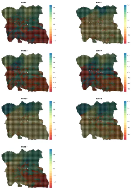
Fig. 5. Inputs into land cover classifications: the GWPCA band loadings for PC1 493 494 Band 1 −700000 −690000 −680000 −670000
650000 660000 670000 680000 690000
−0.6 −0.4 −0.2 0.0 0.2 0.4 0.6 Band 2 −700000 −690000 −680000 −670000
650000 660000 670000 680000 690000
−0.4 −0.2 0.0 0.2 0.4 0.6 Band 3 −700000 −690000 −680000 −670000
650000 660000 670000 680000 690000
−0.6 −0.4 −0.2 0.0 0.2 0.4 0.6 Band 4 −700000 −690000 −680000 −670000
650000 660000 670000 680000 690000
−0.6 −0.4 −0.2 0.0 0.2 0.4 0.6 Band 5 −700000 −690000 −680000 −670000
650000 660000 670000 680000 690000
−0.4 −0.2 0.0 0.2 0.4 0.6 Band 6 −700000 −690000 −680000 −670000
650000 660000 670000 680000 690000
−0.4 −0.2 0.0 0.2 0.4 0.6 Band 7 −700000 −690000 −680000 −670000
650000 660000 670000 680000 690000
−0.4 −0.2
Fig. 6. Inputs into land cover classifications: the GWPCA band loadings for PC2 495 496 Band 1 −700000 −690000 −680000 −670000
650000 660000 670000 680000 690000
−0.6 −0.4 −0.2 0.0 0.2 0.4 0.6 Band 2 −700000 −690000 −680000 −670000
650000 660000 670000 680000 690000
−0.8 −0.6 −0.4 −0.2 0.0 0.2 0.4 0.6 0.8 Band 3 −700000 −690000 −680000 −670000
650000 660000 670000 680000 690000
−0.6 −0.4 −0.2 0.0 0.2 0.4 0.6 Band 4 −700000 −690000 −680000 −670000
650000 660000 670000 680000 690000
−0.6 −0.4 −0.2 0.0 0.2 0.4 0.6 Band 5 −700000 −690000 −680000 −670000
650000 660000 670000 680000 690000
−0.6 −0.4 −0.2 0.0 0.2 0.4 0.6 Band 6 −700000 −690000 −680000 −670000
650000 660000 670000 680000 690000
−0.6 −0.4 −0.2 0.0 0.2 0.4 0.6 Band 7 −700000 −690000 −680000 −670000
650000 660000 670000 680000 690000
−0.4 −0.2
Following the procedures described in section 3, LDA, LR and SVM classifiers were
497
run 100 times across 494 ground data sites using class-stratified 80/20
498
training/validation data splits (see Table 1) with the four input variable groups
499
described. For each run, the overall accuracy percentage for each classifier was
500
determined from the diagonal of a standard correspondence matrix, comparing the
501
class of the validation data with the predicted class. The resultant mean overall
502
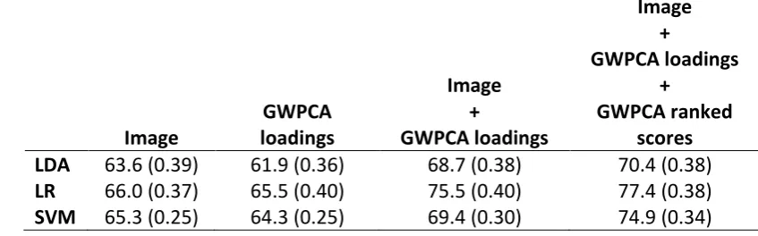
accuracies for 100 runs are presented in Table 3, indicating that classification
503
accuracy is broadly similar for each of the three classifiers when just the image data
504
are used, and also when just the GWPCA loadings are used. However when the
505
image data are combined with the GWPCA loadings, the accuracies increase
506
markedly. This suggests that including variables that describe the spatial multivariate
507
structure of the imagery improves classification predictive strength. There are only
508
slight improvements in accuracy when the GWPCA ranked scores data were included
509
as inputs. However, these marginal improvements were entirely expected given that
510
the focus was on anomalies and by definition, they should be fairly rare. On average
511
over the 100 runs, LR is consistently the most accurate classifier, in this instance.
512
[image:28.595.76.500.632.764.2]513
Table 3. The mean overall accuracy percentages for four different input variable
514
groups to a set of three different classification algorithms. Corresponding standard
515
errors of the means (SEMs) are in brackets. The number of input variables per group
516
were 7, 14, 21 and 23, respectively.
517
518
Image
GWPCA loadings
Image +
GWPCA loadings
Image +
GWPCA loadings +
GWPCA ranked scores
LDA 63.6 (0.39) 61.9 (0.36) 68.7 (0.38) 70.4 (0.38)
LR 66.0 (0.37) 65.5 (0.40) 75.5 (0.40) 77.4 (0.38)
520
To provide a fuller understanding of the results of Table 3, Table 4 describes the
521
results per land cover class. It show the improvement from using the image data only
522
(input variable group 1) to using the image data plus the GWPCA loadings plus the
523
GWPCA ranked scores (input variable group 4). These results need to be viewed in
524
context of the training/validation data splits given in Table 1, where for land cover
525
classes that are poorly represented (or rare), the classification improvement is often
526
quite marked, whereas for land cover classes that are relatively well represented
527
(Settlement and Paddyfield), classification accuracy is sometimes marginally
528
reduced. These results provide clear value in the GWPCA-based methodology to
529
accurately classify land cover across the full spectrum of possible classes, and in
530
doing so, goes someway in justifying the extra complexity that the new methodology
531
introduces into the classification procedure.
532
533
Table 4. Changes in mean overall accuracy for each land cover class, comparing the
534
I I GWPCA GWPCA
535
group.
536
Urban Settlement Paddyfield Cultivated Trees Grass Bare Water LDA 38.2 to 68.0 71.2 to 68.1 86.2 to 79.3 8.2 to 75.4 20.0 to 20.0 18.6 to 54.5 1.2 to 35.5 0 to 68 LR 42.5 to 63.5 74.0 to 78.0 88.9 to 84.8 6.6 to 80.2 19.3 to 20.7 16.6 to 59.9 1.5 to 62.5 0 to 99 SVM 1.8 to 45.5 83.4 to 82.9 92.5 to 92.8 0 to 48.6 1.3 to 13.3 7.4 to 45.5 0 to 22.8 0 to 0
537
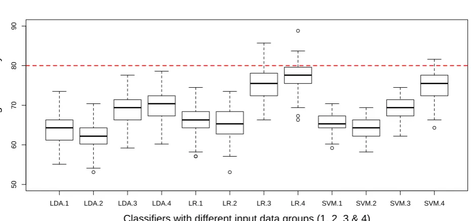
Fig.7 shows the full distributions of the accuracy results as summarised in Table 3,
538
from all 100 of the class-stratified 80/20 training/validation data splits. The boxplots
539
of the accuracy distributions clearly shows that the use of GWPCA-derived inputs
540
improves classification accuracy. The greatest improvements were found with the LR
541
classifier, where for some training/validation data splits, land cover classification
542
accuracy exceeds 80%. The boxplots also confirm that the SVM classifier consistently
543
has lower variance in the results than the LDA or LR classifiers. Paired t-tests were
used to test for significance differences in the means of selected accuracy
545
distributions and are summarised in Table 5. All of the key differences that have
546
been reported are highly significant.
547
548
[image:30.595.62.527.173.391.2]549
Fig. 7. Distributions of classification accuracy data from 100 runs of the
550
training/validation data splits. Classifiers (LDA, LR, SVM) denoted with input groups
551
(1-Image, 2-GWPCA loadings, 3-Image+GWPCA loadings, 4-Image+GWPCA
552
loadings+GWPCA ranked scores). Given with an 80% accuracy line for context.
553
554
Table 5. Paired t-test results for differences in mean overall accuracies, with input
555
groups as follows: 1-Image, 2-GWPCA loadings, 3-Image+GWPCA loadings,
4-556
Image+GWPCA loadings+GWPCA ranked scores.
557
Groups 1 vs. 2 Groups 1 vs. 3 Groups 1 vs. 4 Groups 3 vs. 4
LDA p < 0.0019 p < 0.0000 p < 0.0000 p < 0.0018
LR p < 0.2945 p < 0.0000 p < 0.0000 p < 0.0005
SVM p < 0.0083 p < 0.0000 p < 0.0000 p < 0.0000
558
559
5. Discussion
560
561
The results of Table 3 indicate that use of the MODIS image data alone (Fig. 4) or the
562
GWPCA loadings alone (Fig. 5 and 6) result in similar land cover classification
563
LDA.1 LDA.2 LDA.3 LDA.4 LR.1 LR.2 LR.3 LR.4 SVM.1 SVM.2 SVM.3 SVM.4
5
0
6
0
70
8
0
90
Classifiers with different input data groups (1, 2, 3 & 4)
P
e
rc
e
n
ta
g
e
A
c
c
u
ra
c
the GWPCA loadings as texture variables. This improvement is because the local
565
loadings arising from GWPCA capture important spatial heterogenic effects in the
566
multi-band structure of the image data via variances and covariances. This
567
information reflects spatially-distributed sets of correlations between the
568
observations of the original bands and the GWPCA scores and describes the local
569
contribution of each band to each PC. The results imply that if a loadings structure
570
were to be associated with each land cover class it would not be fixed, but instead
571
would vary geographically placing land cover in context with its locality. Further, but
572
more marginal improvements in accuracy were found when the GWPCA ranked
573
scores were included as inputs. Here only slight improvements were expected given
574
that these inputs should only help classify a land cover that is somewhat obscure, or
575
occurs in an unexpected location/setting. The results of Tables 4 and 5 and Fig. 7
576
were given to provide clarity and detail to those summarised in Table 3, providing
577
added value to the GWPCA-based land cover classification methodology.
578
579
In this study the classifications were undertaken from a standpoint of naivety. It is
580
well known that collinearity might be expected between certain image bands and
581
this was the case here. Furthermore, many of the 14 different GWPCA loadings
582
datasets are themselves highly collinear. Evidence of this can be seen in Fig. 5 and 6
583
and is not surprising given the collinearity of the image bands. Collinearity can result
584
in a loss of model precision and a loss of power in a classification model's parameter
585
estimates. There are a number of ways to reduce such global collinearities. An initial
586
step of image band selection could be applied to help identify specific types of
587
features, for example, red and infra-red bands to support biomass analyses. Also, the
588
image bands and GWPCA loadings data that are highly collinear could be removed,
the first two global PCs of the image data could be used with the GWPCA loadings, or
590
a classification technique could be specifically designed to accommodate collinear
591
variables such as a penalised or shrinkage approach (see Tibshirani, 1996). Removal
592
of collinear image bands and GWPCA loadings data and using only the first two
593
global PCs of the image data were experimented with, but found to make little
594
difference to the classification results. This was not surprising given that collinearity
595
tends to have more of an effect on model inference rather than the model's ability
596
to provide accurate predictions.
597
598
Of note however, is that of the three classifiers, SVM is itself a penalised or shrinkage
599
method in that it has a regularisation term. This may in part explain why the SVM
600
classifier consistently performed better than the LDA or LR classifiers with respect to
601
its spread of results (see Table 3 and Fig. 7). This is because the standard error of the
602
means (SEMs) are consistently smaller than that found with LDA and LR. However, as
603
only the default arguments for the optimisation of its parameters were used, the
604
SVM classifier would still require some user-input to check that the regularisation
605
term and any kernel parameters were correctly calibrated.
606
607
I
608
A
609
610
I
611
612
There is no reason why
spatial resolution or over a much larger area. Thus issues of scale should not unduly
615
compromise this new classification method. What is important to local techniques is
616
that sufficient information is available so that important spatial heterogeneities can
617
be reliably captured. Future work will
618
-619
620
Unlike many moving window or partitioned-based methods, a GW approach makes
621
much better use of available information, as it is still possible to use all the data
622
whilst still modelling local effects. For example, a 100% bandwidth of this study was
623
still able to provide localised PCAs because a distance-decay (bi-square) kernel was
624
specified. Similarly, much attention in GW modelling is placed in finding optimal
625
kernel bandwidths so that the scale at which each localised model operates is
626
appropriately determined. Future work will compare similarly localised classification
627
methods to the one demonstrated here, providing further context to the
GWPCA-628
based method.
629
630
I GWPCA
631
H GWPCA
632
GWPCA could be applied for an
633
optimisation of the image data collection, or the detection of image band outliers
634
(e.g. Harris et al., 2014a; b). I
635
636
This study adds to a growing body of work that has used
637
GWPCA to provide a greater understanding on how dimensionality and structure in
638
multivariate data can vary spatially including research in the social sciences
(Fotheringham et al., 2002; Lloyd, 2010, Harris et al., 2011) and the environmental
640
sciences (Kumar et al., 2012; Harris et al., 2015).
641
642
T
643
H GWPCA
-644
645
- T GW
646
GW
647
T
648
-
649
H
650
GW Páez
651
652
GWPCA T
653
654
655
I
656
-
657
658
659
6. Conclusions
660
661
This research has found that the
662
GWPCA GWPCA
665
-666
I
667
668
669
Acknowledgements
670
The authors would like to thank Prof Heiko Balzter and the Centre for Landscape and
671
Climate Research at the University of Leicester, and the JSPS program International
672
network-hub for future earth: research for global sustainability for supporting this
673
research. Research is also supported by the Biotechnology and Biological Sciences
674
Research Council of the UK (BBSRC BB/J004308/1). All of the statistical analysis and
675
mapping were implemented in R version 3.2.0, the open source statistical software
676
(http://cran.r-project.org). The code and data used in this analysis will be provided
677
to interested researchers on request.The authors would like to thank the
678
anonymous reviewers whose comments helped significantly improve this article.
679
680
References
681
Abdel-Aziz, Y. I., & Karara, H. M. (2015). Direct Linear Transformation from
682
Comparator Coordinates into Object Space Coordinates in Close-Range
683
Photogrammetry. Photogrammetric Engineering & Remote Sensing, 81(2),
103-684
107.
685
Atkinson, P.M., & Lewis, P. (2000) Geostatistical classification for remote sensing: an
686
introduction. Computers & Geosciences 26, 361-371
Atkinson, P.M. (2004) Spatially weighted supervised classification for remote
688
sensing. International Journal of Applied Earth Observation and
689
Geoinformation 5(4), 277-291.
690
Atkinson, P.M., & Naser. D.K. (2010) A Geostatistically Weighted k NN Classifier for
691
Remotely Sensed Imagery. Geographical Analysis 42(2), 204-225.
692
Belkin, M., & Niyogi, P. (2003). Laplacian eigenmaps for dimensionality reduction and
693
data representation. Neural Computation, 15(6), 1373-1396.
694
Brunsdon, C., Fotheringham, A.S. & Charlton, M.E.(2002) Geographically weighted
695
summary statistics - a framework for localised exploratory data analysis.
696
Computers, Environment and Urban Systems, 26, 501-524.
697
Brunsdon, C., Fotheringham, A.S. & Charlton, M. (2007), Geographically Weighted
698
Discriminant Analysis, Geographical Analysis, 39, 376-396.
699
Brunsdon, C., Fotheringham, A.S. & Charlton, M. (1996), Geographically Weighted
700
Regression: A Method for Exploring Spatial Nonstationarity. Geographical
701
Analysis, 28(4), 281-298.
702
Campbell, J., (1981). Spatial correlation effects upon accuracy of supervised
703
classification of land cover. Photogrammetric Engineering of Remote Sensing,
704
47, pp. 355 364.
705
Car, J.R., & Miranda, F.P. (1998) The semivariogram in comparison to the
co-706
occurrence matrix for classification of image texture. IEEE Transactions on
707
Geoscience and Remote Sensing 36(6), 1945-1952
708
Chica-Olmo, M. & Abarca-Hernandez, F. (2000). Computing geostatistical image
709
texture for remotely sensed data classification. Computers & Geosciences,
710
26(4), 373-383.
Collins, J. B. & Woodcock, C. E. (1996). An assessment of several linear change
712
detection techniques for mapping forest mortality using multitemporal Landsat
713
TM data. Remote Sensing of Environment, 56(1), 66-77.
714
Comber A.J., (2013). Geographically weighted methods for estimating local surfaces
715
of overall, user and producer accuracies. Remote Sensing Letters, 4(4):
373-716
380.
717
Comber, A., Fisher, P.F., Brunsdon, C. & Khmag, A. (2012). Spatial analysis of remote
718
sensing image classification accuracy. Remote Sensing of Environment, 127:
719
237 246
720
Congalton, R. G., (1988). Using spatial auto-correlation analysis to explore the errors
721
in maps generated from remotely sensed data. Photogrammetric Engineering
722
and Remote Sensing, 54, 587-592.
723
Congalton, R. G. (1991). Remote Sensing and Geographic Information System Data
724
Integration: Error Sources and. Photogrammetric Engineering & Remote
725
Sensing, 57(6), 677-687.
726
D U H , P., Brunsdon, C., Fotheringham, A.S., & McLoone, S. (2013).
727
Principal components analysis on spatial data: an overview. Annals of the
728
Association of American Geographers 103, 106 128.
729
Deng, J.S. Wang, K. Deng, Y.H. & Qi, G.J. (2008). PCA-based land-use change
730
detection and analysis using multitemporal and multisensor satellite data.
731
International Journal of Remote Sensing,29, 4823 4838.
732
Doxani, G., Karantzalos, K., & Tsakiri-Strati, M. (2011). Monitoring urban changes
733
based on scale-space filtering and object-oriented classification. International
734
Journal of Applied Earth Observation and Geoinformation, 15, 38 48.
Eklundh, L., & Singh, A. (1993). A comparative analysis of standardised and
736
unstandardised principal components analysis in remote sensing. International
737
Journal of Remote Sensing, 14(7), 1359-1370.
738
Filzmoser, P., R. Garrett, & Reimann, C. (2005). Multivariate Outlier Detection in
739
Exploration Geo-chemistry. Computers & Geosciences,31, 579 87.
740
Filzmoser, P., R. Maronna, & Werner, M. (2008). Outlier Identification in High
741
Dimensions. Computational Statistics and Data Analysis 52, 1694 711.
742
Foody, G.M. (2005) Local characterization of thematic classification accuracy
743
through spatially constrained confusion matrices. International Journal of
744
Remote Sensing,26, 1217-1228.
745
Fotheringham, A.S., Brunsdon, C., Charlton, M. (2002), Geographically Weighted
746
Regression the analysis of spatially varying relationships. Wiley, Chichester
747
Getis, A., Ord, J.K. (1992) The Analysis of Spatial Association by Use of Distance
748
Statistics. Geographical Analysis 24, 189-206.
749
Gollini, I., Lu, B., Charlton, M., Brunsdon, C., & Harris, P. (2015). GWmodel: an R
750
package for exploring spatial heterogeneity using geographically weighted
751
models. Journal of Statistical Software, 63.
752
Hansen, M., Dubayah, R., & DeFries, R. (1996). Classification trees: an alternative to
753
traditional land cover classifiers. International Journal of Remote Sensing,
754
17(5), 1075-1081.
755
Harris, P., Charlton, M., Fotheringham, A.S. (2010) Moving window kriging with
756
geographically weighted variograms. Stochastic Environmental Research and
757
Risk Assessment 24, 1193-1209
Harris P., Brunsdon C., Charlton M. (2011) Geographically weighted principal
759
components analysis. International Journal of Geographical Information
760
Science, 25:1717-1736.
761
Harris P., Clarke A., Juggins S., Brunsdon C., Charlton M. (2014a) Geographically
762
weighted methods and their use in network re-designs for environmental
763
monitoring. Stochastic Environmental Research and Risk Assessment, 28:
1869-764
1887.
765
Harris P., Brunsdon C., Charlton M., Juggins S., Clarke A. (2014b) Multivariate spatial
766
outlier detection using robust geographically weighted methods. Mathematical
767
Geosciences, 46(1) 1-31.
768
Harris P., Clarke A., Juggins S., Brunsdon C., Charlton M. (2015) Enhancements to a
769
geographically weighted principal components analysis in the context of an
770
application to an environmental data set. Geographical Analysis, 47: 146-172.
771
Harsanyi, J. C., & Chang, C. I. (1994). Hyperspectral image classification and
772
dimensionality reduction: an orthogonal subspace projection approach.
773
Geoscience and Remote Sensing, IEEE Transactions on, 32(4), 779-785.
774
Hubert, M., P. J. Rousseeuw, & K. Vanden Branden, (2005). ROBPCA: A New
775
Approach to Robust Principal Component Analysis. Technometrics,47, 64 79.
776
Ingebritsen, S. E., & Lyon, R. J. P. (1985). Principal components analysis of
777
multitemporal image pairs. International Journal of Remote Sensing, 6(5),
687-778
696.
779
Johnson, B., Ryutaro, T, Zhixiao, Xie. (2012) Using geographically weighted variables
780
for image classification. Remote Sensing Letters 3(6), 491-499.
781
Jönsson, P., & Eklundh, L. (2004). TIMESAT a program for analyzing time-series of
782
satellite sensor data. Computers & Geosciences, 30(8), 833 845.
Koutsias, N., Mallinis, G., & Karteris, M. (2009). A forward/backward principal
784
component analysis of Landsat-7 ETM+ data to enhance the spectral signal of
785
burnt surfaces. ISPRS Journal of Photogrammetry and Remote Sensing, 64(1),
786
37-46.
787
Kumar, S., R. Lal, & Lloyd, C. (2012). Assessing spatial variability in soil characteristics
788
with geographically weighted principal components analysis. Computational
789
Geosciences, 16, 827 835.
790
Legendre, P., & Legendre, L. (1998). Numerical Ecology, 2nd ed. Amsterdam: Elsevier.
791
Lloyd, C. D. (2010). Analysing population characteristics using geographically
792
weighted principal components analysis: a case study of Northern Ireland in
793
2001. Computers, Environment and Urban Systems, 34(5), 389-399.
794
Meyer, D., Dimitriadou, E., Hornik, K., Weingessel, A., & Leisch, F. (2012). e1071:
795
Misc Functions of the Department of Statistics (e1071), TU Wien, 2012. R
796
package version, 1-6.
797
Myint, S. W. (2003). Fractal approaches in texture analysis and classification of
798
remotely sensed data: Comparisons with spatial autocorrelation techniques
799
and simple descriptive statistics. International Journal of Remote Sensing,
800
24(9), 1925-1947.
801
Páez, A., Farber, S., Wheeler, D. (2011) A simulation-based study of geographically
802
weighted regression as a method for investigating spatially varying
803
relationships, Environment and Planning A 43(12), 2992-3010.
804
Pesaresi M. & J. A. Benediktsson, (2001). A new approach for the morphological
805
segmentation of high-resolution satellite imagery. IEEE Transactions on
806
Geoscience and Remote Sensing, 39, 309 320.
Pohl C. & Van Genderen J.L., (1998). Multisensor image fusion in remote sensing:
808
Concepts, methods and applications. International Journal of Remote Sensing,
809
19(5), 823-854.
810
Propastin, P. (2012). Modifying geographically weighted regression for estimating
811
aboveground biomass in tropical rainforests by multispectral remote sensing
812
data. International Journal of Applied Earth Observation and Geoinformation,
813
18, 82-90.
814
Pugh, S.A. & R.G. Congalton (2001). Applying spatial autocorrelation analysis to
815
evaluate error in New England forest-cover-type maps derived from Landsat
816
Thematic Mapper data. Photogrammetric Engineering and Remote Sensing
817
67(5), 613-620.
818
Richards, J.A. (1984). Thematic mapping from multitemporal image data using the
819
principal components transformation. Remote Sensing of Environment,
16:35-820
46.
821
Riemann, R., Wilson, B. T., Lister, A., & Parks, S. (2010). An effective assessment
822
protocol for continuous geospatial datasets of forest characteristics using USFS
823
Forest Inventory and Analysis (FIA) data. Remote Sensing of Environment,114,
824
2337-2352.
825
Ripley, B. (2013). Feed-forward neural networks and multinomial log-linear
826
URL http://www. stats. ox. ac.
827
uk/pub/MASS4.
828
Soille P (2003). Morphological Image Analysis: Principles and Applications, Springer,
829
New York, NY, USA, 2nd edition.