Structured Mesh Generation : Open-source automatic nonuniform mesh generation for FDTD simulation

nonuniform mesh generation for FDTD simulation. White Rose Research Online URL for this paper: http://eprints.whiterose.ac.uk/100155/

Version: Accepted Version

Article:

Berens, Michael, Flintoft, Ian David orcid.org/0000-0003-3153-8447 and Dawson, John Frederick orcid.org/0000-0003-4537-9977 (2016) Structured Mesh Generation :

Open-source automatic nonuniform mesh generation for FDTD simulation. IEEE Antennas and Propagation Magazine. pp. 45-55. ISSN 1045-9243

https://doi.org/10.1109/MAP.2016.2541606

[email protected] https://eprints.whiterose.ac.uk/ Reuse

Items deposited in White Rose Research Online are protected by copyright, with all rights reserved unless indicated otherwise. They may be downloaded and/or printed for private study, or other acts as permitted by national copyright laws. The publisher or other rights holders may allow further reproduction and re-use of the full text version. This is indicated by the licence information on the White Rose Research Online record for the item.

Takedown

If you consider content in White Rose Research Online to be in breach of UK law, please notify us by

1

Open Source Automatic Non-uniform Mesh

Generation for FDTD Simulation

Michael K. Berens, Ian D. Flintoft,

Senior Member, IEEE,

and

John F. Dawson,

Member, IEEE,

Abstract—This article describes a cuboid structured mesh generator suitable for 3D numerical modelling using

techniques such as finite-difference time-domain (FDTD) and transmission-line matrix (TLM). The mesh generator takes as its input an unstructured triangular surface mesh such as is available from many CAD systems, determines a suitable variable mesh discretisation and generates solid and surface meshes in a format suitable for import by the numerical solver. The mesher is implemented in the MATLAB language and is available as open source software.

Index Terms—mesh generation, ray-casting, finite-difference time-domain, transmission-line matrix

F

1

I

The finite-difference time-domain (FDTD) method is a numerical technique that is widely used to solve Maxwell’s differential equa-tions in the time domain [1]. Both space and time are discretised. Space is discretised into rectangular-shaped elements in 2D or cuboid elements in 3D. Cuboid elements, where the electric fields are located on the edges of the cuboid and the magnetic fields normal to the faces, are called Yee-cells and are the funda-mental elements of most FDTD methods [2]. By filling up the problem space with these cells, we obtain a 3D mesh, where neighbouring cells share edges and faces. Each cell has three associated electric and magnetic field compo-nents, while the other field components be-long to adjacent cells. The properties of each cell are adjusted to represent materials such as dielectrics or conductors by adjusting the constitutive parameters used in the field equa-tions in the corresponding cells, hence forming

• J. F. Dawson, and I. D. Flintoft are with the Department of

Electronics, University of York, York YO10 5DD, U.K. (e-mail [email protected], [email protected]).

• M. Berens is with the Institut f ¨ur Grundlagen der

Elektrotech-nik und MeßtechElektrotech-nik, University of Hanover, Hanover D-30060, Germany.

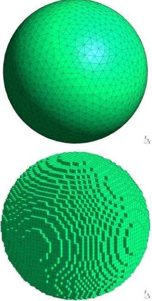
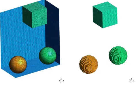
the geometrical structure of the problem to be solved. For example, Figure 1 shows a sphere and a version of the sphere discretised using cubic elements.

Algorithms for automatic structured mesh generation have been developed since the ca-pabilities of the FDTD method and computer hardware reached the point at which relatively complex geometries could be simulated. A se-lection of the techniques proposed are reported in [3], [4], [5], [6], [7], [8], [9], [10], [11]. The process of generating a cuboid structured mesh from an arbitrary model geometry consists of two main steps. The first is to determine an efficient placement of the structured mesh lines, constrained by the numerical requirements of the FDTD method, to “best fit” the model ge-ometry and the second is the identification of which structured mesh cell belongs to which object, a process called material mapping.

solution for many problems is found. Another local approach was proposed in [13], where the numerical error, caused by a rapid change of mesh size, is reduced by considering only the two cells on either side of a transition point between two intervals. There are also global approaches with a focus on all the in-tervals of a mesh [14]. Less constrained Carte-sian mesh generation algorithms have also been developed, e.g. for the Conformal FDTD al-gorithm [15], [16], [17] and for the hybrid FDTD/FETD algorithm [18]. Another indepen-dent category of non-uniform mesh generation is adaptive mesh refinement (AMR) [19], [20], [21]. This method is used to refine the mesh in regions of interest after (or during) a simulation without creating a completely new mesh.

A number of different ray tracing methods have been reported for the material mapping stage. A good method should be fast, memory conserving and capable of handling different kinds of special cases, e.g. intersections in a very narrow angle or exactly in the object plane, edge or node. These special cases can cause “singularities” and make the ray casting more difficult to implement. These issues are explained in more detail in [22] and [23]. Very efficient ray casting approachs are described in [24] and [25].

Although there are many freely available computer-aided design (CAD) or meshing pro-grams that can directly create an unstructured polygonal mesh there are no freely available meshers that create structured cuboid meshes with sufficient generality for practical EM sim-ulations of complex structures. Therefore we have developed a MATLAB [27] code for uni-form and non-uniuni-form structured mesh gener-ation and published it as open source software. The code also works in GNU Octave [28]. The output data format has been kept quite generic so it can be easily adapted to create structured output meshes for a wide range of numerical solvers. While the mesher is mostly based on the known algorithms briefly reviewed above, we hope the open-source nature of the code will make it useful to research and teaching institutions that write and use their own nu-merical solvers. Moreover, the code can be used

Fig. 1. Unstructured triangular mesh (top) and structured cubic mesh (bottom) of a sphere.

as a tool to aid the understanding of mesh generation, and for experimentation with mesh generation techniques.

The geometry of structures to be modelled using an FDTD solver must be defined by some means which allows the production of a suitable cuboid mesh. Here we assume the description is principally in the form of an unstructured triangulated mesh describing the surface of each object, such as that shown in the top part of Figure 1 for a sphere, since such a representation can be generated by most CAD software packages.

2

S

FOR

FDTD

in such a way that the geometrical structure can be represented appropriately and the numerical error is acceptably small. However the smaller the cell size the larger the memory consumed and the longer the run-time for a given prob-lem. Therefore a mesher should produce mesh lines with the largest spacing that satisfies the above constraints.

2.1 Numerical errors due to cell size and cell size variation

Numerical errors are inherent undesired ef-fects within the classical Yee-cell based FDTD-methods that originate from numerical disper-sion and anisotropy. In other words they orig-inate from the dependence of the numerical wave propagation velocity in the mesh on fre-quency and direction [29]. Because numerical dispersion causes cumulative phase errors and non-physical refraction, it is necessary to min-imize these effects. In general the dispersion error per wavelength can be expressed as

ψerr = 2π· λ e λ −1

!

, (1)

where λ/λe is the ratio of the exact (continu-ous space) wavelength to the numerical wave-length. The more cells there are per wavelength, the closer the numerical wavelength is to the exact one. Since the Yee-cell based FDTD algo-rithm is second-order accurate, the dispersion error decreases by a factor m2

if the cell size decreases by a factor m. The effect of disper-sion can therefore be reduced to an acceptable level by setting the mesh size appropriately. The typical “rule of thumb” is that the mesh size should be at most dmax ≤ λ/10 with the

mesh spacing in each direction,dx, dy, dz ≤dmax

[30]. For many problems a finer mesher with

dmax ≤ λ/20 or dmax ≤ λ/30 may be necessary

to achieve the required accuracy.

The central-difference formulation used in many FDTD codes is only accurate to first-order locally if the mesh in non-uniform, though it re-mains accurate to second-order globally [31]. In the interests of accuracy it is therefore better to keep the mesh as uniform as possible and limit the mesh size ratio between neighbouring cells

to a number close to unity. Nevertheless there are advantages of non-uniform meshes, which allow a fine mesh where geometrical detail or field variation requires (for example material interfaces) and a coarse mesh elsewhere. This allows a trade-off between numerical error and computational efficiency. In addition, a variable mesh cell size allows the mesh-to-object fitting to be adjusted, which can be important, for ex-ample, to ensure accurate resonant frequencies are obtained. Nevertheless, the ratio of adjacent mesh cell sizes needs to be constrained; in most cases it is sufficient to chose the upper limit for this ratio asdi/di+1 <1.5.

3

A

MESH GENERATION

3.1 Input unstructured mesh

Since most CAD packages are capable of ex-porting an unstructured mesh, regardless of their internal representation, we chose to use an unstructured mesh, rather than a particular CAD representation as input to the mesher. For the internal unstructured and structured mesh formats we created a format based on those defined in the AMELET-HDF specification [34]. These formats are quite general and allow the definition of mesh nodes and various mesh ele-ments like line eleele-ments (two nodes) and trian-gles (three nodes). The AMELET-HDF formats, which were specifically developed for com-putational electromagnetics applications, also allow naming groups of elements of different types like nodes, lines, surfaces in order to iden-tify these types of object in the mesh and allow the allocation of different material properties to each group.

Fig. 2. Flow chart of a typical work-flow for generating the input unstructured mesh.

between a CAD program and the mesh genera-tor introduced in this article. Figure 2 illustrates a typical work-flow using a CAD tool such as FreeCAD to generate the original geometry which can be saved in a suitable intermediate format forGmsh.

3.2 Generating a uniform structured mesh

As mentioned above, a uniform mesh min-imises the magnitude of certain numerical er-rors and therefore it is the basic mesh for FDTD simulations. It is also simpler to implement and understand than a mesh where the cell size varies, but still provides a good introduction to some of the issues of structured mesh genera-tion.

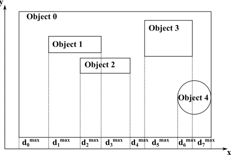
Consider a problem scenario where objects with different electromagnetic properties are present such as in Figure 3. In our mesher, the maximum mesh size, dmax, is constrained such

that the mesh cells are less than or equal toλ/10

in the material with the shortest wavelength (this is can be defined manually or determined from a material database using the frequency dependent constitutive parameters of the mate-rial). A minimum mesh size, dmin, is specified

Object 0

Object 1

Object 2

Object 3

Object 4 y

x d0max _d1max _d2max _d3max _d4max_d5max _d6max_d7max

Fig. 3. Example of overlapping objects in one coordinate direc-tion (x_).

manually. In order to fit the geometry to the mesh, the mesher must choose a mesh size be-tween these limits which best fits the geometry of the objects to be meshed. The maximum uniform mesh size is bounded above by the smallest mesh size of all the intervals,

dmax = min(dmaxi ≤λ/10), (2)

whereiindexes the intervals. Whendmin =dmax

the algorithm simply uses the defined mesh size without any optimization.

We take a simple approach to a best fit by trying to find a mesh size in each coordinate direction that ensures that the edge of each object’s bounding box lies on a mesh line. We define the edge of each object’s axis aligned bounding box (AABB) in each dimension as a constraint point which divides the mesh into a number of intervalsdias shown in Figure 3. The

constraint points (i.e. interval boundaries) are defined by Xi (i = 1, . . . , Nx),Yi (i = 1, . . . , Ny)

and Zi (i= 1, . . . , Nz), where Nx,Ny,Nz are the

number of constraints in the respective direc-tions. These points have to be part of the mesh to guarantee the mesh is adjacent to the objects. Since the restriction dmin prevents this

The uniform mesh lines are defined by

xi =X1 +i·dx,opt i= 0, ..., nx−1 yi =Y1+j·dy,opt j = 0, ..., ny−1, zi =Z1+k·dz,opt k = 0, ..., nz−1

(3)

wheredi,optis the unknown optimum mesh size

in the i-direction and nx, ny and nz are the

number of mesh lines in the specified direction. The next step aims to satisfy the condition that all the constraint points are closely aligned with a mesh line by independently minimizing the functions

fx(dx,opt) = NXx−1

i=1

∆Xi dx,opt

!

fy(dy,opt) = N_Xy−1

j=1

∆Yj dy,opt

!

fz(dz,opt) = NXz−1

k=1

∆Zk dz,opt

!

(4)

with

∆Xi =Xi+1−Xi i= 1, ..., Nx−1 ∆Yj =Yj+1−Yj j = 1, ..., Ny −1, ∆Zk =Zk+1−Zk k = 1, ..., Nz−1

(5)

using the golden section search with parabolic interpolation algorithm available inMATLAB’s

fminbnd function. In the case of several equal solutions, the one with the largest value of

dopt is chosen to minimize the computational

time. If a cubic mesh is required then the sum

fx(dopt) + fy(dopt) + fz(dopt) is minimised in a

single optimisation.

After dopt is known it is still necessary to

determine the optimum offset of the mesh lines relative to the constraint points. Therefore we carry out another optimisation to simultane-ously minimize the functions

gx(x0) =

Nx

X

i=1

|Xi−x0−x|

gy(y0) =

Ny

X

j=1

|Yi −y0−y|,

gz(z0) =

Nz

X

k=1

|Zi−z0−z |

(6)

where x,y and z are the mesh lines calculated using (3) and (4) and x0, y0 and z0 are the

Fig. 4. Example of a uniform mesh solution for three overlapping objects.

offsets to be determined. For this MATLAB’s multi-variable gradient-based fmincon optimi-sation function is used. Because the solution of (6) is periodic, the offsets are limited to the ranges defined by0≤x0 ≤dx,opt,0≤y0 ≤dy,opt

and 0 ≤ z0 ≤ dz,opt. Since this step shifts the

origin of the mesh, it is necessary to extend the mesh in order to ensure that it still encloses the objects to be meshed. The position of the mesh lines are therefore

x=X1−x0+i·Dx,opt i= 0, ..., nx y =Y1−y0+j·Dy,opt j = 0, ..., ny. z =Z1−z0+k·Dz,opt k = 0, ..., nz

(7)

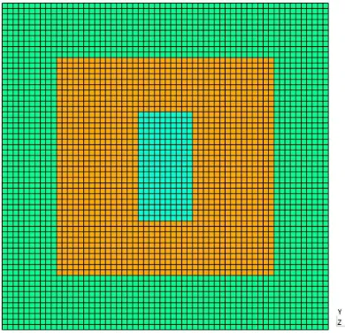
A practical example of the results of the algorithm can be seen in Figure 4, where a uniform mesh has been generated to represent three overlapping objects by using the smallest mesh size defined by one of the objects. The structured mesh shown is the optimal mesh solution found by the above algorithm, with all object boundaries aligned with the mesh lines. The full implementation also allows weights to be assigned to different constraints so the user can control the optimisation process.

3.3 Generating a non-uniform mesh

most mesh scenarios is a much more com-plex problem. Each object may impose different mesh size limits, objects may overlap on any axis and the rate of change of mesh size is lim-ited; all these interactions must be considered to produce a good mesh. For simplicity we present the treatment of only one axis in the following -the process is identical for each axis. This means that the aspect ratio of the cells is not currently constrained directly, though the way that the maximum mesh size in each material is used in the constraints in each direction indirectly limits the ability of the algorithm to generate high aspect ratio cells.

Considering a scenario similar to the one in Figure 3, it is first necessary to create a 1D projection of the objects on to each axis. For each interval delineated by the object bound-ing boxes, the object with the smallest defined maximum mesh size, dmax

i , must dominate all

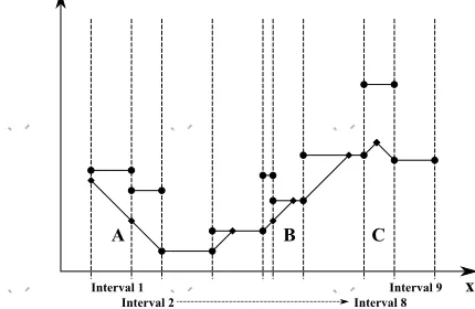
other overlapping objects when the mesh is generated. If we take the maximum mesh size for each interval, as determined from the object with the smallest maximum mesh size in that interval, and plot it against position on one axis a plot like that of Figure 5 is obtained.

In order to produce a viable mesh we must honour the maximum mesh size in each inter-val. However in order to minimise the number of mesh elements we must allow the mesh size to grow when we progress from an interval with a small maximum mesh size to an interval with a larger mesh size. The growth in mesh size being limited by the maximum cell size ratio rmax. Figure 6 shows the possible growth

in mesh size from each interval added to the interval mesh sizes of Figure 5. We now know for all interval boundaries the maximum mesh size that can be created, either by the respective interval itself or by growth of the mesh size from neighbouring intervals.

Figure 7 shows the next step. In order to avoid exceeding rmax, the smallest mesh size

has to be selected at each boundary. If this mesh size was determined by mesh growth from a smaller cell it is continued until it either ends in another subinterval boundary (position A) or until it exceeds the maximum mesh size,

dmax

i , of the current subinterval (position B) as

x

Interval 1

Interval 2 Interval 8 Interval 9

dx_imax

Fig. 5. The maximum allowed mesh size in each interval along thex_-axis.

x d_ximax

Interval 1

Interval 2 Interval 8

Interval 9

Fig. 6. Geometric progression of mesh sizes from each interval.

x d_ximax

Interval 1

Interval 2 Interval 8 Interval 9

A B C

Fig. 7. Initial selection of smallest mesh size at interval bound-aries and extension of growth lines.

x d_ximax

Interval 1

Interval 2 Interval 8 Interval 9

A B C

d_{iA d}

iB

L L_M

L_A L_B

d_i

x d_imax

Fig. 9. Mesh size for interval for a non-uniform mesh that grows from both sides reaching the interval maximumdmax

i .

d_{iA d}

iB L

LA LB

di

x dimax

1/2(L - LB+ LA)

Fig. 10. Mesh size for interval for a non-uniform mesh that grows from both sides and does not reaching the interval maximum

dmax_{i before clashing.}

illustrated in Figure 7. Another possible mesh solution occur if two geometric progressions intersect before oversteppingdmax

i (position C).

Now we can choose the line of smallest mesh size in each interval as shown in Figure 8. Having now determined the feasible limit of mesh size in each interval we have to place the mesh lines. However it should be pointed out that Figure 8 represents only an approximate solution as there must be an integer number of mesh cells in each interval if the interval bound-aries are to be maintained. Mesh lines, which satisfy the mesh size and ratio constraints, can be created locally for each interval with the information for each interval illustrated in Fig-ure 8.

There are a number of scenarios that can occur in each interval and each must be treated individually. Figure 9 shows the mesh size dx

across an interval of lengthLfor the case where the mesh size grows and reaches its maximum value, dmax

i , within the interval. LA is the

dis-tance from the left boundary over which the mesh size grows, LM is the distance for which

the mesh size remains constant at its maximum value, and LB is the distance over which the

mesh grows from the right boundary. LA and LBare initially not known. The number of mesh

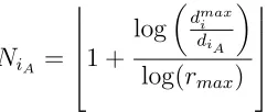
cells,NiA, in LAis

NiA =

     1 +

log dmax i d_iA

log(rmax)

      (8)

where⌊z⌋ is the largest integer smaller than or equal to z and diA is the mesh size at the left

boundary. Now, as NiA is rounded down to an

integer we have a maximum mesh size less than

dmax

i afterNiA mesh cells, which is sufficient to

meet the mesh size criterion, that is

rNmaxiAdxA ≤d max

i . (9)

The length of the transition region,LA, can now

be computed by summing the geometric series

LA= N_iA

X

i=1

diAr N_iA max=diA

1−rNmaxiA

1−rmax

. (10)

Similarly forLB

NiB =

     1 +

log dmax i d_iB

log(rmax)

      (11) and

LB =diB

1−rNiB

max

1−rmax

. (12)

It should be clear that after the preprocessing resulting in a solution similar to the example in Figure 8 there is no scenario withdiA > d

max i or diB > d

max i .

IfLA+LB < L, then the situation is as shown

in Figure 9, with LM = L − LA − LB. Now LM might not correspond to an exact number

of cells of size dmax

i that will respect the ratio

between the intersection points of LA, LM and LB. If necessary we must modify the number

of cells and cell ratios in LA and LB by

incre-menting NiA and NiB and reducing the step in

cell sizes to reduce LM to an exact number of

uniform cells (possibly zero). This is achieved by an iterative solution.

If LA +LB > L then the situation is as in

Figure 10. Here we must compute the point at which the cell sizes intersect with 1/2 · (L −

LB + LA) and modify NiA, NiB and the step

Fig. 11. Example of a non-uniform mesh showing a slice through three different regions and the generated mesh lines.

Fig. 12. Input unstructured mesh (left) and generated structured mesh (right) of three objects.

the ratio condition. This is also achieved by an iterative solution.

A practical 2D example of the results of the algorithm can be seen in Figure 11, where a non-uniform mesh is used to represent three overlapping objects. The mesh size increases from the smallest to the largest ensuring that the electromagnetic properties of the objects are respected as well as the object boundaries.

4

A

-PING

4.1 Ray casting

After the positions of the mesh lines are cal-culated, it is necessary to identify which

struc-tured mesh cells or faces belong to which mesh objects in the input unstructured mesh so that the correct material properties can be assigned. This process is called material mapping. In this paper the ray casting method is considered. In essence, a set of rays are cast through the computational domain and the intersections of the rays with the objects in the unstructured mesh are located. A fast ray-triangle intersec-tion algorithm reported [26] and implemented by [39] was used to find the intersections. This set of intersections is then projected onto the structured mesh to locate the object. While rather simple in concept the method is difficult to implement reliably due to the occurrences of “singularities” associated with borderline cases. These are discussed in more detailed below.

The directions in which the rays are cast has a significant impact on the number of singularities that occur. Casting divergent rays from a point outside the computational do-main (along a diagonal of its bounding box) is one effective strategy to minimize the effect of singularities [22]. However, for the MATLAB implementation considered here this hinders the vectorization of the algorithm. We therefore also considered an approach where the rays are cast along a line of structured cells. This allows one dimension of the ray-casting to be com-pletely vectorized using the ray-triangle inter-section algorithm implementation in [39]. The result of the mapping for a simple geometry consisting of a two cubes and a sphere is shown in Figure 12.

hierarchy. The AABB of all the triangles in each sub-volume is determined as the sub-division proceeds and stored in a binary tree structure. Now when casting a ray through the object we first test if the highest level sub-volume AABB (the whole object) intersects the ray. If it does, we descend the two branches of the tree and test for intersection of the ray with the sub-volume AABBs of the children. If there is no intersection with a child AABB then that child, and all its children, can immediately be elimi-nated from the search, potentially saving a very large number of intersections tests. If the child AABB also intersects then its children’s sub-volumes are are checked and so on down the tree. BVHs implemented in low-level languages often subdivide the object until there is only one triangle in the sub-volume. Because we are using a vectorized intersection algorithm in a high-level language there is an optimum depth for the BVH that was determined empirically to be when there are about 1000 triangles in a sub-volume. The partitioning algorithm used to divide the triangles into sub-volumes also im-pacts on the performance of the algorithm; it is best to try and balance the number of triangles in each child at the same level of the tree. In the mesher reported here we implemented a number of partitioning methods including the Surface Area Heuristic (SAH) [41].

4.2 Mesh generator for structured solid ob-jects

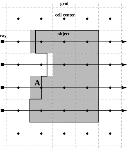
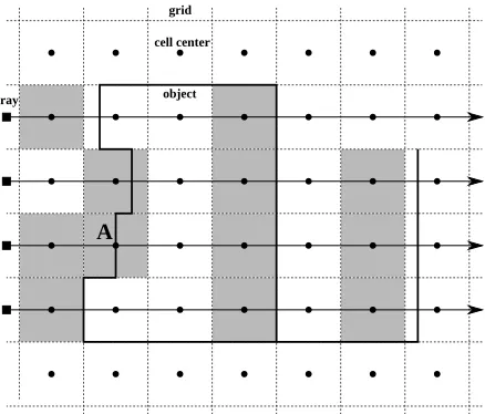
A solid is represented in the structured mesh by the volumetric material cells of the inside volume of a closed unstructured surface in the input mesh. Because both solid and surface objects are represented by a surface input mesh, it is necessary to distinguish amongst these using control parameters for each group of input objects. Thus, the input mesh for a solid is required to be a closed surface with a well defined inside which can be identified by the occurrence of an even number of intersections between ray and object. This means that it is possible to identify where a ray enters and leaves the object as shown in Figure 13. The decision about whether a cell belongs to the

grid

cell center

ray

A

object

Fig. 13. Detection of active cells when mapping solid objects.

solid structure is the main task. By selecting all cell centres between the intersection points the inside volume of the object can be identified (see the grey cells).

grid

cell center

ray

A

object

Fig. 14. Detection of active cells when mapping surface objects.

approach for the open source mesher.

Providing all the triangles in the unstruc-tured mesh have a consistent normal direction and the input mesh satisfies certain tolerances regarding triangle size it is possible to identify edge/node singularities reliably since they will be manifested as multiple intersections with triangles at the same position (within a toler-ance) along the ray, with a mixture of inward and outward facing normals. By default such intersections are regarded as non-traversing, i.e. the ray does not cross the boundary of the object. This, together with a verification that an even number of intersections are made by all the rays passing through the object ensures the global integrity of the mapping. Optionally, for improved local fidelity, a six-point interpolation based resolver can be invoked after all the object has been mapped to determine whether non-traversing singularities that occurs at a cell centers should be inside or outside the object based on the cells immediately adjacent to the singular cells [22]. A fall-back procedure that allows rays to be cast from multiple directions and the decision for each cell to be determined by a “vote” between the results for each di-rection (with user defined dictator, majority or consensus decision threshold) has also been im-plemented, though this substantially increases the computational effort.

The entire mapping algorithm depends on quite a number of interacting tolerances that

require careful tuning in order to prevent mesh-ing artifacts appearmesh-ing. Some of the tolerances are determined by an analysis of the scale and variability of the triangles in the input mesh. They can also be overidden by the user on an object-by-object basis. There is also a presumption that the input unstructured mesh does not contain any pathological features such a dramatic changes in scale comparable with the defined tolerances. Such difficulties can be avoided by applying appropriate mesh clean-ing algorithms to the input unstructured mesh before it is mapped.

4.3 Mesh generator for structured surface objects

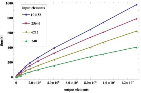
Fig. 15. Performance of the mesher with different numbers of input and output elements.

5

P

PERFORMANCE

By investigating the meshing process, we see that the number of unstructured input elements and structured output elements both have a significant influence on the performance. For clarification the number of output elements in-cludes both the cells for the both the objects themselves and the free space in the compu-tational volume. Since the mesh line generation is not significantly influenced by the number of input elements, only the material mapping is investigated in the following using a 64-bit Linux PC with an Intel Xeon E5-2687Wv2 CPU running at 3.40 GHz.

Figure 15 shows how the CPU-time in-creases with the number of output elements. Analysing models with different numbers of input elements from 240 to 101 158, a significant influence on the CPU-time can also be seen. Since the mesh line creation typically takes mil-liseconds to process, its influence on the overall runtime is negligible. The maximum analysed runtime was approximately 15 minutes for a structure with 101 158 input and 13 481 272 out-put elements.

The run-time is strongly influenced by the vectorisation of the MATLAB code and the bounding volume hierarchy. Currently the par-allelisation of the algorithm with regard to cast-ing different rays on separate computational cores has not been fully implemented. This is

Fig. 16. A wideband hybrid antenna [36].

relatively straightforward to do and will sub-stantially improve the performance on large models.

As an example of the current practical mesher performance, Figure 16 shows a wide-band hybrid antenna [36] which required a computational runtime of less than one minute (input: 12 678 elements, output: 47 360 cells). This example also demonstrates the mesher’s ability to deal with structures consisting of dif-ferent object types. The antenna model consists of a metal surface ground plane (green) and vertical metal “blade” (yellow), a solid dielec-tric pillar (blue) and a metal feed structure (red). The mesher output is a good represen-tation of the input mesh without any irregular-ities or geometric deviations.

sur-Fig. 17. Input unstructured mesh (top) and generated structured mesh (bottom) of an aeroplane [37].

face structure need longer computational run-times, e.g. the aeroplane shown in Figure 17 took 67 minutes (input: 44 847 elements, output: 503 941 914 cells). This is a complex object for the mesher since it has uneven planes at dif-ferent angles as well as holes and cuts in the surface. This surface structure can, if not rep-resented accurately, cause an incorrect electro-magnetic behaviour of the object. The mesher again achieves good conformity between the unstructured and generated structured meshes.

Another complex-shaped object can be seen in Figure 18. This object took approximately 100 minutes to map (input: 179 146 elements, output: 324 242 703 elements). Besides the com-plicated surface structure, different parts of this model overlap each other in the x, y and z

directions. If the mesher did not identify enter-ing and exitenter-ing locations of this model exactly, the structured output mesh would not conform with the unstructured mesh.

6

C

This article presents an open-source implemen-tation of an algorithm for uniform and non-uniform cuboid mesh generation for FDTD solvers and similar codes. The mesher takes an unstructured mesh as input, thus allowing great flexibility in the CAD tools that can be utilised in the initial creation of the simulation geometry.

The algorithm is based on an optimisation approach to the placement of mesh lines and the well-known ray-casting approach to mate-rial mapping. While the mesher currently does not have all the features of a commercial tool it can mesh structures of modest size with reason-able complexity, as shown by the examples pre-sented. Further work is continuing to improve the material mapping performance and feature set.

The code is available under a GPL Ver-sion 3 licence from https://bitbucket.org/ uoyaeg/aegmesher/overview.

R

[1] A. Taflove and S. C. Hagness,Computational Electromagnet-ics: The Finite-Difference Time-Domain Method, 3rd Edition, Artech House, 2005

[2] K. S. Kunz and R. J. Luebbers, The finite difference time domain method for electromagnetics, Boca Raton, CRC press, 1993

[3] W. Sun, C. A. Balanis, M. P. Purchine and G. C. Barber, Three-dimensional automatic FDTD mesh generation on a PC,Antennas and Propagation, IEEE International Symposium on, Ann Arbor, MI, pp. 30-33, 28 Jun.-2 Jul., 1993.

[4] M. Yang and Y. Chen, AutoMesh: An automatically ad-justable, non-uniform, orthogonal FDTD mesh generator, IEEE Antennas and Propagation Magazine, vol. 41, no. 2, pp. 13-19, April 1999.

[5] Y. Kanai and K. Sato, Automatic mesh generation for 3D electromagnetic field analysis by FDTD method,Magnetics, IEEE Transactions on, vol. 34, no. 5, pp. 3383-3386, Septem-ber 1998.

[6] Y. Srisukh, J. Nehrbrass, F. L. Teixeira, J.-F. Lee and R. Lee, An approach for automatic grid generation in three-dimensional FDTD simulations of complex geometries, IEEE Antennas and Propagation Magazine, vol. 44, no.4, pp. 75-80, August 2002.

[7] Y. Srisukh, J. Nehrbuss, F. L. Teixeira. JLF. Lee, and R. Lee, Automatic grid generation of complex geometries for 3-D FDTD simulations,Antennas and Propagation, IEEE Interna-tional Symposium on, Columbus, OH, pp. 326-329, 22-27 Jun., 2003.

[8] T. Ishida, S. Takahashi and K. Nakahashi, Efficient and ro-bust Cartesian mesh generation for building-cube method, Journal of Computational Science and Technology, vol. 2, no. 4, pp. 435-437, 2008.

[9] J. T. MacGillivray, Trillion cell CAD-based cartesian mesh generator for the finite-difference time-domain method on a single-processor 4-GB workstation, Antennas and Propa-gation, IEEE Transactions on, vol. 56, no. 8, pp. 2187-2190, August 2008.

[10] S. Wang and J. H. Duyn, Three-dimensional automatic mesh generation for hybrid electromagnetic simulations, IEEE Antennas and Propagation Magazine, vol. 51, no. 2, pp. 71-85, April 2009.

[11] H.-S. Kim, I. Ihm and K. Choi, Generation of non-uniform meshes for finite-difference time-domain simulations, Jour-nal of Electrical Engineering and Technology, vol. 6, no. 1, pp. 128-132, 2011.

[12] H. M. L. A. Fernanades, Development of Software for An-tenna Analysis and Design using FDTD, Portugal: University of Lisboa, 2007

[13] Y. Kanai and K. Sato, ”Automatic mesh generation for 3D electromagnetic field analysis by FD-TD method”,IEEE Transactions on Magnetics, no. 5, pp. 3383-3386, 1998 [14] H.-S. Kim, I. Ihm and K. Choi, ”Generation of

Non-uniform Meshes for Finite-Difference Time-Domain Simu-lations”,Journal of Electrical Engineering & Technology, 2011 [15] W. Yu, R. Mittra, ”A conformal FDTD software package

modeling antennas and microstrip circuit components”, IEEE Antennas and Propagation Magazine, vol. 42, no. 5, pp. 28-39, 2000

[16] Z. Su, Y. Liu, W. Yu, R. Mittra, ”A conformal mesh-generating technique for the conformal finite-difference time-domain (CFDTD) method”,IEEE Antennas and Prop-agation Magazine, vol. 46, no. 1, pp. 37-49, 2004

[17] G. Waldschmidt, A. Taflove, ”Three-dimensional CAD-based mesh Generator for the Dey-Mittra conformal FDTD algorithm”,Antennas and Propagation, IEEE Transactions on, vol. 52, no. 7, pp. 1658-1664, 2004

[18] S. Wang, J.H. Duyn, ”Three-dimensional automatic mesh generation for hybrid electromagnetic simulations”, IEEE Antennas and Propagation Magazine, vol. 51, no. 2, pp. 71-85, 2009

[19] M. J. Aftosmis, M. J. Berger and J. E. Melton, Adaptive Cartesian Mesh Generation, CRC handbook of mesh gener-ation (Contributed Chapter), 1998

[20] T. Ishida, S. Takahashi and K. Nakahashi, Efficient and Robust Cartesian Mesh Generation for Building-Cube Method, Journal of Electrical Engineering & Technology, no. 4, pp. 435-446, 2008

[21] Y. Liu, C.D. Sarris, ”AMR-FDTD: a dynamically adap-tive mesh refinement scheme for the finite-difference time-domain technique”,Antennas and Propagation Society Inter-national Symposium, vol. 1A, pp. 134-137, 2005

[22] J. Hill,Efficient Implementation of Mesh Generation and FDTD Simulation of Electromagnetic Fields, England: University of Worcester, 1996

[23] Y. E. Kalay, ”Determining the spatial containment of a point in general polyhedra”,Journal of Computer Graphics and Image Processing, no. 4, pp. 303-334, 1982

[24] S. Thon, G. Gesquiere and R.Raffin,A Low Cost Antialiased Space Filled Voxelization Of Polygonal Objects, GraphiCon ’04 Proceedings, pp. 71-78, 2004

[25] M. Szucki and J. Suchy,A Voxelization Based Mesh Genera-tion Algorithm for Numerical Models used in Foundry Engineer-ing, Journal of Metallurgy and Foundry EngineerEngineer-ing, no. 1, 2012

[27] MathWorks, MATLAB R2015a, Available: http: //de.mathworks.com/, Online, 2015

[28] Octave community,GNU Octave 3.8.1, Available: www.gnu. org/software/octave, Online, 2014

[29] J. S. Juntunen and T. D. Tsiboukis, ”Reduction of nu-merical dispersion in FDTD method through artificial anisotropy”, IEEE Transactions on Microwave Theory and Techniques, vol. 48, no. 4, pp. 582-588, 2000

[30] K. L. Shlager and J. B. Schneider, ”Comparison of the Dispersion Properties of Several Low-Dispersion Finite-Difference Time-Domain Algorithms”,IEEE Transactions on Antennas and Propagation, vol. 51, no. 3, pp. 642-653, 2003 [31] H. Jiang and H. Arai, ”Fast and efficient FDTD analysis

using non-uniform mesh for small antenna”,IEEE Antennas and Propagation Society International Symposium, vol. 2, pp. 1242-1245, 1998

[32] S. J. Owen, A Survey of Unstructured Mesh Generation Technology, IMR, 1998

[33] C. Geuzaine and J.-F. Remacle, ”Gmsh: a three-dimensional finite element mesh generator with built-in pre- and post-processing facilities”,International Journal for Numerical Methods in Engineering 79(11), pp. 1309-1331, 2009 [34] C. Giraudon,Amelet-HDF Documentation, Axessim, 2011 [35] M. Hazewinkel,Encyclopaedia of mathematics, Supplement

Volume II, Springer, 2000

[36] A. C. Marvin, G. Esposito, J. F. Dawson, I. D. Flintoft, L. Dawson, J. K. A. Everard, G. C. R. Melia, ”A wide-band hybrid antenna for use in reverberation chambers”, IEEE International Symposium on Electromagnetic Compatibil-ity (EMC), pp. 222-226, 2013

[37] 3dvia, Available: http://www.3dvia.com/content/ 2C7A92223406182A, Online, 2010

[38] 3dvia, Available: http://www.3dvia.com/content/ E3B1C7D9EBFDCFE1, Online, 2007

[39] J. Tuszynski, “Fast vectorized triangle/ray intersection algorithm”, 29 Sep. 2011. http: //uk.mathworks.com/matlabcentral/fileexchange/ 33073-triangle-ray-intersection

[40] I. Wald, S. Boulos and P. Shirley, “Ray Tracing Deformable Scenes using Dynamic Bounding Volume Hierarchies”, ACM Transactions on Graphics 26, 1, 2007.