A touch-screen controlled 'Linear Predictive Synthesizer' for accessibility applications

(1)

University of Southern Queensland

Faculty of Engineering and Surveying

A touch-screen controlled “Linear

Predictive Synthesizer” for

accessibility applications

A dissertation submitted by

Mr. Benjamin W. D. Jordan

in fulfilment of the requirements of

Courses ENG4111 and ENG4112 Research Project

towards the degree of

Bachelor of Engineering (Computer Systems Engineering)

(2)

Abstract

Numerous voice compression methods are available today for communications over low bandwidth channels. Worthy of note in particular are Linear Predictive Coding (LPC), Mixed Excitation LPC (MELP), and Code Excited LPC (CELP). The channel in these coding schemes is typically a digital transmission line or radio link, such as in cellular telephone communications, but may be other media such as files on a computer hard disk.

Linear Predictive Coding is explored in some detail as a basis for creating a new speech synthesizer that does not convert text to speech (TTS), but rather uses a touch-screen Thin Film Transistor (TFT) panel as user input to create and control voice-like audio sound synthesis.

Research has been carried out to conceptually try different methods for mapping TFT touch panel input (or any 2-dimensional input) to LPC synthesis coefficient vectors for artificial speech reproduction.

To achieve this, various LPC coefficient quantization algorithms have been explored and evaluated using Octave v.3 scripts, resulting in selection and comparison in the final hardware and software implementation.

(3)

University of Southern Queensland

Faculty of Engineering and Surveying

ENG4111/2 Research Project

Limitations of Use

The Council of the University of Southern Queensland, its Faculty of Engineering and Surveying, and the staff of the University of Southern Queensland, do not accept any responsibility for the truth, accuracy or completeness of material contained within or associated with this dissertation.

Persons using all or any part of this material do so at their own risk, and not at the risk of the Council of the University of Southern Queensland, its Faculty of Engineering and Surveying or the staff of the University of Southern Queensland. This dissertation reports an educational exercise and has no purpose or validity beyond this exercise. The sole purpose of the course pair entitled “Research Project” is to contribute to the overall education within the student's chosen degree program. This document, the associated hardware, software, drawings, and other material set out in the associated appendices should not be used for any other purpose: if they are so used, it is entirely at the risk of the user.

Prof F Bullen Dean

(4)

Certification

I certify that the ideas, designs and experimental work, results, analyses and conclusions set out in this dissertation are entirely my own effort, except where otherwise indicated and acknowledged.

I further certify that the work is original and has not been previously submitted for assessment in any other course or institution, except where specifically stated.

Benjamin W. D. Jordan

Student Number: 0031210722

Signature

(5)

Acknowledgments

“The preparations of the heart belong to man, But the answer of the tongue is from the LORD... Commit your works to the LORD, and your thoughts will be established.” (Prov. 16:1,3 NKJV)

First and foremost, regardless of the outcomes of any work undertaken I must express my deepest gratitude to God almighty because in spite of my shortcomings, bad habits and weaknesses, He has consistently shown his faithfulness in helping me overcome these barriers.

I would like to extend thanks to all the staff at the University of Southern Queensland, but in particular my project supervisor Mr. Mark Phythian and Assoc. Prof. Dr. John Leis for their help and exceptional care of the pedagogy of Electronics, Computing and Signal Processing.

Due thanks must go to my employer, Altium Limited, for providing me access to corporate resources (including hardware and software) used to implement the designs. I would like to specifically thank my manager Matthew Schwaiger for allowing me to be flexible with work commitments from time to time, and my colleague Dr. Marty Hauff for his encouragement and prayers.

Finally, it is most important to acknowledge the overwhelming love and support extended to me by my wife Erin, and our children Delta, Seth and the new addition Shiloh – born only weeks before submission.

BENJAMIN JORDAN

(6)

Table of Figures

Figure 1 Block Diagram of a Formant-based speech synthesizer ... 7

Figure 2 MELP uses formant modeling with mixed sources. ... 8

Figure 3 Formant Spaces of Australian, British and American Accents. (IEEE Signal Processing Magazine, Vol. 26 No. 3 p72, May 2009) ... 9

Figure 4 Human Speech Organs (Fu Jen Catholic University Graduate Institute of Linguistics 2007, The biological basis of speech production (2): The Vocal Tract and Related Speech Organs, viewed 22 October 2009, <http://www.ling.fju.edu.tw/phonetic/mouth.gif>). ... 12

Figure 5 Spectrogram of the voiced sound “iya”. ... 14

Figure 6 Linear Prediction FIR Filter... 19

Figure 7 All-Pole Inverse Prediction Filter ... 21

Figure 8 LPC Analysis Predictor Error and Log Magnitude Spectrum of predictor polynomial. ... 23

Figure 9 Discrete Time waveforms of input and synthesized speech frame... 24

Figure 10 Mapping a TFT Panel to Vowels and Pitch (Altium Ltd. 2009, NB2 TFT Panel Port Plug-In Library Component). ... 28

Figure 11 Z-plane Poles of a series of LPC frames from /œ/ to /U/. Blue poles mark the LPC coefficient poles of the start frame, red poles are from the final frame, and black in-between. ... 30

(14)

TABLE of Figures xiv

Figure 13 Roots of the Line Spectrum Pairs from /œ/ to /U/. ... 34

Figure 14 Line Spectrum Frequency Interpolation Using Neighbouring Angles ... 39

Figure 15 Interpolating Line Spectrum Frequencies over N frames ... 39

Figure 16 Root Expansion Algorithm ... 40

Figure 17 LPC Poles of Interpolation of coefficients using LSPs. ... 41

Figure 18 Log Magnitude Spectrum of LSP Interpolated LPC coefficients. ... 42

Figure 19 Log Magnitude Spectrum of LSP interpolations across TFT panel width. ... 43

Figure 20 Spectrogram bitmap of interpolation results used as TFT background. ... 44

Figure 21 The Software Platform Builder ... 50

Figure 22. The NB3000 running the speech synthesizer. ... 55

Figure 23 Embedded Project Memory Configuration. ... 59

Figure 24 Devices View in Altium Designer Software. This is where the FPGA and Embedded projects are downloaded to the target device. ... 61

Figure 25 Top Level FPGA Project Schematic... 99

Figure 26 FPGA OpenBus Block Diagram ... 100

(15)

Acronyms

LPC Linear Predictive Coding – a method of analysing speech based on linear

prediction, and then using the parameters obtained to synthesize it again.

CELP Code Excited LPC. MELP Mixed-Excitation LPC.

LSP Line Spectrum Pairs – a method of representing LPC parameters using

Palindromic and Antipalindromic polynomials

LSF Line Spectrum Frequencies – the angle of the roots of the LSPs

CODEC EnCOder DECoder – an audio Analogue to Digital converter and

Digital-to-Analogue converter in the same package.

I2S Inter-IC Sound bus – a multiplexed serial interface for streaming audio

A-to-D and A-to-D-to-A data.

SPI Serial Peripheral Interconnect bus – a serial interface used to connect

peripherals to host microcontrollers.

DMA Direct Memory Acces – used by the TFT panel to gain access to the pixel

display buffer.

TFT Thin-Film-Transistor (display/panel). The display used in this project is a 320

pixel wide by 240 pixel high panel, 2.4” from corner to coner diagonally.

RISC Reduced Instruction Set Computer – the CPU used in this design is a RISC

(16)

Chapter 1.

Introduction

Various speech generation systems are currently available as assistive technology. The majority are simply text-to-speech devices or software, such as the JAWS™, or simple direct speech graphical tablet style devices, such as the Static Display Speech Generators available from LifeTec Queensland.

A few problems with the current products and the approach they employ are:

 They are limited to specific language sounds (i.e. for English, French or German etc.).

 Static Display Speech Generators are limited to a pre-defined set of basic phrases.

 They do not allow for individual vocal creativity, emotions, or accents.

 They cater broadly to visually impaired, and mobility limited users, but are not particularly useful for people with a temporary speech loss.

1.1.

Objectives

(17)

1.2 Speech Synthesis Concepts 2  Create an assistive device that offers an alternative means of translating the

user’s motor movement to audible speech.

 Develop an input method that allows more generic and abstract sound generation.

 Research the feasibility of touch-screens as the input in terms of ease of use, and flexibility.

 Assess the device’s adaptability for multiple languages.

1.2.

Speech Synthesis Concepts

The advancement of speech synthesis technology has been largely driven by the need to store or transmit voice data on noisy or low-bandwidth media. Applications have ranged from long range telecommunications to children’s toys and text-to-speech devices. On the input to any good speech compression system is the analysis of the desired speech. A multitude of methods have been developed and more continue to be developed based on demand for higher quality sound intelligibility and reproduction, as well as improved human – machine user interfaces. The following are perhaps the most pervasively used methods and will be explored in some detail within this dissertation.

1.3.

Linear Predictive Coding

(18)

1.4 FPGA System on Chip Implementation 3 An LCD touch-panel and associated drivers will be used with an FPGA-based microprocessor SoC (System on Chip). This system will contain user interface software as well as the audio synthesis and filtering required for creating the desired sounds. User commands interpreted from the touch screen will control pulse and noise sources in software, which will be fed in turn through time-varying digital filters. This will be output on the system’s built-in speakers.

1.4.

FPGA System on Chip Implementation

The idea for a touch-screen controlled synthesizer initially came about when an FPGA development platform, the Altium Nanoboard-2, was being reviewed. This thought lead naturally into the concept of the assistive device for this project. Since the project commencement, Altium Limited has developed a new FPGA development platform called the Nanoboard 3000. Since then, the author has had considerable design experience through tutorial, video and reference design production to support its release to the electronics design industry. The Nanoboard 3000 has all the necessary peripherals for the touch screen synthesizer and therefore is a natural and sensible choice for prototyping the final design.

1.5.

Dissertation Structure

This dissertation is structured in the following manner:

Chapter 2 discusses the background information researched in the project, covering

(19)

1.5 Dissertation Structure 4

Chapter 3 discusses the analysis of speech by practical means. The problem of

modelling transient speech is introduced.

Chapter 4 covers voice coding mechanisms in more detail. Specifically, it delves

deeper into the topic of Linear Predictive Coding. This is then extended to discussion of how the LPC synthesis filter and source signals can be used as part of an assistive device such as the one developed.

Chapter 5 explores concepts researched for mapping voiced sounds to a

touch-screen (or any 2-dimensional) device, and the problems faced relating to time-varying the speech filter.

Chapter 6 illuminates the practical implementation of the speech synthesizer.

Infinite Impulse Response filter theory is discussed in light of the project regarding embedded systems, fixed point arithmetic, and hardware acceleration.

Chapter 7 introduces the Altium Nanoboard-3000 Xilinx Edition FPGA

development board, used in the final design. The Altium Designer software used to develop the FPGA hardware and embedded firmware for the design is also discussed, along with the actual design itself.

Chapter 8 documents the brief research undertaken into how useable the designed

speech synthesizer is, and considers the ability of the system to reproduce languages other than English.

Chapter 9 concludes the project with a brief summary of what was discovered, what

(20)

Chapter 2.

Literature Review

2.1.

Introduction

According to Cole et. al. (1996) there are essentially three classes of speech synthesizer: Articulatory, Formant-based, and Concatenative. However, work has been done since then to develop Hidden Markov Model (HMM) based synthesis by Tokuda et. al. (2000) as well – an adaptation of the concatenative approach.

Articulatory synthesis seeks to mechanically or electronically model the specific movements of the speech organs. While this could potentially provide the most accurate sounding speech, the complexity of the system is somewhat prohibitive for design and use alike.

(21)

2.1 Introduction 6 The third class, concatenative synthesizers, requires a vast library of recorded speech segments (phonemes) which are essentially strung together to form words and sentences.

Much work has been done in the past to create mechanisms for synthesizing speech, yet the majority of effort appears to have been placed on finding appropriate ways to encode speech for compact storage or transmission over narrow bandwidth channels, or for text-to-speech (TTS) systems for the visually impaired (Breen, 1992) . In terms of assistive devices, it is apparent that little effort has been directed towards those that purely generate speech from the user’s motion or command input. One very early contraption of note however, was the VODER (‘Voice Operating DEmonstratoR’) created by Homer Dudley in 1939 (Breen, 1992). The VODER used a noise source, pulse relaxation oscillator and 10 band-pass filters (Synthopia, 2009). While this was an entirely analogue design, it formed the general structure of synthesis used today in many speech coders such as the well-known LPC10 (Linear Predictive Coder, 10 Band).

Arguably, the most elegant approach of the three presented above is the formant-based synthesizer. This is due to the fact that it provides enough flexibility to produce many language sounds within reasonable limits of computing power available today.

(22)

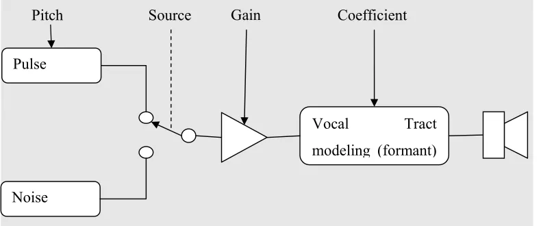
2.2 Linear Predictive Coding (LPC) 7 frequency domain of these formants have a profound effect, enabling creation of vowels in various languages. See the block diagram in Figure 1.

2.2.

Linear Predictive Coding (LPC)

In the Linear Predictive Coding speech coder, speech is sampled in wavelets and analysed for vocal tract resonance (short-term autocorrelation is used for this) and pitch (long-term autocorrelation or FFT is used for this). This information is packetized and transmitted over the channel to the synthesizer at the receiving end, as in Figure 1. Leis (unpub) has highlighted the fact that the binary choice between the pulse and noise sources as inputs limits the capability of this synthesis method and the languages it can support. For example, the sound /zh/ as in the French bon jour is not truly realizable in LPC coding, because you would need both the noise and pulse sources mixed together.

Pulse

Noise

Vocal Tract modeling (formant)

Gain Coefficient

[image:22.612.132.527.235.400.2]

Source Pitch

(23)

2.3 Mixed-Excitation LPC (MELP) 8

2.3.

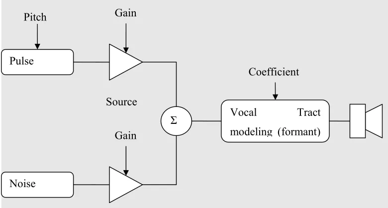
Mixed-Excitation LPC (MELP)

The MELP vocoder, an extension of the LPC vocoder, uses both noise and pulse sources at the same time, mixing them according to the parameters from the analysis (transmission). This makes for a more flexible approach that is better for synthesis of multiple languages, and provides more natural sounds during transitions in speech (ASPi, 1996). While MELP is far more computationally complex on the encoder end, it is not very much more complicated that LPC on the decoder end.

2.4.

Considerations of Language and Accent

The desire is to produce a synthesizer that could be extended to be able to facilitate any human language. This would possibly imply the use of various code books as in CELP (Code Excited Linear Prediction). Codes for source signal generation would be assembled into books that are each suitable for a specific language, say, and could be interchanged to adapt the synthesizer to different languages. The code book may

Pulse

Noise

Vocal Tract modeling (formant)

Gain

Coefficient Source

Pitch

[image:23.612.132.522.139.348.2]

Σ Gain

(24)

2.4 Considerations of Language and Accent 9 also provide a mapping from a 2-dimensional control surface such as the LCD touch screen to the generated sounds – time permitting this concept will be explored.

[image:24.612.135.450.391.639.2]

Vaseghi, Yan & Ghorshi (2009) have recently devised methods for analysing speech accents (in particular, British, American and Australian English), and morphing encoded speech from one accent to another using a Linear Prediction Formant Transformation. In this system, accent databases are used to train HMMs of speech formants for each accent. The HMMs are then used to determine the matching formant set in the target accent, and pitch intonation is also varied. The interesting thing about this work is that in analysing the different accents they developed a formant space showing another 2-dimensional view of speech parameters, shown in Figure 3. This work also highlighted the importance of pitch over time for emphasis and intonation – indicating that pitch control is essential for a good speech synthesis engine.

(25)

2.5 Parameter Quantisation and Interpolation 10

2.5.

Parameter Quantisation and Interpolation

Speech Parameters (LPC Coefficients, Gain, Error Residual and Pitch Period) can be represented in a number of ways, and various methods seek to quantise them to provide good compression without losing intelligibility.

Kabal and Ramachandran (1986) have presented a way of representing LPC coefficient vectors as Line Spectrum Frequencies the cosine angle of Line Spectrum Pairs (LSFs and LSPs). These can be quantised in terms of their angles and Paliwal (1993) has highlighted their power in this regard.

LSPs and LSFs can be utilized also for interpolating between frames of speech where a set of coefficients may have been lost due to data corruption.

(26)

Chapter 3.

Speech Analysis and Modelling

3.1.

Human Speech Organs

(27)

[image:27.612.135.414.90.355.2]

3.1 Human Speech Organs 12

Figure 4 Human Speech Organs (Fu Jen Catholic University Graduate Institute of Linguistics 2007, The biological basis of speech production (2): The Vocal Tract and Related Speech Organs, viewed

22 October 2009, <http://www.ling.fju.edu.tw/phonetic/mouth.gif>).

The main sound source within the system is the vocal cords, which operate much like a reed. The muscles surrounding the vocal cords pull them together tightly as the lungs blow air through them, causing a vibration. The sound and air pressure generated moves through the pharynx, mouth and nasal passage past the lips and nostrils respectively. The internal shapes of these cavities form resonant chambers that can arbitrarily change frequency response. Vowel sounds are generated in this way.

(28)

3.2 Insight Into Speech Analysis 13 In addition, air movement through the nose, past the tongue and through teeth and lips is used to create fricative or plosive sounds by restricting airflow or obstructing and releasing it, respectively, which in turn creates noise. Fricative sounds formed by the lips and teeth (such as /f/) relatively white since it occurs towards the outside of the cavities whereas those generated at the back of the tongue (such as /k/) shape the noise through the mouth cavity.

3.2.

Insight Into Speech Analysis

Normal humans are well known to hear sound pressure waves in the frequency range of 20 Hz – 20 KHz, yet our hearing is most sensitive in the midrange frequencies, peaking at around 4 KHz (Bauer and Torick 1966).

It is no surprise then to discover that the majority of the power in a speech signal is in this range, with lower amplitudes in the most sensitive hearing region of the spectrum, and higher amplitudes at the lower end of the spectrum.

A widely used tool for analysis of speech is the spectrogram (Rabiner and Schafer 1978). A spectrogram of a recording of the vowel transition “iya” (as in cornucopia)

is shown in Figure 5. The spectutils toolbox for Octave was used to generate a spectrogram from the recoding “iya.wav”. Spectutils can be downloaded from the University of Helsinki’s Music Research Laboratory (University of Helsinki, 2009).

(29)

[image:29.612.140.516.216.480.2]

3.3 Synthesis of Speech 14 English vowels. Their path in the transition to the “ah” sound is clearly visible – they move towards each other in the spectrum to straddle 1 KHz. There is still a lower frequency energy peak just below 100 Hz – this is indicative of the fundamental pitch of the vocal cords which is relatively constant.

Figure 5 Spectrogram of the voiced sound “iya”.

3.3.

Synthesis of Speech

The goal of any speech synthesizer is to be able to reproduce human-like sounds and as such must be able to;

(30)

3.4 Speech Transitions 15  Be able to change parameters dynamically (i.e. interpolate between speech

segments).

Each spoken language has its own set of sound combinations with varying degrees of uniqueness. In English, the vowel and semivowel sounds are formed using the two main resonance cavities, and can be modelled using two resonant filters for generating the associated formants. Most speech vowels are better modelled by four formants (Rabiner and Schafer, 1978). Each formant is modelled by two poles in the synthesis filter as they are typically complex and for a real filter to be realized would be conjugate pairs. More formants would be modelled by using more pole pairs in the linear prediction.

3.4.

Speech Transitions

Because of the transient nature of speech, the speech synthesis system must be able to adapt pitch, source selections, and gains and filter coefficients with each frame. Filters that adapt in such a way are generally referred to as Linear Shift-Variant (LSV) filters. Hence, speech is sampled into short buffers and treated as stationary for short bursts.

(31)

3.4.1 Frame Interpolation 16

3.4.1.

Frame Interpolation

Interpolation between frames is necessary if speech frames are encountered with gaps between them (i.e. a frame is lost due to corruption through the transmission channel). This interpolation is a big challenge, especially if it needs to be done in real-time.

Hui (1989) suggests LSV filters can use the Lagrange linear interpolation of filter coefficients, though this method can result in unstable filter kernels.

Goncharoff and Kaine-Krolak (1995) have devised a pole-shifting method whereby filter poles of the first frame are paired with poles of the last, and poles of interpolated frames in between the first and last are interpolated using a frequency-linear relationship. The pole pairing procedure is arduously complicated due to the ambiguity of the pole-pair relationships, and the problem that sometimes real poles must be interpolated with complex conjugate poles.

Ezzat et. al. (2005) present a fairly new method of interpolating frames of speech or music they refer to as ‘audio flow’. The principle behind it is to use a 2-dimensional morphing algorithm that is usually used in computer graphics, but lends itself to morphing the spectral envelope of the audio. It is a complex and computationally expensive algorithm, yet it provides exceptionally natural sounding results.

(32)

3.4.1 Frame Interpolation 17 i. Reflection Coefficient Interpolation

ii. Log Area Ratio interpolation

iii. Arc-sine Reflection Coefficient Interpolation iv. Cepstral Coefficient Interpolation

v. LSP (LSF) Interpolation

vi. Autocorrelation Coefficient Interpolation, and vii. Impulse Response Interpolation.

(33)

Chapter 4.

Voice Coding

4.1.

Introduction

As discussed in section 2.2, Linear Predictive Coding forms the backbone of all the currently popular speech compression mechanisms, including low-bitrate vocoders such as CELP, MELP, G.729 and others.

4.2.

Linear Predictive Coding

4.2.1.

Linear Predictor

The core of Linear Predictive Coding is, as the name suggests, a Linear Predictor (or, FIR filter put to prediction use):

(34)

4.2.1 Linear Predictor 19 The signal ̃ models a prediction based on previous samples, and therefore the LPC analysis attempts to find a set of predictor coefficients that minimize the error for each sample within the frame:

̃ 0 _{...( 4.2 )}

Substituting ...( 4.1 ) into ...( 4.2 ) gives:

...( 4.3 )

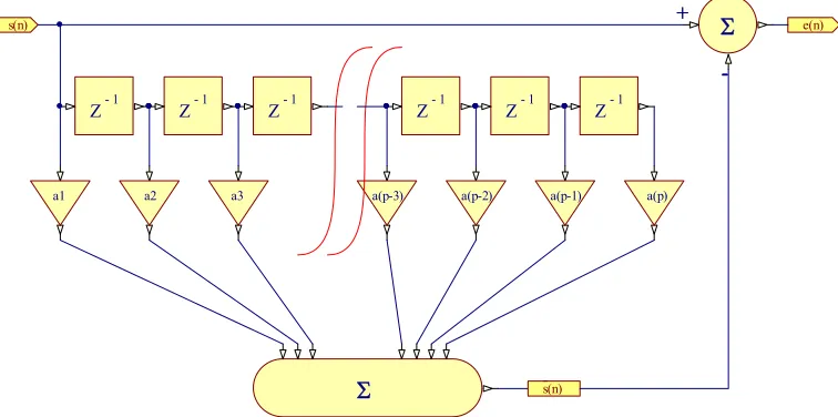
[image:34.612.139.517.452.640.2]

This is directly realizable in hardware or software as the FIR filter structure shown in Figure 6.

Figure 6 Linear Prediction FIR Filter

1

-Z

a1 a2 a3 a(p-3) a(p-2) a(p-1) 1

-Z Z-1 Z-1 Z-1 Z-1

a(p)

 s(n)

s(n) ++ e(n)

-- +

(35)

-4.2.2 Inverse Predictor 20 If the linear prediction filter was of infinite length it would allow the error residual

0 , but since any practical filter will have a finite number of taps (and any practical system could not wait forever for the result), we limit the order of prediction. The limited prediction order means that the error signal will not be zero, but instead resembles a low level noise superimposed with pulses at the fundamental frequency of the original speech frame. The limited predictor order also imposes a limit on the accuracy of the synthesis filter.

4.2.2.

Inverse Predictor

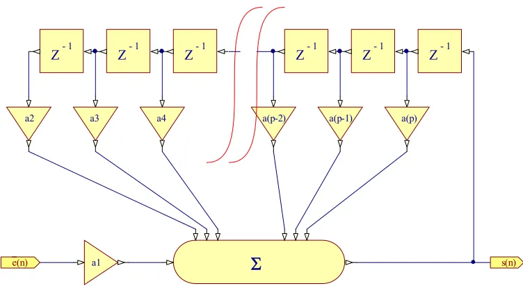
It is possible to ideally reconstruct the discrete time signal if we have the predictor coefficients and the error signal:

...( 4.4 )

(36)

[image:36.612.136.512.85.291.2]

4.2.3 Calculating Predictor Coefficients 21

Figure 7 All-Pole Inverse Prediction Filter

4.2.3.

Calculating Predictor Coefficients

The computation of predictor coefficients for a speech frame can be done using various methods including, but not limited to;

 the Covariance method,

 the Autocorrelation method, and  the Lattice method

according to Rabiner & Schafer (1978, p397).

In all of these methods, the goal is to efficiently compute the set of coefficients that minimize the mean-square error over the frame:

...( 4.5 ) 1

-Z

a1

a2 a3 a4 a(p-2) a(p-1)

1

-Z Z-1 Z-1 Z-1 Z-1

a(p)



(37)

4.2.3 Calculating Predictor Coefficients 22 Substituting ...( 4.4 ) into ...( 4.5 ) gives:

…( 4.6 )

By taking the derivative of …( 4.6 ) and setting it to zero we arrive at:

where1 …( 4.7 )

This can be solved to find the set of that minimise the error signal. This forms the basis of one of the widely implemented algorithms for LPC coefficient calculation, the Autocorrelation Method. It is computationally more efficient than other methods that were encountered during the course of this project.

Equation where 1 …( 4.7 ) can be expressed as the matrix multiplication:

, where:

1

…( 4.8 )

is the autocorrelation of the input speech frame. Equation …( 4.8 ) can be solved using an efficient algorithm known as the Levinson-Durbin Recursion (Keiler & Zölzer (ed.) 2008, p.308). Thus, the top-level algorithm for computing the predictor coefficients from a frame of speech is:

1) Input speech to BUFFER[1..N]

2) P = Predictor Order

3) R[1..P] = cross correlate ( BUFFER, P )

4) a[1..P] = Levinson-Durbin Recursion ( R, P )

(38)

[image:38.612.140.518.214.348.2] [image:38.612.139.516.217.524.2]

4.3 LPC Initial Results 23 An Octave (MATLAB) program that performs this algorithm has been provided by Keiler & Zölzer (ed.) (2008, p.308). The code listing is presented for reference in Appendix B.1.

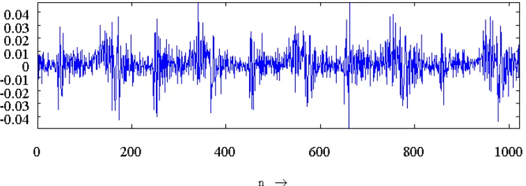
Figure 8 LPC Analysis Predictor Error and Log Magnitude Spectrum of predictor polynomial.

4.3.

LPC Initial Results

(39)

4.3 LPC Initial Results 24 (adapted from Keiler in Zölzer (ed.) (2008, p.306) performs LPC analysis on the frame taken from the named .wav file, and computes the log-magnitude FFT of the speech sample and the LPC filter overlayed. The error residual is shown above.

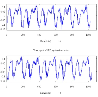
[image:39.612.138.518.313.688.2]

The lpc_gen_figs() script also generates the waveform displays in Figure 9. This provides a visual comparison of the original speech input waveform and that which is reconstructed using the error filtered through the LPC Synthesis filter (Figure 7). In this scenario the sample rate of the voice is 22.05 KHz and the prediction order chosen was 20.

(40)

4.4 LPC Parameter Quantization 25

4.4.

LPC Parameter Quantization

LPC and its variants are used for the most part in lossy communications channels, such as the GSM mobile telecommunications system, and in Voice Over IP (VOIP) network communications protocols. The underlying motivation for using vocoders like LPC is to parameterise speech so that the speech frames being transmitted are highly compressed, without perturbing the intelligibility of speech or impairing the listener’s ability to identify the speaker.

Once the LPC coefficients are calculated they form a very compact packet that is much smaller than uncompressed speech. Several approaches have been developed for quantising the speech parameters to reduce the storage or transmission load further. Worthy of particular mention in this project is the use of Line Spectrum Frequencies as discussed by Kabal & Ramachandran (1986) and Paliwal (1993).

(41)

4.5 Conclusion 26

4.5.

Conclusion

This shows that if you re-construct the encoded speech frame using the actual residual error you will achieve a close-to-ideal result. In practice the error signal is approximated (or quantized) into a pulse or white noise source, or in the case of the CELP vocoder, a code book. The code book is an array of quantized error approximations that are chosen to reconstruct the speech with minimal error.

(42)

Chapter 5.

Morphing Formants across the TFT Panel

5.1.

Introduction

The aim of this project was at first somewhat ambiguous in that it sought to map voiced and unvoiced speech sounds to a 2-dimensional control surface. The ambiguity lies in the following facts:

 It is difficult to narrow down the fundamental elements of speech to a handful of simple movements on a screen.

 Some languages produce sounds from the back of the throat and tongue that LPC does not easily reproduce.

(43)

5.2 User Interface research 28

5.2.

User Interface research

As a starting point for pragmatic research the design approach taken here is to map specific vowels to the TFT panels X-axis, while the pitch of the synthesizer is controlled by the Y-axis. The choice of using a pulsed source, noise source, or a mix of both is performed by a separate control – pushbuttons. An example of how this implementation will look is illustrated in Figure 10.

[image:43.612.135.309.430.670.2]

Phythian, M. (pers. comm.) has suggested other possibilities involving continuously adjusting the screen display to show a series or circles of symbols that depict speech sounds or code vectors. The display of these glyphs would dynamically update depending on where the pointer to the screen last was. The net result would be that the user constructs strings of phonemes and diphthongs by moving a finger or stylus around the screen. This approach is similar to a text-to-speech system except would be more generic in nature.

(44)

5.3 Morphing Across The TFT 29

5.3.

Morphing Across The TFT

With the decision made to map formants across the X-axis of the screen, the next problems that need solving are:

1. How to generate the LPC synthesis coefficients, and;

2. Once they are mapped to the screen, how to smoothly morph between them as the stylus moves.

It is also worth mentioning that the choosing and ordering of the vowels at this time is arbitrary, but research should be undertaken to gain a better understanding of how to make this choice, and would likely involve using LPC sound corpus from many languages or accents.

The first problem above is easy to solve – in this project we use recorded segments of the author’s speech, and generate the LPC coefficient vectors in non-real-time using Octave scripts.

To get an idea of what to expect in terms of Z-plane pole shifts when vowel sounds dynamically change with respect to speech frames, the Octave script ow_pole_mapping_plot.m was used to generate Figure 11. In this image, the simple phrase /œ U/ (as in ‘ouch’) was divided into 1024-sample, 50% overlapping

(45)

[image:45.612.179.430.114.395.2]

5.4 Interpolation of Coefficients 30

Figure 11 Z-plane Poles of a series of LPC frames from /œ/ to /U/. Blue poles mark the LPC coefficient poles of the start frame, red poles are from the final frame, and black in-between.

5.4.

Interpolation of Coefficients

(46)

5.5 Introducing LSPs 31 overly complex for the needs of this project. Another method, similar but simpler and easier will be used.

5.5.

Introducing LSPs

Line Spectrum Pairs, as the name suggests, are lines, paired along the spectrum (i.e., around the unit circle on the Z-plane), that describe the characteristics of the LPC filter.

They are computed in the following manner, as shown by many including Kabal and Ramachandran (1986), Soong & Juang (1993), Paliwal & Atal (1993), Stein (2002) and more.

5.5.1.

Computing the Line Spectrum Pairs

The LPC coefficient vector has the transfer function:

1 ,

where A z is the polynomial of length (i.e. LPC order) :

1 …( 5.1 )

(47)

5.5.1 Computing the Line Spectrum Pairs 32

1 1 …( 5.2 )

Similarly, an antipalindromic equation can be constructed by subtracting the mirrored coefficients:

1 1 …( 5.3 )

[image:47.612.138.358.380.603.2]

And, adding …( 5.2 ) and …( 5.3 ), P z Q z 2A z , so we sum the elements of the palindromic and antipalindromic polynomials and multiply by 0.5 to get back to the original LPC coefficient vector.

Figure 12 Roots of the Palindromic and Anti-palindromic Polynomials: LSPs

Im

Re

1

-1

(48)

5.5.1 Computing the Line Spectrum Pairs 33

P z and Q z are vectors of Line Spectrum Pairs, and have the interesting characteristic that their roots are entirely on the unit circle in the Z-plane, and the roots of P z are interleaved with those of Q z hence the term Line Spectrum Pairs. These properties are illustrated in Figure 12.

The other useful property these roots possess is that they are always complex-conjugated and if you modify their position as a conjugate pair, you will modify the formants of the LPC vector while guaranteeing a stable filter.

The Octave function lsplpc(), listed in appendix B.5 obtains the LSPs from an LPC input vector. This function first forms the palindromic and antipalindromic polynomial vectors, then uses Octave’s built-in roots() function to find their roots. The majority of papers found on LSPs are devoted to finding faster ways of computing their roots to enable their use in real-time systems. A common way is to evaluate the magnitude of the polynomials as excited by cosines of the frequencies around the unit circle and find the zero-crossing points (Kabal & Ramachandran, 1986). There is a speed versus accuracy trade-off in such computations.

(49)

[image:49.612.176.435.86.373.2]

5.6 Conclusion 34

Figure 13 Roots of the Line Spectrum Pairs from /œ/ to /U/.

5.6.

Conclusion

(50)

Chapter 6.

Practical Implementation

6.1.

Introduction

Since the overall idea is to use LPC-style vocal tract modelling for the synthesizer, it makes sense to use the now well-researched LPC synthesis mechanism along with LPC analysis.

(51)

6.2 LPC Analysis Function 36

6.2.

LPC Analysis Function

LPC analysis was performed to generate basic vowel coefficients using the Octave (or, MATLAB) script function calc_lpc() (Keiler, F & Zölzer, U (ed.) 2008, p.308). This follows the traditional method of using the Levinson-Durbin Recursion, and fortunately Octave comes equipped with the necessary function making the generation of predictor coefficients straightforward. The calc_lpc() function returns a vector of coefficients including the 1 in the denominator of the synthesis equation, as well as the gain factor for the analysed frame of speech.

Sample .wav files as discussed in Chapter 3 were recorded and clipped for the voiced sounds iii, eh, a, ah, o, ue, rr, and uw. The format of these samples was mono, 22.05 KHz sample rate and 16-bit quantization. This format provides bandwidth of 11.025 KHz (using the Nyquist theorem) and a theoretical dynamic range of greater than 90dB, which is more than adequate for speech.

(52)

6.3 LSP Calculation 37

6.3.

LSP Calculation

As discussed in Chapter 5, LSPs have been chosen as an experimental method of interpolating LPC coefficient vectors. To perform the conversion of LPC coefficients to LSPs, the function lsplpc() was developed in accordance with the algorithm presented in section 5.5.1. While most LPC vocoders would transmit only the angles of the LSPs, over one half of the unit circle (as the other is always a mirror image), this function keeps all the roots around the circle in the arrays P and Q. The angles of the LSP roots are usually referred to as Line Spectrum Frequencies (LSFs) as they are represented as angles versus complex numbers. This also reduces frame packet size. For this project, the lsplpc() function keeps the LSPs in separate vectors for convenience (Ph and Qh) though they are not strictly necessary.

6.3.1.

Roots of the Line Spectrum Pairs

The lsplpc() function also calculates the LSP roots and returns them as a vector with complex numbers. Because the LSP roots lie around the unit circle, they can be expressed as pure angles (LSFs). LSFs are calculated using:

…( 6.1 )

And conversely, converted back into complex representation with:

(53)

6.3.2 Interpolation Using LSFs 38 One important point here is that, because LSFs are mirrored on the bottom-half Z-plane, when converting from LSFs back to LSPs it is necessary to also subtract the imaginary sine term.

In this project the conversion back to LSPs from LSFs is done in the interpolation function, described in the next sub-section.

6.3.2.

Interpolation Using LSFs

Interpolation of LSFs is as simple as linear interpolation of angles. Figure 14 illustrates this process. The two frames to be interpolated and the number of interpolation steps are given to calculate angle step size:

∆ ….( 6.3 )

(54)

[image:54.612.133.320.83.277.2]

6.3.2 Interpolation Using LSFs 39

Figure 14 Line Spectrum Frequency Interpolation Using Neighbouring Angles

Figure 15 Interpolating Line Spectrum Frequencies over N frames

[image:54.612.134.435.354.591.2]

(55)

6.3.3 Expanding Roots back to LPC Coefficients 40 simultaneously storing the interpolation results as LSPs (using cos and sin

functions, as in ...( 6.2 )).

6.3.3.

Expanding Roots back to LPC Coefficients

[image:55.612.137.454.361.521.2]

The roots are necessary for interpolation, but they make it a more complicated process getting back to LPC coefficients as they have to be expanded. The process one normally undertakes when expanding factored polynomials was examined, and laid out as shown in Figure 16.

Figure 16 Root Expansion Algorithm

The example shown is for a polynomial of the form:

It is easy to see that the process can be broken down into ∑ multiply-add operations. This is simply done in a nested loop, and this has been implemented in the function expnd(), listed in appendix B.7.

(56)

6.4 Tying Interpolation Together 41

6.4.

Tying Interpolation Together

[image:56.612.141.438.340.672.2]

The final step is to write a function that takes two file names of recorded speech segments, builds LPC vectors from each, uses the LSP interpolation as discussed and finally returns a set of LPC vectors from the interpolation – these to be written to a C header file later on for the hardware and firmware design to use.

Figure 17 is a Z-plane plot that shows the result of running the function that does this – plot_interp(), listed in appendix B.12.

(57)

[image:57.612.145.514.187.442.2]

6.5 Formant Mapping 42 plot_interp() is also written to optionally create a surface plot of the log-magnitude spectrum of the LPC coefficients created by it. Just such a plot is shown in Figure 18.

Figure 18 Log Magnitude Spectrum of LSP Interpolated LPC coefficients.

It is very clear from both of these figures that this method of interpolation is a great one. It produces smooth transitions even between very different pole maps.

6.5.

Formant Mapping

(58)

6.5 Formant Mapping 43 used for synthesis. This is facilitated by a timer interrupt service routine which regularly checks the status of the pointer driver, and when the user touches the screen the x-location is read and used to point to the appropriate set of coefficients using a C pointer.

[image:58.612.141.498.316.597.2]

There are eight vocal sounds that were used initially to generate the coefficients as pointed out in section 6.2, with interpolation of the coefficient vectors used to fill in the extra spaces between in order to smooth the transitions between them.

Figure 19 Log Magnitude Spectrum of LSP interpolations across TFT panel width.

(59)

6.5 Formant Mapping 44 20th-order LPC coding used (as opposed to the typical 10th-order), and the +1 coefficient as well as the gain coefficient for each of the 320 frames. This matrix has been plotted as well, and the 3D surface plot of its log-magnitude spectrum is shown in Figure 19. This image makes obvious the fact that the interpolation of the poles was done well, but the gains are just as important. This is a potential topic for future work on this project.

[image:59.612.135.424.368.589.2]

Overall, the interpolation result was surprisingly good. The graph of Figure 19 was also set to top view in the plot window and a screen-shot of it was taken. The resulting background of the NB3000 TFT panel is shown in Figure 20. This text in this photo is added to the screen by the software of the design.

(60)

6.6 Embedded System Considerations 45

6.6.

Embedded System Considerations

The implementation in the target hardware used 16-bit quantization for the audio data path. This was chosen based on the following facts:

 The .wav files used for coefficient generation were recorded in 16-bit quantization.

 The 32-bit RISC processor used allows scaling operations to be performed from 32-bits down to 16 in a single cycle using its barrel shifter. Contrasting this, if 32-bit data were used the system would require scaling from 64-bits down to 32, which requires at least double the clock cycles.

 As will be shown below, 16-bits allow fixed-point scaling that still has sufficient headroom for the all-pole filtering to work effectively.

Since the system performs LPC synthesis in real-time, there are practical limits imposed by the its architecture which in turn limit the allowable bandwidth, the order of LPC synthesis filter used, and bandwidth of speech generated.

6.7.

Fixed Point Implementation

(61)

6.7.1 Coefficient Scaling 46

6.7.1.

Coefficient Scaling

The synthesis filter kernel will perform N 16-bit multiplies for each sample (N is the order of the LPC synthesis), which are in turn accumulated in a 32-bit result. The coefficients are generated from Octave in double-precision floating point and are written out to the coefficient header file with 20 digits after the decimal point. This is done using standard formatting in the well-known fprintf() function.

Since there is no built-in data type in the C code of the target for fixed point the coefficients are scaled to a suitable integer type, defined as samp_t (a 16 bit signed integer), in the main.c file, shown on page 103 (appendix D.1).

For all coefficient vectors produced by LPC analysis, the maximum absolute value |v| encountered is 2 ≤ |v| ≤ 3, therefore 2 bits at least are required to represent this. However, to ensure that saturation is not as likely to be encountered an extra bit is used. Therefore the scaling of the coefficients has been set to the Q3.13 format (3 bits of integer including the sign, and 13 bits for fractional data). Truncation of data and coefficients was chosen for its ease of implementation and reduced CPU overhead, but as seen in 6.7.2 (next) the adverse effects of this quantisation method are outweighed by its computational benefits for this design.

6.7.2.

Truncation Effects

(62)

6.7.2 Truncation Effects 47

Since we are scaling the coefficients to Q3.13, the resolution is ±2-13 _≈_122*10-6_. This is close to 80dB below a considered peak value of ±1 (0dB) for the filtered signal, which is well within an acceptable range considering the typical listener is less sensitive to dynamic range than this.

The mean square error will be higher in terms of filter coefficient accuracy, because the resolution of the coefficient is only ±2-13_{and the error is multiplied through each} stage of filtration, plus back through as a recursive error signal.

As discussed by Schlichthärl (2000, pp.233-238) the mean-square error and variance introduced by single truncation step through which the audio stream passes can be calculated respectively by:

Δ

3 1

3 2

1

2 ...( 6.1 )

Δ

12 1

1

...( 6.2 )

Where N is the number of possible error values, and Δxq is the quantization step after

quantization. Δxq can be expressed in terms of normalized signal resolution step

(63)

6.7.2 Truncation Effects 48 Therefore the equivalent noise power added to the signal by truncating a 32-bit result down to 16 bits (assuming full-scale signal values of ±1) is:

Δ

12 1

1 2

12 1

1

65535 19.4 10

The noise from each truncation step is added to the total filter noise for each output sample. Therefore instead of truncating each filter multiply-add operation, for this design it was decided to accumulate all filter multiplications in 32-bit precision and truncate the result at the end of the kernel loop back to 16-bits. Having just a single truncation in the path keeps the signal to noise ratio fairly high for the filter. If the signal is considered to be ±1 full scale then the SNR for the truncation would be:

10 log 1

19.4 10 107

(64)

6.8 C Code Development 49

6.8.

C Code Development

This section points out a few pertinent details about the C code implementation on the Nanoboard 3000. The main C code document (main.c) is listed in appendix D.1, which will be referred to throughout this session by page number.

6.8.1.

Code for generating Coefficients

As mentioned in section 6.5, the Octave function gen_all_lsp() is used to perform the LSP interpolation, but it also then generates a coefficient header file for use in the NB3000 embedded project. Appendix D.4 lists the lpc_lsp_interpolated_coeffs.h C code header file (truncated as it is too large to include in this dissertation). This set of coefficients works well and is used in the final design.

Another earlier Octave script, gen_all_lpc() is listed in appendix B.10 for completeness, though this one is not used in the final implementation. It generates a similar LPC coefficient vector array in a C code header, but the key difference is it interpolates the vectors using simple linear interpolation. The results of using these coefficients are that:

1. Many positions across the screen create noises that suggest unstable filter kernel at those vector positions, and

2. The formant changes from one position to the next are unnatural and can not work for generating real speech.

(65)

6.8.2 Drivers and Initialization 50

6.8.2.

Drivers and Initialization

The advantage of using the Nanoboard 3000 platform for development of this project lies in the IDE environment, which includes all the C code driver libraries for the peripherals used in the design.

[image:65.612.138.521.362.668.2]

The drivers for each part of the hardware platform, along with their corresponding reference documentation, are accessed through a Software Platform Builder file. This file (NB2_Voice.SwPlatform) is shown in the Software Platform editor in Altium Designer software in Figure 21.

(66)

6.8.3 IIR Synthesis Filter 51 In this figure, each hardware peripheral used in the design and its associated C code driver are represented by API stacks that provide different levels of functionality:

 Green blocks represent wrappers that abstract memory maps of peripherals into macros for named access.

 Yellow blocks represent the drivers themselves, with all the necessary structures and functions to initialize and access the hardware.

 Blue blocks represent abstract APIs that add software services to the system, such as graphics and GUIs, touch screen pointer and so on.

The drivers and API stacks included for use in this project are included in the C by way of the #includes at the top of the main.c file (see page 103).

6.8.3.

IIR Synthesis Filter

The LPC all-pole synthesis filter is implemented in the function allpole_kernel() on page 107 in appendix D.1. This function uses a static global samp_t array for the history buffer, and takes as an argument a pointer to the beginning of a coefficient array. The coefficient array passed to it depends on the position of the pointer on the touch screen.

The input sample to the filter x_0 is multiplied by the coefficients at the beginning (equivalent to 1.0) and the end (the gain coefficient for that frame) of the array.

(67)

6.8.4 Pulse Source 52

The output of the filter is quantized back from a 32-bit sign-extended multiply-add result, to type samp_t, with an arithmetic right-shift of 17 bits and a type cast (shown in appendix D.1 page 108). The right-shift is sign-extended and 17 bits was chosen instead of 16, because it was found that it produced less distortion in the output signal.

6.8.4.

Pulse Source

Human speech typically uses fundamental pitch frequencies in the range 100Hz to 1KHz. Since this design is using a sampling frequency of 22.05 KHz, the period of these pitches range from:

100 1000

Or, approximately 220 samples to 22 samples. It was chosen to enable the pitch to range from about 50 Hz to 2 KHz so that the user could reach high singing notes with the device, though in a commercial application this makes the range too great to easily control on a small touch panel.

(68)

pre-6.8.5 Noise Source 53 initialized buffer with a short spike shaped pulse, and is initialized in the main.c file (shown on page 105). The buffer length must be longer than PITCHMIN.

6.8.5.

Noise Source

The noise source is created by the initialisation routine, which initializes all the driver handles, sets up the TFT display, and runs a TFT calibration procedure (listed in appendix D.1, page 109). This routine fills the noise buffer with a random number sequence created by the C standard library function rand(). There are probably better ways of generating a white noise source, but for the time available this is the best at hand.

6.8.6.

User Interface

The CPU timer interrupt callback function handletimer() (listed in appendix D.1 page 112), checks to see if the user is pressing the TFT screen, by calling the Touchscreen Pointer API function pointer_update().

If there is activity, the Y axis value, which ranges from [0, 239] is scaled to the range [PITCHMIN, PITCHMAX] and this sets the length of buffer (either the pulse or noise sources) that will be looped through, thereby changing the pitch.

(69)

6.9 Conclusion 54 sets the array vector pointer current_coeffs to &coeffs[X][0]which is passed in turn to the filter kernel.

The timer callback routine also reads in the status of 5 pushbutton switches which are located under the TFT panel on the Nanoboard. If none are selected, just the pulse source is used for synthesis. If the first pushbutton is selected, the noise source is used, and if the second pushbutton is selected, both the pulse and noise sources are used together.

6.9.

Conclusion

(70)

Chapter 7.

[image:70.612.134.481.347.635.2]

Introduction to the Nanoboard 3000

(71)

7.1 Introduction 56

7.1.

Introduction

The Altium Nanoboard 2 was the original choice for the development platform for this project. Since then, a smaller and more appropriate development board has been released – the Nanoboard 3000 or NB3000.

The NB3000 used is shown running the design in Figure 22.

7.2.

NB3000 and the Altium Designer Software Platform

The NB3000 is primarily design for the design and prototyping of FPGA circuits. However its versatility and usefulness does not merely lye in that alone. The Altium Designer software that is used with it is very closely coupled to its functionality in the following ways:

1. Each and every hardware peripheral available on the NB3000 has an associated driver in the Altium Designer software suite. These drivers make it a trivial task to get inputs and outputs working rapidly.

2. The NB3000 uses a second (non-user) FPGA device for its own internal firmware. This firmware gives it some very useful capabilities, including:

a. JTAG download and debugging over high speed USB.

b. The ability to auto-load FPGA hardware and firmware on power-up. c. In-system firmware updateability.

(72)

7.3 Nanoboard Features Utilized 57 3. Altium Designer (summer ’09 version and later) provides a graphical method

of building software stacks (APIs) to support the design process.

4. The library of FPGA IP cores that comes with Altium Designer software provide a suite of processors and peripherals that can be programmed into the FPGA on the board to suit just about any task. No hardware IP needs to be created by the user unless it forms a core part of their product.

In this case, everything needed for this project is provided out of the box.

7.3.

Nanoboard Features Utilized

The NB3000 has many peripherals. A complete list is given in the data sheet, provided in appendix for reference. Only the ones used in this project are discussed here.

7.3.1.

Audio Codec

(73)

7.3.2 I2S Interface 58

7.3.2.

I

2

S Interface

The I2_{S interface and associated IP Core are used to interface to the CS4270} CODEC.

7.3.3.

SPI Interface

The NB3000 platform uses SPI bus in numerous ways. Two SPI bus interfaces are used in this design.

The first is for the audio CODEC which, in addition to the I2_{S audio stream interface,} uses an SPI bus interface for the host which configures it. In this case the host is the SPI peripheral core in our embedded FPGA System-on-Chip.

The second SPI bus connects to the TFT panel touch screen controller chip, a Texas Instruments TSC2046.

7.3.4.

TFT Interface

The TFT Touch screen uses SPI as mentioned above. The TFT video output is a bidirectional 5-bit per pixel digital interface, and uses the TFT controller IP core within the FPGA design. This IP core provides DMA for reading the display buffer memory and supports double buffering.

(74)

7.3.5 GPIO port, LEDs and Pushbuttons 59

7.3.5.

GPIO port, LEDs and Pushbuttons

The NB3000 has eight RGB LEDs on board. This design makes use of those via the configurable IOPORT peripheral outputs.

The inputs of this peripheral core are used to monitor the user pushbuttons.

7.3.6.

SRAM Interface

[image:74.612.136.522.390.670.2]

Although the NB3000 sports many memory options, the memory requirements of this project are light, and so only the external SRAM is used. The memory configuration is shown in Figure 23.

(75)

7.4 FPGA Hardware Design 60 In this case the external 1MB (configured as 2, 256K by 16-bit chips) of SRAM is divided into program memory and data memory. A small amount (4KB) of FPGA Block RAM is used within the CPU core as well.

7.4.

FPGA Hardware Design

The FPGA hardware design is fairly simple, using only IP cores from the provided libraries.

The physical connections to the peripheral hardware on the NB3000 are made through the top-level FPGA design schematic ports, shown for reference in appendix C.1.

At the core of the system is the TSK3000A 32-bit RISC CPU, connected to the peripheral controller cores by the Wishbone interface, represented by the connecting arrows in the OpenBus System document. This document is provided in appendix C.2.

7.5.

Project Links and Hierarchy

The FPGA design for the NB3000 speech synthesizer forms the embedded system hardware, and on top of this platform is built the embedded software design – largely the topic of this dissertation.

(76)

7.6 Conclusion 61

7.6.

Conclusion

[image:76.612.136.521.193.453.2]

The FPGA Project was synthesized, built and downloaded from the Altium Designer Software in the Devices View (shown in Figure 24).

Figure 24 Devices View in Altium Designer Software. This is where the FPGA and Embedded projects are downloaded to the target device.

(77)

Chapter 8.

User Interface Research

8.1.

Introduction

One of the original objectives of the project (see the Project Specification in Appendix A) was to research how this system might be used with people whose native languages differ.

Unfortunately, due to project time delays and constraints, it was not possible to conduct a thorough research programme in this regard. However, some anecdotes have been gleaned by people exposed to the project along the way.

8.2.

Robotic Sound

(78)

8.3 User interface problems 63 from an old movie. This is probably most due to the pulse source generation and could be alleviated with better error residual signals as a source.

8.3.

User interface problems

Problems have been noted with the user interface involved. The most notable are: 1. The TFT screen is too small to be practical.

2. The fact that buttons have to be pressed to choose between voiced or fricative sounds makes it difficult to use.

8.4.

Conclusion

Although the idea is novel, it requires a lot more thought and research before it could be turned into a practical commercial product that would be useful to normal users.

(79)

Chapter 9.

Conclusion

9.1.

Introduction

Referring again to the project specification (Appendix A) the first aim of the project was to research and implement a Linear Predictive Coding based synthesizer that was to be controlled by a user touch screen panel. The second aim was to look at the feasibility of such a device as a possible means of assisting speech impaired people.

(80)

9.2 Further work and research 65

9.2.

Further work and research

Further research should be undertaken in the following areas:

9.2.1.

Improve LSP interpolation method to include gain

It was noted that the LPC vectors were interpolated nicely, but the gains between each vector interpolated set jumped markedly, and this impaired the performance of the design. This would be a good starting point as it most likely has a straightforward solution.

9.2.2.

Find better expression methods

Using the Y-axis to control pitch was primarily motivated by the need to have expression. It does however limit the use of the screen. It would be better to find other methods of controlling the pitch in order to free up TFT space to make the mapping of voiced and affricate sounds easier and better.

9.2.1.

Implement the LPC and LSP operations in Real-Time

(81)

9.2.2 Adapt the current design to Music generation 66

9.2.2.

Adapt the current design to Music generation

This design certainly forms the basis of what potentially could be a music synthesizer. The LPC formant maps do not necessarily have to be models of human speech – given that the order of LPC filtering in the system could be quite high. Other sounds, such as animals, birds, or even different types of musical instrument could be modelled in this system.

The pulse and noise sources could be replaced by inputs that would come from a vocal microphone or instruments such as electric guitars, to extend the usefulness of the device into the musical effects arena.

9.3.

Conclusion

The project programme of researching and implementing suitable speech processing techniques – namely LPC an

A touch-screen controlled 'Linear Predictive Synthesizer' for accessibility applications

University of Southern Queensland

University of Southern Queensland

Certification

Acknowledgments

BENJAMIN JORDAN

Contents

Table of Figures

Acronyms

Chapter 1.

Objectives

Speech Synthesis Concepts

FPGA System on Chip Implementation

Chapter 2.

Linear Predictive Coding (LPC)

Mixed-Excitation LPC (MELP)

Parameter Quantisation and Interpolation

Speech Analysis and Modelling

Insight Into Speech Analysis

Synthesis of Speech

Speech Transitions

Chapter 4.

Inverse Predictor

where1 …( 4.7 )

LPC Initial Results

LPC Parameter Quantization

Conclusion

Introduction

User Interface research

Morphing Across The TFT

Interpolation of Coefficients

Computing the Line Spectrum Pairs

Conclusion

LSP Calculation

Interpolation Using LSFs

Expanding Roots back to LPC Coefficients

Tying Interpolation Together

Formant Mapping

Embedded System Considerations

Fixed Point Implementation

Truncation Effects

C Code Development

Drivers and Initialization

IIR Synthesis Filter

Pulse Source

Noise Source

Conclusion

NB3000 and the Altium Designer Software Platform

Nanoboard Features Utilized

SPI Interface

TFT Interface

SRAM Interface

Project Links and Hierarchy

Chapter 8.

Robotic Sound

Conclusion

Further work and research

Find better expression methods

Adapt the current design to Music generation