Variability in spatial patterns of long nonlinear waves from fast ferries in Tallinn Bay

www.nonlin-processes-geophys.net/16/351/2009/ © Author(s) 2009. This work is distributed under the Creative Commons Attribution 3.0 License.

Nonlinear Processes

in Geophysics

Variability in spatial patterns of long nonlinear waves from fast

ferries in Tallinn Bay

T. Torsvik1, I. Didenkulova2,3, T. Soomere2, and K. E. Parnell4

1_{Bergen Center for Computational Science, UNIFOB, University of Bergen, Thormøhlensgate 55, 5008 Bergen, Norway} 2_{Center for Nonlinear Studies, Institute of Cybernetics, Tallinn University of Technology, Akadeemia tee 21,}

12618 Tallinn, Estonia

3_{Department of Nonlinear Geophysical Processes, Institute of Applied Physics, Russian Academy of Sciences,} 46 Uljanov Street, Nizhny Novgorod, 603950, Russia

4_{School of Earth and Environmental Sciences, James Cook University, Townsville, Queensland 4811, Australia} Received: 14 November 2008 – Revised: 9 March 2009 – Accepted: 15 April 2009 – Published: 29 April 2009

Abstract. High-speed ferries are known to generate wakes

with unusually long periods, and occasionally large ampli-tudes which may serve as a qualitatively new forcing factor in coastal regions that are not exposed to a sea swell. An intrinsic feature of such wakes is their large spatial varia-tion. We analyze the variability of wake conditions for the coasts of Tallinn Bay, the Baltic Sea, a sea area with very intense fast ferry traffic. The modelled ship wave proper-ties for several GPS-recorded ship tracks reasonably match the measured waves in terms of both wave heights and peri-ods. It is shown that the spatial extent of the wake patterns is very sensitive to small variations in sailing conditions. This feature leads to large variations of ship wave loads at differ-ent coastal sections with several locations regularly receiv-ing high ship wave energy. The runup of the largest ship wakes on the beach increases significantly with an increase in wave height whereas shorter (period<2–5 s) waves merge into longer waves in the shoaling and runup process.

1 Introduction

Tallinn Bay is a semi-enclosed body of water, approximately 10 km×20 km in size, with the City of Tallinn, Estonia lo-cated at its southern end (Fig. 1). During the high season there are a large number of high-speed ferry crossings servic-ing the Tallinn-Helsinki ferry link. These ferries are known to generate highly nonlinear, at times solitonic wakes, which

Correspondence to: T. Torsvik

([email protected])

may serve as a qualitatively new forcing factor in confined sea areas (Parnell and Kofoed-Hansen, 2001; Lindholm et al., 2001; Soomere, 2005). The fleet includes two high-speed monohulls (SuperSeaCat, operating high-speed∼65 km/h), two medium-sized twin hull vessels (Nordic Jet Line, operat-ing speeds∼60 km/h), and four conventional but extremely strongly powered ships operating at relatively high speeds (Star, Superstar, Superfast (Tallink), and Viking XPRS, oper-ating speeds∼50 km/h). There were an average of 20 cross-ings in each direction per day in the summer of 2008.

The natural wave conditions in this area are characterized by an overall mild, but largely intermittent, wave regime. While the annual mean significant wave height Hs is well

below 0.5 m over the entire bay, rough seas withHs

exceed-ing 3–4 m occasionally occur in its inner sections. As rough seas are infrequent, high-speed ferry wakes can be consid-ered as extreme events against this background. The daily highest ship waves (with a typical height of slightly over 1 m) are equivalent to the annual highest 1–5% of wind-generated waves. Ferry wakes are even more extreme in terms of wave period, with typical periods of 10–12 s, reaching up to 15 s. Typical peak periods for wind waves are usually below 3 s, and only exceed 7–8 s in exceptional cases. Due to the in-tense high-speed traffic, ship waves contribute about 5–8% of the total wave energy and about 18–35% of the energy flux (wave power) even in those coastal areas of Tallinn Bay that are exposed to dominant winds (Soomere, 2005).

(a)

Longitude

Latitude

Kopli Peninsula

Tallinn

Pirita

Viimsi Peninsula

Aegna

Naissaar

A

12

3456

0

0

0

10

10

10

10

10

20

20

20

30

30

30

40

40

40

50

50

60

60

70

70

80

80

90

90

90

90

Track 1: North-bound 29 June 2008

Track 2: North-bound 5 July 2008

Track 3: South-bound 30 June 2008

Track 4: South-bound 5 July 2008

(b)

Fig. 1. (a) The location of Tallinn Bay in the Baltic Sea, and (b) Tallinn Bay (including ship tracks). The location of the wave recorder is

labeled “A”, and locations of virtual wave gauges are numbered 1–6.

deepest part of the bay and enter into relatively shallow water (depth<50 m) at a distance of∼6–8 km from the harbour. It is intuitively clear that even small variations to the sailing line or speed of the north-bound ships may lead to considerable variation in the wave generation regime, and consequently to large variations of wake properties along the adjacent coast. For this reason we focus on the variability of wakes for ships sailing along this track.

Earlier field studies (Soomere and Rannat, 2003; Soomere, 2005) and recent numerical simulations (Torsvik and Soomere, 2008) have shown that there is considerable spatial variation in the impact of ship wakes at the coast in Tallinn Bay. The most probable reason of this variability is the in-terplay of high wave generation conditions (that occur along specific sections of the sailing line and lead to excitation of spatially limited “fans” of high waves) with a complex pat-tern of topographic refraction. A preliminary study shows that “hot-spots” frequently hit by large ship waves are located at the SW coast of Aegna and parts of the Viimsi Peninsula for north-bound ship tracks. Similar hot-spots apparently

exist on the southern coast of Tallinn Bay, from the Kopli Peninsula to Pirita, and at Naissaar for south-bound ships.

An extensive field survey of ship wakes was undertaken in June–July 2008 at Aegna Island, which was one such hot-spot. Parnell et al. (2008) analyzed wakes recorded at a dis-tance of 2.5–3 km from the ship track. As the crests of the highest ship wakes make quite a large angle with respect to the sailing line, the waves recorded at Aegna had travelled a considerably longer distance from their point of generation.

with the reflected waves (Miles, 1977; Peterson et al., 2003). This increase may override the refraction-induced decrease of the local wave height due to energy spreading along the bottom isolines.

Tallinn Bay is, however, surrounded mostly by natural beaches, not impermeable walls, which mostly dissipate the wave energy. This is particularly true for a large part of the coast of Tallinn Bay with a belt of boulders near the waterline, down to the depths of about 2 m (Kask et al., 2003; Parnell et al., 2008). On the other hand, considerable parts of the coast have gently sloping beaches, where high runup from ship waves are hazards both in terms of potential intensification of coastal processes and with respect to the safety of people and property (Parnell and Kofoed-Hansen, 2001). For waves with a fixed amplitude and wave length, the steepest wave penetrates inland over the largest distance (Didenkulova et al., 2006, 2007b; Zahibo et al., 2008). At the same time runup of symmetric solitary pulses does not depend on the variations of its shape (Didenkulova et al., 2007a; Didenkulova and Pelinovsky, 2008). In this con-text, an estimate of the typical and maximum runup height of ship-induced waves and identification of potential differ-ences compared to wind wave runup is especially important for sustainable coastal management.

The work by Belibassakis (2003), who studied ship waves propagating over a shoaling region at an oblique angle, con-tain some features that are similar to our studies. Belibas-sakis (2003) showed how wave refraction induced by a shelf located parallel to the direction of ship propagation, would transform the ship wake by bending the waves towards the isolines in the bathymetry. However, Belibassakis (2003) conducted his study with an idealized topography that was uniform in the direction of the sailing line, and assumed that the regions of wave generation and shoaling were well sepa-rated. In our study we use a realistic bottom topography, and the ship changes direction and speed along the track. This makes the wave patterns in Tallinn Bay much more complex and difficult to analyze.

This paper presents a selection of results from the field survey, as well as from numerical simulations, and it is or-ganized as follows. The methods of measurement are de-scribed in Sect. 2, along with a brief description of the nu-merical model. The simulated wave pattern is described in Sect. 3. Wave profiles from the measurements and the nu-merical model are presented in Sect. 4. Wave runup is dis-cussed in Sect. 5. The main results are summarized in the concluding remarks.

2 Field survey methods of and setup of the numerical model

Simulations of ship wave patterns are made using a modified version of the COULWAVE model (Lynett and Liu, 2002; Lynett et al., 2002) for long and intermediate waves, using

Table 1. Dimensions of the HSC SuperSeaCat.

Length Beam Draught Displacement Service Speed

100.30 m 17.10 m 2.60 m 340 tonnes 35 knots

a similar approach as in (Torsvik and Soomere, 2008). The ship is represented by a localized pressure disturbance de-fined by

P (x, y, t )=p0f (x, t ) q(y, t ) ,

f (x, t )= (

cos2π(x−x0(t ))

2αL

, αL≤|x−x0(t )|≤L, 1 , |x−x0(t )|≤αL,

q(y, t )= (

cos2π(y−y0(t ))

2βR

, βR≤|y−y0(t )|≤R, 1 , |y−y0(t )|≤βR , restricted to the rectangle|x−x0(t )|≤L,|y−y0(t )|≤R, where(xo(t ), y0(t ))is the coordinate for the center point of the pressure disturbance (Liu and Wu, 2004). The pressure disturbance is designed to approximately match the length and displacement of the real ship hull (see Table 1), which has been accomplished by using the parametersp0=0.1 atm, L=50 m,R=20 m, andα=β=0.75 in the simulations. The pressure disturbance is made broader and shallower than the actual ship hull in order to reduce the generation of large amplitude, short crested waves. While inaccuracies in the pressure disturbance are not likely to significantly alter the periods of the long waves in the ship wake (see e.g. PIANC, 2003), they will contribute to errors with respect to the wave height.

In contrast to previous studies we have taken full ad-vantage of the parallelization of the model (Sitanggang and Lynett, 2005), enabling us to model a substantial part of the Tallinn Bay area using a spatial grid with a resolution of 1x=7.5 m. The bottom topography is based on data with a resolution of 0.50(470 m) longitude and 0.250(463 m) lat-itude. This results in a very smooth topography when inter-polated on a 7.5 m×7.5 m grid. Although the bottom topog-raphy in Tallinn Bay is fairly smooth, details in the bottom topography, and the coastal zone in particular, may be lost.

5

Distance from Tallinn [km]

10

15

20

25

5

10

15

20

Velocity

[m/s]

Track 1

Track 2

Track 3

Track 4

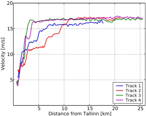
Fig. 2. Ship speed for the recorded tracks. The point of reference in

Tallinn is located at 59◦26.50N, 24◦460E.

but there was some divergence between the results at smaller depths. However, the main features of the wake waves were not altered by the difference in grid resolution. An attempt to reduce the grid size to1x=5 m resulted in severe numerical instabilities due to grid scale noise. As shown by Løvholt and Pedersen (2009), most formulations of the Boussinesq equations contain unstable modes, and the instabilities tend to increase with higher spatial resolution. Løvholt and Ped-ersen (2009) analyzed linear waves and found instabilities due to steep gradients and short oscillations in the water depth. This particular mechanism may not be the most signif-icant for simulations of Tallinn Bay, where bottom slopes are fairly smooth and gentle. However, the combined effect of three-dimensional bathymetric features and nonlinear waves may easily introduce similar unstable modes, requiring an in-crease of dissipative effects in the numerical model to smooth out grid scale noise.

The nearshore of the coastal slope of Tallinn Bay adjacent to the north-bound track (along the Viimsi Peninsula and the western coast of Aegna) usually has a belt of boulders, peb-bles and cobpeb-bles at the shoreline and down to water depths of 0.5–2 m. The seabed in deeper areas, at depths of 2–4 m, typically comprise some cobbles and boulders, interspersed amongst sand and small gravel. The seabed in deeper waters (down to about 15 m) comprises an almost continuous sheet of mixed finer sediments (sand and gravel) with some quite large boulders (∼1 m above seabed) and clusters of boulders (Kask et al., 2003; Parnell et al., 2008). Below 15 m depth the seabed is generally smooth and covered with finer sed-iments. The typical size of bedforms at these depths is a few hundreds of meters (Lutt and Tammik, 1992; Soomere et al., 2007). Such a structure of the bottom usually affects the wave propagation mostly through bottom refraction, which apparently is adequately reflected in simulations. Therefore,

only small-scale features in the immediate nearshore region with a width of less than 1 km may be inadequately repre-sented. The presence of the (small clusters of) boulders evi-dently does not affect the basic properties of the long waves such as the wave period and propagation direction, nor does it cause local wave breaking. However, it obviously leads to a certain damping of wave energy, in particular, in cases when long waves propagate over extensive distances as described above. Bottom friction has been modelled using the classical quadratic form (Lynett et al., 2002)

Rf=

r h+ηu|u|,

where u is the horizontal velocity, h is the water depth, η is the surface displacement, andr is the bottom friction co-efficient. A value ofr=0.02 was used to account for these features by introducing a sufficient level of wave energy dif-fusion in the numerical model. The same value was success-fully used by Pedrozo-Acu˜na et al. (2006) in their study of gravel beaches.

The simulations presented here are based on recent track records for the SuperSeaCat (Fig. 1b), measured during the period of field measurements at Aegna. The tracks were recorded by GPS for two north-bound (track 1 on 29 June 2008 and track 2 on 5 July 2008) and two south-bound (track 3 on 30 June 2008 and track 4 on 5 July 2008) tracks. These records also provide information about the ship ve-locity (Fig. 2) for the four tracks in Fig. 1b. While the two south-bound tracks more or less coincide, there are signif-icant differences between the two north-bound tracks. The reason for the difference is not known, but may be due to traffic or weather conditions.

The water depth at the tripod location varied from 2.5 to 2.8 m, and was close to 2.7 m on the days discussed in this paper. Due to inaccuracies in the digitized topography, the water depth in the numerical model at the tripod location (WG-A in Fig. 1b) was only 1.2 m. The depth at the nearby location WG-4 was 3.9 m, so this wave gauge is more rep-resentative for waves outside the shoaling zone. As the bot-tom isolines at the location of the measurement device are more or less parallel to the crests of the largest ship waves, changes to the wave parameters mostly occur due to shoal-ing, bottom friction and possibly partial breaking. Although the numerical model includes an eddy viscosity model for handling wave breaking, the breaking zone is not resolved in the numerical simulations, and wave breaking was therefore excluded from the simulations.

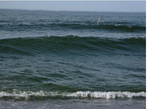
Ship wakes exited in relatively shallow water exhibit group structure where the appearance of the first group very much resembles a typical dispersive open sea wave group. Al-though the group structure is maintained as the waves ap-proach the shore, wave dispersion is significantly reduced in shallow water. The typical length of the first group of a wake from a fast ferry (reduced to the measurement depth of 2.7 m) is about 500–800 m and thus much longer than the dis-tance from the tripod location (or WG-A) to WG-4, and to the runup measurement site (about 100 m). For waves with typi-cal periods of∼10 s the difference of group and phase speed is quite small for this depth. It can therefore be assumed that the particular location of the crest of each wave within a group varies insignificantly between the tripod and the coast, and that individual waves observed during runup correspond to individual waves recorded by the echosounder or numer-ically simulated at WG-A. This assumption was verified vi-sually: in all cases when ship waves were clearly identifiable against the wind wave background (Fig. 3), their crests kept their identity all the way from the tripod to the coast.

3 Simulated wake wave patterns

Wave generation by ships is commonly characterized by the length and depth Froude numbers, defined by

FL=

U

√

gL, FH= U

√

gh,

respectively, where U is the ship speed, g is acceleration of gravity, L is the ship length, and h is the water depth. The wave making resistance has a maximum in the so-called hump speed region 0.4<FL<0.6. For the SuperSeaCat,

which has a length of L=100.30 m, the hump speed re-gion corresponds to velocities in the range from 12.5 m/s to 18.8 m/s, which corresponds to the normal operational speed for this ship (Fig. 2). Shallow water influences both the wave making resistance, which has a maximum near the crit-ical depth Froude numberFH=1, and the shape of the wake

wedge (Soomere, 2007). The apex angle of the Kelvin wedge

Fig. 3. Ship wakes approaching the coast of Aegna.

increases for near critical values ofFH, and transverse waves

moving in the direction of ship propagation disappear in the supercritical regime.

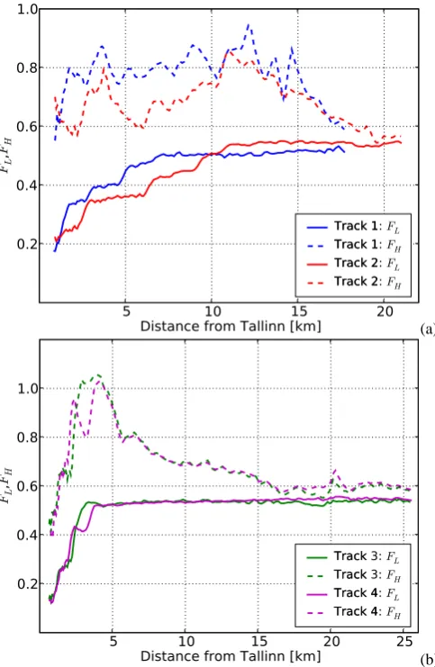
Froude numbers for the two tracks shown in Fig. 1 are shown in Fig. 4. South-bound ships frequently exceed the critical valueFH=1, in the inner part of Tallinn Bay (Torsvik

and Soomere, 2008; Parnell et al., 2008), but they sail at more moderate Froude numbers in the outer part of the bay (Fig. 4). Since the location of the measurement site was largely sheltered from south-bound ship wakes (and wakes which arrived to the site were generated at FH<0.6 in the

outer part of Tallinn Bay), south-bound ship wakes were not prominent in the wave records at Aegna. We will therefore focus only on wakes from the north-bound tracks. North-bound ships often travel at speeds corresponding to a depth Froude number in the range 0.6–0.8 throughout the entire bay. At the same time the length Froude number FL for

SuperSeaCat is in the hump-speed range of 0.4–0.6, where

large amplitude wake waves regularly occur.

5

10

15

20

Distance from Tallinn [km]

0.2

0.4

0.6

0.8

1.0

Track 1

Track 1

Track 2

Track 2

(a)

5

Distance from Tallinn [km]

10

15

20

25

0.2

0.4

0.6

0.8

1.0

Track

Track

Track 4

Track 4

(b)

Fig. 4. Length and depth Froude numbers. (a) north-bound ships; (b) south-bound ships.

Figure 5 shows snap shots of wave patterns generated by the vessel as it is passing Aegna. Although the location of the ships on the panels do not coincide exactly, the figures show mostly qualitatively similar wave patterns, but with some im-portant differences. The wave amplitudes seem to be slightly larger for track 1 (Fig. 5a) than for track 2 (Fig. 5b), which is reasonable given the higher value ofFH for track 1 (Fig. 4).

The largest difference is seen on the coast of Viimsi Penin-sula, where a strong signal is seen in Fig. 5a, but is virtually absent in Fig. 5b. We emphasize that the lowest contour level are at±0.25 m displacement, and that smaller waves are not represented in these figures.

Sailing in sea areas with variable topography is accompa-nied by changes in the nature of the wake pattern both in time and space (Jiang, 2001; Belibassakis, 2003; Jiang et al., 2003; Torsvik et al., 2006). The most impressive changes occur when the ship sails along underwater slopes so that the geometry of the bottom is not symmetric with respect to the sailing line. The overall shape of the resulting wave pattern

Longitude

Latitude

A

(a)

Longitude

Latitude

A

(b)

Fig. 5. Wave patterns from simulations of north-bound leg. Ship

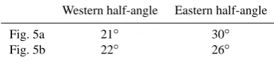
Table 2. Half-angles of the Kelvin wedge for ship wakes in Fig. 5.

Western half-angle Eastern half-angle Fig. 5a 21◦ 30◦ Fig. 5b 22◦ 26◦

(which is symmetric for the classical Kelvin wake for both deep sea and for finite water depth) is then also asymmetric (Belibassakis, 2003). For extensive slopes the half-angle of the corresponding Kelvin wedge on different sides of the fair-way may differ considerably in the vicinity of the ship. This feature, which can be identified from Fig. 5a and b, was mea-sured from the images (Table 2). While the apex angle of the western half of the wake is approximately 21◦–22◦(which is slightly higher than the relevant deep-water value∼19.5◦), the eastern apex half angle is noticeably larger.

The increase of the apex angle of the wake system, even if accompanied by an increase of the largest wave heights, does not necessarily lead to an increase in the wave loads at the coastline. The decisive factor here is the geometry of the coast. For instance, if a section of the coast is oriented so that the distance to the sailing line increases in the sailing direction, then the impact of an increase in wave heights at high Froude numbers is to some extent compensated by an increase in the apex angle. In such a case the extensive wave refraction may lead to a decrease in the amount of ship wave energy per unit length of the shore. This decrease may be one of the reasons why the middle and northern part of the Viimsi Peninsula receives relatively little amount of wake en-ergy (Soomere and Rannat, 2003). Note that the observer at the coast will simply identify a local decrease of the wave in-tensity whereas most of the other wave properties remain the same. An example of a wake “tail” at the coast, where the waves have been redirected and the wave energy is spread along the coast by refraction, can be seen along the northern part of the Viimsi Peninsula in Fig. 5a.

On the other hand, wave loads will experience no decrease for coastal sections that are oriented opposite to the above; for example, the SW coast of Aegna. For such sections the impact of refraction-induced spreading may completely van-ish.

The described asymmetry may considerably increase the variability of the ship-induced wave field in sea areas with complex geometry and bathymetry on top of the features de-scribed in other studies (e.g. the finite extension of the “fan” of ship wakes, Torsvik and Soomere, 2008; Parnell et al., 2008). Our calculations show that energetic wakes excited by the high-speed ferries currently operating in Tallinn Bay most frequently impact the SW coast of Aegna, the coastal section westwards from Tallinn Harbour, and the southern end of Naissaar.

Table 3. Wave periods from measured and simulated wave profiles.

Water Track 1 Track 2

Depth Amplitude Period Amplitude Period

Measurement 2.7 m 0.45 m 10.5 s 0.20 m 8.6 s WG-A 1.2 m 0.49 m 11.7 s 0.11 m 12.4 s WG-1 4.5 m 0.52 m 10.2 s 0.38 m 9.8 s WG-2 2.3 m 0.46 m 12.0 s 0.55 m 12.2 s WG-3 3.3 m 0.74 m 12.3 s 0.19 m 11.7 s WG-4 3.9 m 0.46 m 10.8 s 0.27 m 9.2 s WG-5 2.8 m 0.20 m 11.0 s 0.14 m 8.9 s WG-6 3.3 m 0.23 m 7.0 s 0.06 m 8.7 s

The above analysis suggests that the exact locations of the largest wave loads substantially depend on the Froude num-ber, which affects the geometry of the wake system. The largest waves are expected to occur along specific sections which are oriented almost parallel to ship wave crests at some moderate Froude numbers. For certain sections, changes to the ship wave geometry may even affect the prevailing direc-tion of the ship-wave-induced sediment transport.

4 Numerical simulations and comparison with measurements

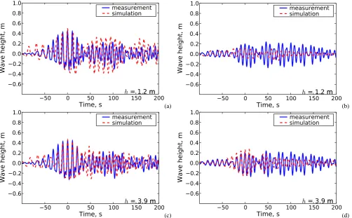
Figure 6 show a comparison between simulated data and wave records at WG-A (59◦34.260N, 24◦45.360E) and at WG-4 (59◦34.120N, 24◦45.330E) (Fig. 1). The mea-sured data has been filtered to remove high frequency noise. The measured and simulated records are aligned so that the largest waves in the first group of large waves (H >1/2HMAX) coincide in both the records. We note again that the depths in the simulations (1.2 and 3.9 m), do not coin-cide with the actual depth at the measurement site (∼2.7 m). The simulated and measured records match fairly well for both tracks in WG-4 (Fig. 6c and d), and also for track 1 in WG-A (Fig. 6a), but the amplitude is too small for the simu-lated result of track 2 in WG-A (Fig. 6b). The group with the largest amplitude waves arrives first, and subsequent wave groups have clearly smaller amplitudes. Although track 2 is located in close proximity to track 1 and the speeds of the vessels along these tracks are almost equal as they pass Aegna, the wake signal is very much different at the mea-surement site. Wave profiles from track 2 differ from track 1, in that the first large wave group has a relatively small am-plitude, and is preceded by a number of smaller amplitude long waves. The amplitude of waves in the first large group are also not significantly larger than in the subsequent groups (Fig. 6b and d).

Time, s

Wave

he

igh

t,m

m

measurement

simulation

(a)

Time, s

Wave

he

igh

t,m

m

measurement

simulation

(b)

Time, s

Wave

he

igh

t,m

m

measurement

simulation

(c)

Time, s

Wave

he

igh

t,m

m

measurement

simulation

(d)

Fig. 6. Comparison between measured and simulated wave profiles. The depth at the measurement site was 2.5 m, and the depth at locations

of virtual wave gauges is indicated in the figures. (a) Track 1: WG-A; (b) Track 2: WG-A; (c) Track 1: WG-4; (d) Track 2: WG-4.

Table 4. Wave period for the leading wave group in Track 2.

Measurement WG-A WG-4 Period 10.4 s 13.0 s 10.2 s

(albeit slightly exceed) the measured wave periods. We also note that WG-4 gives better agreement with the measurement than WG-A, even though the latter wave gauge is located at the measurement site. This result is perhaps not surprising, given the inaccuracies in the bottom topography used in the simulations. Given the differences in depth between WG-4 and WG-A one could have expected to see some indication of wave shoaling, but this effect has been countered by dis-sipative effects due to the bottom friction model and numer-ical dissipation inherent in the time stepping scheme of the model.

The results in Table 3 exaggerate the difference in wave period between the two recordings because the highest waves at different gauges correspond to different parts of the wake. Table 4 shows estimates for the wave period of the leading wave group for track 2, which shows that the periods of these waves were consistently larger than 10 s.

Time, s

Wave

he

igh

t,m

m

29.06.08

05.07.08

(a)

Time, s

Wave

he

igh

t,m

m

29.06.08

05.07.08

(b)

Time, s

Wave

he

igh

t,m

m

29.06.08

05.07.08

(c)

Time, s

Wave

he

igh

t,m

m

29.06.08

05.07.08

(d)

Time, s

Wave

he

igh

t,m

m

29.06.08

05.07.08

(e)

Time, s

Wave

he

igh

t,m

m

29.06.08

05.07.08

(f)

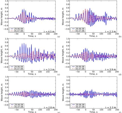
Fig. 7. Comparison between simulated wave profiles at wave gauges 1–6. (a) WG-1; (b) WG-2; (c) WG-3; (d) WG-4; (e) WG-5; (f) WG-6.

Obviously, the large differences between wave records at some wave gauges have their origin in the different speeds and tracks of the ships, and far more tracks should be sim-ulated to get realistic statistics to work with. Interplay of wakes and bedforms may create zones of wave focusing, where waves from different parts of the wake “fan” merge. Even if these locations are well known, a slight variation in a ship track may change the sites that the wake waves reach simultaneously.

Some of the wave profiles (Figs. 6c, 7c) show a complex wave field which may stem from a superposition of two wave fields originating from different parts of the wake “fan”. It

has been suggested that a ship may generate particularly large waves during acceleration when it remains in the near-critical regime for a long time (Torsvik et al., 2006; Torsvik and Soomere, 2008). Since there are considerable differences in the speed profiles of the two tracks (Fig. 2), this effect may also contribute to the observed differences in the ship wakes.

5 Observed results of wave runup

0 1 2 3 4 5 −0.5

0 0.5 1

Time (min)

Sea level, runup (m)

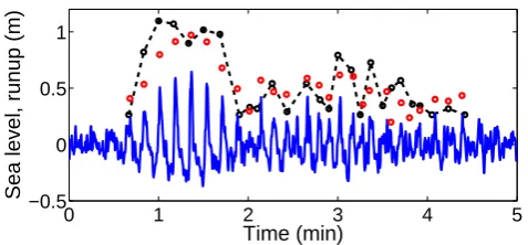
Fig. 8. Waves measured at the tripod (solid line) and the wave

height measured at the runup stage (dashed line). The red circles correspond to the heights of the waves at the tripod, which produce runup on a beach.

finite volume sources that change the volume of the water column above the source area and thus create a flux of water carried by the wave. This similarity is due to the fact that ships sailing in the near-critical regime usually create an ex-tensive, long-living depression area in the vicinity of the ship (Grimshaw and Smyth, 1986; Jiang, 2001; Gourlay, 2006; Soomere, 2007).

It is commonly thought that ship-induced solitons are re-sponsible for the transport of the water from the depression area to the far-field. As the amplitude of such solitons is very small in open sea areas, the highest (equivalently, the most nonlinear) waves of the ship’s wake could be equally respon-sible for such transport. The excess water carried by such waves may considerably impact the runup properties of the waves when the runup process occurs on top of a temporar-ily increased water level at the coast, or on the background of flow of the wave-carried water to the coast and the backwash of this excess water.

As an example of runup measurements, we analyze data from 29 June when the simulated and measured wave prop-erties for track 1 well match each other. This day was not per-fectly calm, but still offered reasonable conditions for runup recordings and, in particular, for comparisons of the runup of wind and ship waves of comparable height.

Wind waves and ship waves were usually clearly distin-guished on calm days as well as on days with the signifi-cant wave height of the natural waves below 50–60 cm. Wind waves with the height of up to 0.5 m produced runup events up to 20–30 cm above the still water level, with the runup usually clearly smaller than the wave height. In general, the runup of ship waves with a height of about 1 m frequently reached well over 1 m above the still water level. A few waves (not necessarily the highest) went over the berm crest located>1.5 m above the still water level. In calm condi-tions, the ship wave runup process usually started with a significant rundown. This phenomenon was probably con-nected with the presence of precursor solitons. Subsequently a group of about 10 large-amplitude waves reached the coast. The typical length of these large waves varied from 40 to

80 m (Fig. 3). A more detailed description of the features of the ship wave runup can be found in (Parnell et al., 2008).

A comparison of the measured waves at the tripod and runup heights on a beach for the wake from track 1 on 29 June is presented in Fig. 8. The recordings at the tripod (solid line) and measurements on the beach (dashed line) are matched by the time period of the first group of waves. The red circles correspond to the heights of the waves at the tri-pod, which produce runup on a beach. These waves are as-sumed to be the largest waves, recorded at the tripod that fall within the time intervals defined by two consecutive wave runups on the beach. It follows from Fig. 8 that the runup recordings miss a few initial waves of the wake, the runup of which probably was not noticeable to the observers. As expected, the largest runup heights correspond to the group of largest waves of the wake. The runup pattern has a group structure similar to the wake, with a clearly distinguishable low runup between the first group of the highest waves and the second group of somewhat smaller but still significant waves (see Parnell et al., 2008). While the very first waves, waves between the two groups, and waves at the very end of the wake produce runup almost equivalent to their mea-sured heights, several waves (mostly the middle ones of the groups) produce much larger runup values than one might expect based on the wave height. As the periods of waves gradually decrease with time in both groups (Soomere and Rannat, 2003; Parnell et al., 2008), Fig. 8 confirms that the difference in wave periods cannot explain the difference in their runup heights. The excess of water carried to the site ei-ther by precursor solitons or by the relatively long first wave group might be an explanation why runup of these waves is unexpectedly high.

This feature is further illustrated by means of a scatter dia-gram of measured wave heights and the corresponding runup (Fig. 9). The dotted line in Fig. 9 is simply the diagonal. The dashed line corresponds to Hunt (1959) empirical for-mula, which determines runup as a function of beach slopeα (α=0.027 for the beach of Aegna), incident wave heightH, and wave steepness based on laboratory data and explains the behavior of low-height breaking waves, the surf simi-larity parameter for which is 0.1<ξ <2.3 (in our experiment ξ∼0.6):

R=H ξ , ξ=αpλd/Hd, (1)

whereHd is the wave height and λd is the wavelength of

0 0.4 0.8 1.2 0

0.4 0.8 1.2

Wave height (m)

Runup height (m)

Fig. 9. Scatter diagram of wave heights measured at the tripod and

at the runup stage. The dotted line is the diagonal, the dashed line corresponds to Hunt (1959) Eq. (1), and the solid line corresponds to Eq. (2), given by Massel and Pelinovsky (2001).

R=2H

2

J0()−i√1+iγ J1()

, (2)

=2ω

s

(1+iγ )L

αg , γ=0.937 δ πα

0.155

_H

d

λd

−0.13

,

whereLis a distance from the wave to the shoreline (L=100 m in the experiment),ωis a wave frequency, andδis an ex-perimental parameter of the order one (δ=1 is used in Fig. 9). The distribution of the height and runup properties of different waves in Fig. 9 suggests that the set of recorded waves can be divided into three classes. About a half of the waves, mostly the shortest waves from those forming the ship wake, produce runup heights of 20–40 cm. Their runup does not significantly depend on the wave height. These low-height breaking waves (stars in Fig. 9) can be described by means developed by Hunt (1959) Eq. (1). The second group of (medium-height) waves, mostly representing the highest waves of the second group of the wake (cf. Soomere, 2007), generally produce larger runup than their heights. The em-pirical relation between their heights and runup properties (circles in Fig. 9) is in good agreement with Eq. (2), given by Massel and Pelinovsky (2001). The most interesting group are the highest waves of the first group of the wake (squares in Fig. 9), which are usually breaking waves. The presented results suggest that their runup height can be described nei-ther by Eq. (1) nor (2). As mentioned above, their excess runup height may be connected with the excess water carried to the coast by these evidently nonlinear waves.

0 5 10 15

0 5 10 15

Wave period (s)

Runup period (s)

Fig. 10. The scatter diagram of periods of waves measured at the

tripod and at the runup stage. The dotted line is the diagonal.

Partial wave breaking in the nearshore changes to some extent the observed properties of the waves at the runup mea-surement site. In realistic conditions, some (usually shorter and/or smaller) waves from the wave group partially break before they reach the coast. This phenomenon may be con-nected with intense backwash from preceding waves. If smaller waves follow a large wave, the backwash of the larger wave may completely mask runup of the smaller waves. Therefore, it is not unexpected that the number of waves cre-ating measurable runup is smaller than the number of waves measured at the tripod.

Figure 10 shows the scatter diagram of peak-to-peak peri-ods of waves measured at the tripod and at the runup stage. The periods of the waves at the beach can be taken directly from the measurements, and the corresponding wave period from the tripod is found by taking the peak-to-peak period between the largest wave within the time interval defined by two consecutive runup events, and the largest preceding wave. The wave heights of the waves at the tripod used in Fig. 10 are marked as red circles in Fig. 8. It follows from Fig. 10 that the periods of the waves at the tripod and at the runup stage are in a good agreement. Thus, the ship waves usually do not merge and each runup record reflects the prop-erties of a single ship wave.

6 Concluding remarks

quantitative features of the remote field of ship wakes using a numerical model. Simulated wave periods mostly well match (albeit tend to slightly exceed) the measured values. The reasonable choice of the parameters of the numerical scheme reflecting local properties of the seabed leads to overall re-liable estimates of the local ship wave heights in the coastal zone, even at a distance of several kilometres from the sailing line.

Our analysis suggests that the largest differences between the simulated and measured wake properties (equivalently, uncertainties in estimates of the wave heights) frequently stem from an inexact representation of the spatial extension of the high ship waves. The latter is the most sensitive param-eter of the ship wake, the detailed properties of which depend on both sailing regime and local topography. The uncertain-ties stemming from the spatial variability of the extension of ship wakes may lead to an underestimation of the potential ship wave loads by an order of magnitude. An exact nu-merical forecast of extreme ship wake conditions, therefore, needs not only a more detailed topography in order to im-prove the quality of the forecast, but also a large number of simulations for variations in the sailing line and perhaps even variations of topography in order to account for the poten-tial changes to the spapoten-tial extent of the wake pattern. Other features may also be improved, such as including a realistic wave breaking model, or perhaps including filtering of high frequencies in the near shore region, in order to reduce the generation of high frequency waves in the shoaling zone. The representation of the ship may be improved as well, but it is not clear that this would significantly improve the prediction of wave conditions at the coast.

The results show a significant variability in the ship wake profiles in the near shore region. There is both a spatial variability for each individual track, and variability between different tracks. However, there seems to be some general trends in the occurrence of extreme waves at the coast, as seen when comparing locations further east of WG-A with locations further west.

There is a clear correlation between the offshore wave height and the runup height. However, the records suggest that the relationship between runup height and the parame-ters of particular waves and perhaps even the particular loca-tion of a single wave in a group is very complex.

Due to the large variability shown in the data, performing extensive field studies and the use of statistical methods will be essential in further analysis of the ship wake properties. This is achievable with the existing wave records and runup data at a single point (Parnell et al., 2008), but there is a clear lack of data about the properties of spatial variability of ship waves connected with the variations of ship tracks.

As ship wake events consist of a multitude of different wave forms, such as essentially perfect solitons, highly non-linear, almost solitonic cnoidal waves, strongly asymmetric waves, and almost sinusoidal entities (Soomere et al., 2005; Parnell et al., 2008), they may provide an excellent means

by which to further our understanding of the relationship be-tween different wave types and coastal processes.

Acknowledgements. This research is supported by Marie Curie

network SEAMOCS (MRTN-CT-2005- 019374), EEA grant (EMP41), ESF grant 7413, Estonian block grant SF0140077s08, and RFBR grants (08-02-00039, 08-05-00069, 08-05-91850). Two authors (TT and KEP) received support from the Marie Curie Transfer of Knowledge project CENS-CMA (MC-TK-013909) while visiting the Centre for Nonlinear Studies. We are grateful for the contributions from T. Dolphin, who recorded the ship tracks on 29 June 2008.

Edited by: R. Grimshaw

Reviewed by: two anonymous referees

References

Belibassakis, K. A.: A coupled-mode technique for the transforma-tion of ship-generated waves over variable bathymetry regions, Appl. Ocean Res., 25, 321–336, 2003.

Didenkulova, I. and Pelinovsky, E.: Run-up of long waves on a beach: the influence of the incident wave form, Oceanology, 48(1), 1–6, 2008.

Didenkulova, I., Zahibo, N., Kurkin, A., Levin, B., Pelinovsky, E., and Soomere, T.: Runup of nonlinearly deformed waves on a coast, Dokl. Earth Sci., 411(8), 1241–1243, 2006.

Didenkulova, I., Kurkin, A., and Pelinovsky, E.: Run-up of solitary waves on slopes with different profiles, Izvestiya, Atmospheric and Oceanic Physics, 43(3), 384–390, 2007a.

Didenkulova, I., Pelinovsky, E., Soomere, T., and Zahibo, N.: Runup of nonlinear asymmetric waves on a plane beach, in: Tsunami & Nonlinear Waves, edited by: Kundu, A., Springer, 175–190, 2007b.

Gourlay, T. P.: A simple method for predicting the maximum squat of a high-speed displacement ship, Mar. Technol. Soc. J., 43, 146–151, 2006.

Grimshaw, R. H. J. and Smyth, N.: Resonant flow of a stratified flow over topography, J. Fluid Mech., 169, 429–464, 1986. Hunt, J. A.: Design of seawalls and breakwaters, J. Waterw. Port C.

Div., 85, 123–152, 1959.

Jiang, T.: Ship waves in shallow water, VDI Verlag, D¨usseldorf, Fortschritt-Berichte VDI, Reihe 12, Nr. 466, 152 pp., 2001. Jiang, T., Henn, R., and Sharma, S. D.: Wash waves generated by

ships moving on fairways of varying topography, in: Proceedings for the 24th Symposium on Naval Hydrodynamics, Fukuoka, 8– 13 July 2002, National Academy Press, Washington DC, 441– 457, only available at: www.nap.edu, 2003.

Kask, J., Talpas, A., Kask, A., and Schwarzer, K.: Geological set-ting of areas endangered by waves generated by fast ferries in Tallinn Bay, Proc. Estonian Acad. Sci. Eng., 9, 185–208, 2003. Liu, P. L.-F. and Wu, T.-R.: Waves generated by moving pressure

disturbances in rectangular and trapezoidal channels, J. Hydraul. Res., 42, 163–171, 2004.

Lindholm, T., Svartstr¨om, M., Spoof, L., and Meriluoto, J.: Effects of ship traffic on archipelago waters off the L˚angn¨as harbour in

˚

Aland, SW Finland, Hydrobiologia, 444, 217–225, 2001. Lutt, J. and Tammik, P.: Bottom sediments of Tallinn Bay, Proc.

Lynett, P. and Liu, P. L.-F.: A numerical study of submarine land-slide generated waves and runup, P. Roy. Soc. Lond. A, 458, 2885–2910, 2002.

Lynett, P., Wu, T.-R., and Liu, P. L.-F.: Modeling wave runup with depth-integrated equations, Coast. Eng., 46, 89–107, 2002. Løvholt, F. and Pedersen, G.: Instabilities of Boussinesq

models in non-uniform depth, Int. J. Numer. Meth. Fl., doi:10.1002/fld.1968, in press, 2009.

Massel, S. and Pelinovsky, E.: Run-up ofdispersive and breaking waves on beaches, Oceanologia, 43(1), 61–97, 2001.

Mathew, J. and Akylas, T. R.: On three-dimensional long water waves in a channel with sloping sidewalls, J. Fluid Mech., 215, 289–307, 1990.

Miles, J. W.: Obliquely interacting solitary waves, J. Fluid Mech., 79, 157–169, 1977.

Parnell, K. E. and Kofoed-Hansen, H.: Wakes from large high-speed ferries in confined coastal waters: Management ap-proaches with examples from New Zealand and Denmark, Coast. Manage., 29, 217–237, 2001.

Parnell, K., Delpeche, N., Didenkulova, I., Dolphin, T., Erm, A., Herrmann, H., Kask, A., Kelpsaite, L., Kurennoy, D., Quak, E., R¨a¨amet, A., Soomere, T., Terentjeva, A., Torsvik, T., and Zaitseva-P¨arnaste, I.: Far-field vessel wakes in Tallinn Bay, Es-tonian J. Eng., 14(4), 273–302, 2008.

Pedrozo-Acu˜na, A., Simmonds, D. J., Otta, A. K., and Chadwick, A. J.: On the cross-shore profile change of gravel beaches, Coast. Eng., 53, 335–347, 2006.

Peterson, P., Soomere, T., Engelbrecht, J., and van Groesen, E.: Soliton interaction as a possible model for extreme waves in shal-low water, Nonlin. Processes Geophys., 10, 503–510, 2003, http://www.nonlin-processes-geophys.net/10/503/2003/. PIANC: Guidelines for managing wake wash from high-speed

ves-sels, report of the Working Group 41 of the Maritime Navi-gation Commission, International NaviNavi-gation Association (PI-ANC), Brussels, 2003.

Sitanggang, K. and Lynett, P.: Parallel computation of a highly non-linear Boussinesq equation model through domain decomposi-tion, Int. J. Numer. Meth. Fl., 49, 57–74, 2005.

Soomere, T.: Fast ferry traffic as a qualitatively new forcing factor of environmental processes in non-tidal sea areas: a case study in Tallinn Bay, Baltic Sea, Environ. Fluid Mech., 5, 293–323, 2005. Soomere, T.: Nonlinear components of ship wake waves, Appl.

Mech. Rev., 60, 120–138, 2007.

Soomere, T. and Rannat, K.: An experimental study of wind waves and ship wakes in Tallinn Bay, Proc. Estonian Acad. Sci. Eng., 9, 157–184, 2003.

Soomere, T., P˜oder, R., Rannat, K., and Kask, A.: Profiles of waves from high-speed ferries in the coastal area, Proc. Estonian Acad. Sci. Eng., 11, 245–260, 2005.

Soomere, T., Kask, A., Kask, J., and Nerman, R.: Transport and dis-tribution of bottom sediments at Pirita Beach, Estonian J. Earth Sci., 56, 233–254, 2007.

Torsvik, T. and Soomere, T.: Simulation of patterns of wakes from high-speed ferries in Tallinn Bay, Estonian J. Eng., 14, 232–254, 2008.

Torsvik, T., Dysthe, K., and Pedersen, G.: Influence of variable Froude number on waves generated by ships in shallow water, Phys. Fluids, 18, 062102, doi:10.1063/1.2212988, 2006. Torsvik, T., Pedersen, G., and Dysthe, K.: Influence of cross

chan-nel depth variation on ship wave patterns, E-print series, Me-chanics and Applied Mathematics No. 2, Dept. of Math., Univer-sity of Oslo, Norway, ISSN 0809-4403, August 2008.