A multi method autonomous assessment of primary productivity and export efficiency in the springtime North Atlantic

https://doi.org/10.5194/bg-15-4515-2018 © Author(s) 2018. This work is distributed under the Creative Commons Attribution 4.0 License.

A multi-method autonomous assessment of primary productivity

and export efficiency in the springtime North Atlantic

Nathan Briggs1, Kristinn Guðmundsson2, Ivona Cetini´c3,4, Eric D’Asaro5, Eric Rehm6, Craig Lee5, and Mary Jane Perry7

1_{National Oceanography Centre, Southampton SO14 3ZH, UK} 2_{Marine Research Institute, P.O. Box 1390, 121 Reykjavík, Iceland}

3_{GESTAR/Universities Space Research Association, 7178 Columbia Gateway Drive, Columbia, MD 21046, USA} 4_{Ocean Ecology Laboratory, NASA Goddard Space Flight Center Code 616, Greenbelt, MD 20771, USA} 5_{Applied Physics Laboratory and School of Oceanography, University of Washington, Seattle, WA 98105, USA} 6_{Département de Biologie et Québec-Océan, Université Laval, Québec QC G1V 0A6, Canada}

7_{Darling Marine Center, School of Marine Sciences, University of Maine, Walpole, ME 04573, USA}

Correspondence:Nathan Briggs ([email protected]) Received: 12 December 2017 – Discussion started: 4 January 2018

Revised: 18 May 2018 – Accepted: 29 May 2018 – Published: 25 July 2018

Abstract. Fixation of organic carbon by phytoplankton is the foundation of nearly all open-ocean ecosystems and a critical part of the global carbon cycle. But the quantifica-tion and validaquantifica-tion of ocean primary productivity at large scale remains a major challenge due to limited coverage of ship-based measurements and the difficulty of validating diverse measurement techniques. Accurate primary produc-tivity measurements from autonomous platforms would be highly desirable due to much greater potential coverage. In pursuit of this goal we estimate gross primary productivity over 2 months in the springtime North Atlantic from an au-tonomous Lagrangian float using diel cycles of particulate organic carbon derived from optical beam attenuation. We test method precision and accuracy by comparison against entirely independent estimates from a locally parameterized model based on chlorophyllaand light measurements from the same float. During nutrient-replete conditions (80 % of the study period), we obtain strong relative agreement be-tween the independent methods across an order of magnitude of productivities (r2=0.97), with slight underestimation by the diel cycle method (−19±5 %). At the end of the diatom bloom, this relative difference increases to −58 % for a 6-day period, likely a response to SiO4limitation, which is not

included in the model. In addition, we estimate gross oxygen productivity from O2diel cycles and find strong correlation

with diel-cycle-based gross primary productivity over the

entire deployment, providing further qualitative support for both methods. Finally, simultaneous estimates of net commu-nity productivity, carbon export, and particle size suggest that bloom growth is halted by a combination of reduced produc-tivity due to SiO4limitation and increased export efficiency

due to rapid aggregation. After the diatom bloom, high Chl a-normalized productivity indicates that low net growth during this period is due to increased heterotrophic respiration and not nutrient limitation. These findings represent a significant advance in the accuracy and completeness of upper-ocean carbon cycle measurements from an autonomous platform.

1 Introduction

availabil-ity. Understanding is further limited by the difficulty in vali-dating PP, as each method has potential sources of bias, but generally no two methods measure the exact same quantity at the same temporal scale. Therefore, it is often unclear whether discrepancies between independent measurements are caused by biases or real differences. Satellite PP algo-rithms and global models can achieve the desired coverage, but these products still must be validated, ideally using an in situ dataset of confirmed accuracy that spans many years in all seasons and in all oceans. Autonomous platforms can achieve such in situ coverage at a fraction of the cost of ship-based sampling, so the ability to estimate PP from an autonomous platform and validate these estimates using in-dependent methods is highly desirable, both for directly en-hancing the understanding of ocean ecosystems and validat-ing the models and satellite products that can approach true continuous global coverage.

Methods for estimating PP from diel cycles in particu-late beam attenuationcp(Siegel et al., 1989; Claustre et al.,

1999; Cullen et al., 1992; Kinkade et al., 1999; Marra, 2002; Dall’Olmo et al., 2011; Gernez et al., 2011; Omand et al., 2017; White et al., 2017) or O2(Caffrey, 2003; Hamme et

al., 2012; Nicholson et al., 2015) are suited for application to autonomous platforms, many of which already carry O2

sensors and/or transmissometers. These methods rely on the light dependence of PP, which causes a diel cycle in O2and

incp(due to its correlation with particulate organic carbon,

POC). However, other factors, such as zooplankton vertical migrations, mixing events, O2air–sea flux, and POC/ cp

ra-tios, may have diel cycles that introduce bias in these PP estimates, so they cannot be relied upon without validation. Comparisons so far between diel cycles and independent PP estimates have been encouraging, generally agreeing within a factor of 2 to 3 (Cullen et al., 1992; Walsh et al., 1995; Kinkade et al., 1999; Hamme et al., 2012; Nicholson et al., 2015), but the independent estimates have not been of the same quantity at the same temporal scale, so these compar-isons do not provide strong constraints on the accuracy of this method.

In this study we take three significant steps towards the goal of enhancing our understanding of ocean ecosystems by increasing coverage of accurate in situ PP estimates using autonomous platforms. First, we use diel cycles in measure-ments of cpand O2to simultaneously estimate two related

quantities, the gross primary productivity (GPP) of particu-late organic carbon and gross oxygen productivity (GOP), in the surface mixed layer over a 2-month period from an au-tonomous Lagrangian float. Two our knowledge, this is the first time that cp-based GPP and GOP have been

simulta-neously calculated using diel cycles from any platform, let alone autonomously. Second, we compare our diel-cycle-based GPP estimates with entirely independent estimates of the same quantity at the same spatial and temporal scale across a wide dynamic range of productivities. Again, to our knowledge, this represents the most rigorous validation of the

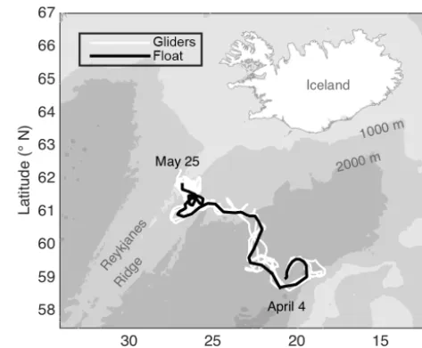
Figure 1.Study area with tracks of an autonomous Lagrangian mixed-layer float and autonomous Seagliders.

diel cycle method to date. Third, we apply our mixed-layer PP estimates, in conjunction with mixed-layer O2, NO3, and

POC budgets, to better understand how PP, heterotrophic res-piration, and sinking flux all interact to regulate mixed-layer biomass in our study system: the spring diatom bloom in the Iceland Basin.

2 Methods

2.1 Study area and platforms

The data presented here were collected by an autonomous Lagrangian mixed-layer float, two ships, and three au-tonomous Seagliders during the North Atlantic Bloom 2008 (NAB08) project. All data used here are available online at http://www.bco-dmo.org/project/2098, last access: 23 July 2018. The float was deployed on 4 April in the Iceland Basin at 59◦N, 20.5◦W near the 60◦N site of the 1989 Joint Global Ocean Flux Study (JGOFS). The NAB08 project centered around the float, which was designed to drift in the surface mixed layer, mimicking the movement of plank-ton, except for daily profiles to 250 m (D’Asaro, 2003). The float gathered data for 2 months, drifting northwest towards the Reykjanes Ridge, ceased collecting data on 25 May at 61.8◦_{N, 26.7}◦_{W (Fig. 1; black line), and was recovered on} 3 June. The timing of the daily float profiles was irregu-lar until 14 April, after which the float profiled each day between 15:00 GMT and dusk. The float carried an array of sensors, including two SBE 43 CTs for temperature and salinity, a WET Labs C-Star transmissometer for particu-late organic carbon (POC) via particuparticu-late beam attenuation cp, a WET Labs FLNTU (fluorescence and turbidity

optical backscatteringbbp, a Sea-Bird SBE 43 and an

Aan-deraa optode for oxygen, an ISUS (in situ ultraviolet spec-trophotometer) for NO3, and a LI-COR LI-192SA for planar

photosynthetically active radiation (PAR). See Appendix A for a list of abbreviations used in more than one subsection. Three cruises provided calibration data for the float’s sensors as well as more detailed biological and chemical measure-ments: a deployment cruise by the RVBjarni Saemundsson

(3–5 April), a process cruise by the RVKnorr(2–21 May), and a float “rescue” cruise by the RV Bjarni Saemundsson

(4–5 June). The ships collected both in situ measurements and discrete water samples via an overboard CTD package, which profiled to 600 m. Both ships carried the same array of in situ sensors as the float, minus the ISUS NO3 sensor

and the Aandera optode. In addition, the RV Knorrcarried a second CTD and an above-water PAR sensor. Unlike the float, both of the ship’s PAR sensors measured scalar PAR. The Seagliders were deployed together with the float and pi-loted to follow it throughout the experiment. Over the de-ployment, the distance between the float and individual glid-ers ranged from 175 to<1 km. However, at least one glider was within 50 km of the float for almost the entire deploy-ment, and starting on 6 May, all gliders remained within 50 km. Seagliders carried an array of sensors, but here we only discuss Seaglider estimates of sinking flux, derived in Briggs et al. (2011) using spikes caused by large particles in bbp, which was measured by a WET Labs BB2F.

2.2 Discrete sampling

Discrete samples from all three cruises were analyzed at depths ranging from near surface (3–5 m) to 600 m for particulate organic carbon (POC; n=343), chlorophyll a (Chl a; n=935), SiO4 and NO3 (n=1001), and

phy-toplankton pigments (n=80). Detailed methodology for these analyses can be found in the following technical re-port: http://data.bco-dmo.org/NAB08/Laboratory_analysis_ report-NAB08.pdf, last access: 23 July 2018. Briefly, Chla samples were filtered onto GFF 0.7 µm filters and analyzed onboard using a Turner Designs model 10AU fluorome-ter. Following JGOFS protocols, POC samples were filtered onto precombusted GFF 0.7 µm filters, sealed in foil pack-ets, and stored at −20◦C until analysis onshore using a Perkin Elmer 2400 CHN analyzer. For nutrients, 60 mL sam-ples were immediately frozen and stored at −20◦C until analysis onshore using a Latchat Quickchem 8000 Flow In-jection Analysis System. In addition, discrete samples on the May process cruise were analyzed for dissolved oxy-gen concentration via Winkler titrations (n=131) and for bacterial counts and phytoplankton community composition using a FACScan flow cytometer and a FlowCAM auto-mated microscopic imager. Phytoplankton particles were di-vided into several groups based on optical properties, size, and morphology as described in Cetini´c et al. (2012), with more detailed methods in a technical report accompanying

the dataset: http://data.bco-dmo.org/NAB08/Phytoplankton_ Carbon-NAB08.pdf, last access: 23 July 2018.

2.3 Calibration of in situ sensors

The ship’s profiler was held at constant depth for 60 s prior to closing each bottle to capture a water sample. In situ mea-surements from the 30 s prior to bottle closing were aver-aged to obtain a single value for matchups with discrete sam-ples. Ship in situ sensors were calibrated via linear regression against discrete measurements. Float in situ sensors were cal-ibrated using data from 10 calibration casts during which the ship was brought to the float’s location and simultane-ous ship and float profiles were conducted. Float NO3 and

oxygen sensors were calibrated directly against the discrete measurements taken during the calibration casts. All other float sensors were calibrated against the matching ship in situ sensors in order to maximize the number of matchups. Individual calibration details for each float sensor are listed below.

2.3.1 Temperature and salinity

The duplicate temperature (T) and salinity (S) sensors aboard the ship’s profiler during the May process cruise agreed closely (median S difference ≤0.0018 and a me-dianT difference≤0.0006◦C for each of 134 profiles). The shipT S sensors were therefore used as standards, after de-spiking and averaging (more details at http://data.bco-dmo. org/NAB08/Ship_TS_despiking-NAB08.pdf, last access: 23 July 2018). DuplicateT sensors aboard the float also agreed closely and were therefore combined into a single record without adjusting to match the ship. After reconciliation of duplicate S measurements on each platform, a small mis-match between float and ship salinity was identified from the calibration casts and corrected by subtracting 0.0075 from the float S (more details at http://data.bco-dmo.org/ NAB08/CTD_float_Calibration-NAB08.pdf, last access: 23 July 2018).

2.3.2 Oxygen

May 1 May 10 May 20

POC / c

p

(mmol C m

-2)

0 10 20 30 40 50 60 70 80 90 100

Out of patch In float patch Float patch fit

Figure 2.POC/ cpfrom the May cruise in the upper 30 m and the

fit used to calculate POCcp.

bco-dmo.org/NAB08/Oxygen_Calibration-NAB08.pdf, last access: 23 July 2018.

2.3.3 POC from optical beam attenuation

Previous work has shown that measurements of light scat-tering by particles, including beam attenuation cp and

par-ticulate backscattering bbp, correlate strongly with POC in

the open ocean (Cetini´c et al., 2012, and references therein). Calibration of our cp and bbp measurements and

conver-sion to POC estimates are described in the next two sub-sections. Raw output from the float optical beam transmis-someter was aligned with raw ship transmistransmis-someter out-put using matchups from eight of the calibration casts. Agreement was very good (r2=0.99), showing no evi-dence of sensor drift. Intercalibrated raw transmissome-ter output was converted to particulate optical beam at-tenuation cp using the mean of factory calibrations

per-formed on the ship’s transmissometer before and after de-ployment. More details can be found at http://data.bco-dmo. org/NAB08/C-Star_Calibration-NAB08.pdf, last access: 23 July 2018. We estimated cp-derived POC (POCcp)

follow-ing Cetini´c et al. (2012), but with a time-dependent adjust-ment in POC/ cp ratio to account for community changes.

After subtracting the POC/ cpregression offset of 0.015 m−1

(Cetini´c et al., 2012) from our cp measurements, we

com-puted the POC/ cpratio for all ship POC andcpsamples for

whichcp>0.2 m−1in the upper 30 m during the May

pro-cess cruise (Fig. 2; gray points). Samples whose T,S,cp,

andbbpmatched the float ML measurements within 0.25◦C,

0.01 m−1, 0.1 m−1, and 0.001 m−1, respectively, are shown as black circles (Fig. 2). Three inflection points were fit by eye at 370, 310, and 450 mg m−2on 6, 11, and 15 May, re-spectively. A continuous estimate of POC/ cp at the float

patch was obtained by interpolating between these points and

assuming constant POC/ cpbefore 6 May and after 15 May

(Fig. 2, red line). This continuous estimate of POC/ cpwas

multiplied by floatcp(minus offset of 0.015 m−1) to yield a

cp-based float POC estimate (POCcp).

2.3.4 POC from optical backscattering

An average of pre- and post-deployment calibrations was used to convert raw backscattering output from both the float and the ship to the volume-scattering function at the angle (140◦) and wavelength (700 nm) of the sensors. The volume-scattering function of seawater was then calculated following Zhang et al. (2009) and subtracted to yield scat-tering due to particles. The result was multiplied by 2π χ to yield the particulate backscattering coefficientbbp, where

the angle-dependent scale factorχ is 1.132 for the FLNTU scattering sensors used in this study (Michael Twardowski, personal communication, 2010). Floatbbpwas aligned with

shipbbp using matchups from eight calibration casts (r2=

0.96). More details can be found at http://data.bco-dmo.org/ NAB08/Backscatter_Calibration-NAB08.pdf, last access: 23 July 2018. Gliderbbpwas calibrated against the ship FLNTU

in a similar fashion to the float (Briggs et al., 2011). We estimated bbp-derived POC (POCbbp) following Cetini´c et

al. (2012) via the equation POCbbp[mg C m−3]=37 500bbp

[m−1]−14, derived from a linear regression between colo-cated measurements of POC andbbpwithin the mixed layer

from the May process cruise. 2.3.5 Chlorophylla

Raw chlorophyll fluorometer output from the ship was con-verted to an initial Chl a estimate Chl afactory using the

factory-calibrated scale factor and a dark offset derived from the minimum of all per-cast deep values (defined as the median between 550 and 580 m). An empirical fit between Chlafactory,T, PAR, and ship discrete Chla measurements

was used to derive an in situ Chlaproduct

Chla=Chlafactory·

2.1×10(T−9.2)·0.8+0.44 10(T−9.2)·0.8+1

·

log₁₀(PAR)·0.05+1.02

·tanhPAR₉₅ ·0.55 0.55·PAR

95

, (1)

which was strongly correlated with discrete Chl a (r2=

0.87). Float Chl afactory was aligned with ship Chl afactory,

continuous, depth-resolved record of Chl a for the calcula-tion of primary productivity, the remaining Chla estimates, from both mixed-layer mode and profiles, were filtered us-ing a 5-point runnus-ing median, averaged in 1 h, 1 m bins, and then interpolated in depth and time via triangulation-based 2-D linear interpolation, with distance calculated as

p

(dz[m]/30[m])2_+dt[days]2_{(i.e., a 30 m vertical interval}

and a 1-day time interval were considered equidistant). 2.3.6 Nitrate

A post-deployment laboratory calibration, including temper-ature and salinity corrections, was used to obtain initial NO3

estimates from the float’s ISUS NO3 sensor. An additional

scale factor of 1.15 and offset of +2.6 µM were required to bring these initial estimates in line with discrete samples taken during calibration casts. More details can be found in Alkire et al. (2012) and at http://data.bco-dmo.org/NAB08/ ISUS_Nitrate_Calibration-NAB08.pdf, last access: 23 July 2018.

2.3.7 Silicate

SiO4 was not measured by the float, but discrete

ship-board SiO4 measurements from the top 15 m were

consid-ered to represent mixed-layer SiO4 at the float location if

the corresponding temperature, salinity, and NO3

measure-ments matched concurrent float ML measuremeasure-ments to within 0.25◦C, 0.01, and 0.8 mmol m−3, respectively.

2.3.8 PAR

The factory calibration of the float PAR sensor was used “as is.”

2.4 Mixed-layer depth

Mixed-layer depth (MLD) was calculated at hourly inter-vals from float potential density anomaly estimates via the following steps. (1) Smooth density time series using a 5-point running median. (2) Average density into 1 h, 1 m bins. (3) Fill in the gaps with 2-D linear interpolation such that a 30 m vertical interval and a 1-day time interval are con-sidered equidistant. (4) For each hour, find the minimum potential density anomaly. (5) The MLD for each hour is defined as the shallowest depth at which the potential den-sity anomaly exceeds this minimum by≥0.01 kg m−3. The MLD was calculated twice, once excluding data when down-ward velocity exceeded 1 m min−1 and once excluding up-ward velocity exceeding 1 m min−1. We use the average of these two estimates as the final MLD estimate, reducing the influence of single active profiles, which could differ from mean conditions due to entrainment or internal waves. When the float was close to neutral buoyancy, this MLD(t ) esti-mate followed the lower limit of the vertical movement of the float during its ML mode. However, during periods of

Figure 3.Hourly mixed-layer depth estimates calculated directly from float density measurements and from the Bagniewski et al. (2011) data assimilation model (black line), along with the depth of the float in mixed-layer mode (red line). Inset shows mean MLD diel cycle over the entire duration of the model (21 April–24 May).

All MLD estimates use a density threshold of 0.01 kg m−3to better

approximate active mixing on an hourly timescale.

positive buoyancy, MLD(t )occasionally exceeded the maxi-mum depth of the float during its ML mode (Fig. 3). Hourly MLD depth was also calculated using the same criteria from the output of the Bagniewski et al. (2011) data assimilation model (see red line in Fig. 3) to permit the testing of diel cycle method within the model itself.

2.5 KPAR

2.5.1 InstantaneousKPARestimates

The diffuse attenuation coefficient of PARKPARwas

calcu-lated from each pair of consecutive PAR measurements made at timest1andt2via Eq. (2), wherezis depth,z¯is the mean

ofz(t2)andz(t1), andt¯is the mean oft2andt1.

KPAR(measured)(z¯t )¯ =

ln(PAR(t1))−ln(PAR(t2))

z (t2)−z (t1)

(2) 2.5.2 KPARfit method

The uncertainty of individual KPAR(measured) estimates was high and depended strongly on dz, which ranged from 0.2– 30 m with a mean of 1.3 m. These 14 000KPAR(measured) esti-mates were therefore fit to Chlaandzusing a nonlinear least squares multiple regression weighted by dzto obtain Eq. (3): KPAR(modeled)(Chla, z)=0.064·Chla0.51+0.20

medians, yielding a total of 118 independent in situKPAR

es-timates. A type-II linear regression of these estimates against 21-point medians ofKPARestimated via Eq. (3) yielded anr2

of 0.85, a root mean square error of 0.014 m−1, and a mean bias of−0.004 m−1. The residual error was not significantly correlated with depth, time, solar zenith angle, or the ratio of in situ Chla tobbp, a proxy for the plankton community in

this system (Cetini´c et al., 2015). 2.6 Depth-resolved PAR

In order to calculate PAR at all depths, PAR was extrapolated from a reference depthzrefvia Eq. (4):

PARextrapolated(z)=PAR(zref)·exp 



zref Z

z

KPARdz 

 (4)

using KPAR(modeled) calculated via Eq. (3) from the float’s continuous Chl a. When the float was within the top 50 m, zrefwas the depth of the float and PAR(zref) was the float’s

PAR measurement. The performance of this extrapolation was evaluated by comparing PARextrapolated(0−) (just

be-low the surface) calculated via Eq. (4) with scalar PAR(0+) measured by the ship’s underway system. For all measure-ments during which the ship was within 1 km of the float, the float was in the top 50 m, and PAR(0+) was greater than 1 µmol m−2s−1, PAR(0+) and PARextrapolated(0−)were

highly correlated (r2=0.96 on a linear scale andr2=0.99 on a logarithmic scale). The geometric mean of the ratio of PARextrapolated(0−)to PAR(0+) was 0.92 and the

geomet-ric (multiplicative) standard deviation was a factor of 1.19. For several hours each afternoon, while the float profiled to 250 m, float PAR measurements were not available, so PAR(0−) was estimated using an empirical function of solar zenith angle and an empirical index of cloud cover. First, a double exponential was fit to 36 000 PAR measurements ob-tained in the top 1 m over a range of solar zenith angleθfrom

−6 to 90◦by a global network of 100 Biogeochemical-Argo-type profiling floats to obtain PARmodeled(0−), an estimate of

PAR(0−) under mean cloud and atmospheric conditions: log₁₀(PARmodeled(θ ))=2.5·exp(0.0030·θ )

−1.7·exp(−0.10·θ ) . (5) To adjust for clouds, PARextrapolated(0−)from the Lagrangian

float (via Eq. 4) was divided by corresponding estimates PARmodeled(0−)to obtain an index of sunniness, which was

averaged into 15 min bins to remove noise from wave focus-ing. This sunniness index ranged from 0.1 to 3.6 over the entire float deployment. Sunniness index at timet was esti-mated using a±1-day running mean of these sunniness in-dex estimates weighted by the inverse square oft−ti, where tiis the time of each measurement. This running mean sunni-ness index was then multiplied by PARmodeled(0−)to obtain

PARadjusted(0−), which was used as PAR(zref) in Eq. (4)

dur-ing the afternoon gaps.

May 12 May 13 May 14

295 300 305 310 315

O2

(mmol m

-3)

Night

Afternoon gross production

Night

Morning gross production

Night

(a)

Measurements Linear fit Extrapolated fit

May 12 May 13 May 14

12 14 16 18 20 22 24

POC

c

p

(mmol C m

-3)

Night

Afternoon gross production

Morning gross production

Night Night

(b)

Figure 4. Calculation of the gross production of O2 (a) and

POCcp(b)in the ML from their diel cycles.

2.7 O2air–sea flux

O2air–sea flux was calculated following Alkire et al. (2012).

Briefly, wind speeds were taken from the NCEP WW3 Global Reanalysis product, except during the May cruise, when ship wind measurements were used. O2saturation was

calculated following García and Gordon (1992). Air–sea flux was calculated following Wanninkhof (1992), modified to account for bubble injection following Woolf and Thorpe (1991). Hourly dO2/dt in the ML due to air–sea flux was

estimated by dividing hourly flux estimates by hourly MLD. 2.8 Primary productivity estimates

2.8.1 Diel cycles of O2and POC

“Typical” diel cycles (minimum near dawn and maximum near dusk) were observed in mixed-layer records of O2

mixed-layer gross oxygen productivity (GOP) at half-day in-tervals from these diel cycles. To estimate morning GOP, ML O2concentrations were smoothed with a 3-point running

me-dian, and a type-I linear regression (O2vs. time) was fit to

data from dusk to dawn (Fig. 4a; solid black line). The regres-sion fit was projected forward to provide an estimate of noon-time mixed-layer O2in the absence of GOP. Measured

noon-time O2 was calculated from a type-I linear regression of

O2data taken within 1 h of local noon. Morning mixed-layer

GOP was calculated as the difference between measured and projected concentration (Fig. 4; blue vertical bar) and divided by 0.5 days to convert to units of mmol m−3day−1. After-noon GOP was calculated in a similar fashion, by subtracting noontime mixed-layer O2from the noontime extrapolation of

a linear fit of the following night’s data. Similar diel cycles were observed in mixed-layer POCcp, and the same method

was used to calculate the mixed-layer gross primary produc-tivity of POC (GPPcp) from these cycles (Fig. 4b). Diel

cy-cles in POCbbp were less regular and usually out of phase

with O2and POCcpcycles, but GPPbbpwas calculated in the

same way as GOP and GPPcpfor comparison. Note that this

diel cycle method assumes homogeneous mixing to a con-stant depth and that any gain or loss terms other than GOP (or GPP) are constant day to night over the period of a sin-gle calculation (∼18 h). However, we find a clear diel cycle in MLD (Fig. 3), which amplifies the diel cycle in O2(and

cp andbbp), causing PP calculated from diel cycles to

ex-ceed mean PP within the daily mean MLD. This is because nighttime ML deepening enhances the loss of ML concentra-tion relative to daytime mixing losses. Analysis of the out-put of a coupled physical–biological model assimilating data from the Lagrangian float (Bagniewski et al., 2011), which accurately reproduced the diel cycle in mixing (Fig. 3, black line), shows that the mixing-amplified diel cycles of O2in

the ML yield daily GOP estimates that correspond approx-imately to the mean GOP above the daily minimumMLD. Regression of diel GOP, calculated from ML O2 time

se-ries output by the model as a function of “true” model GOP forced through zero, yields a slope±95 % confidence inter-val of 0.91±0.12 and an RMSE of 0.12 mmol m−3day−1. We therefore interpret our daily GOP and GPPcpestimates

as representing daily mean productivity between the surface and daily minimum MLD. Bias in GOP due to day–night differences in air–sea flux was also estimated using the dif-ference between mean morning (or afternoon) dO2/dt due

to air–sea flux and that of the previous (or next) nighttime. Mean bias was small (<5 % of GOP) and linked primarily to the MLD diel cycle, so a separate correction was not deemed necessary. Other potential biases are discussed in Sect. 4.1.2 to 4.1.4.

2.8.2 14C incubations

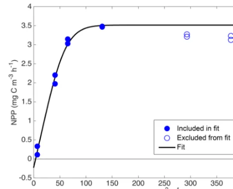
During the April and May cruises, daily 2 h 14C in-cubation experiments were conducted (n=28) to

esti-Figure 5.Example NPP vs. PAR relationship from14C incubations, with best-fit “PvE” curve.

mate photosynthetic parameters. Each day, a water sam-ple was taken from the Chl a maximum, as determined by in situ fluorescence, and duplicate 2 h 14C incubations were carried out at seven different PAR levels ranging from 0–400 µmol m−2s−1. The dark incubation 14C activ-ities were weakly but significantly correlated with Chl a (type-II linear regression; r2=0.19; p <0.05; apparent NPP=Chla·0.036±0.026 mg C mg Chla−1h−1+0.049±

0.035 mg C m−3h−1); dark activities were treated as sample-specific blanks and subtracted from the light incubation ac-tivities of the corresponding water sample. The resulting pro-ductivity estimates were interpreted as net primary produc-tivity (NPP) based on findings that most phytoplankton do not respire old carbon when newly fixed carbon is available (Marra and Barber, 2004; Pei and Laws, 2013). Note that if, contrary to our assumptions, phytoplankton did respire old carbon at all light levels during these incubations, then our calculations below overestimate NPP and underestimate phytoplankton respiration (R8), but GPP is unbiased. On the other hand, if old carbon is respired only in the low light in-cubations, then we underestimateR8and GPP, but little bias is introduced in NPP. Seven of the 350 individual NPP esti-mates (all from the April cruise) were judged to be positive outliers and were manually removed before further analy-sis. In∼60 % of the incubation experiments, NPP decreased with increasing PAR for PAR>200 µmol quanta m−2_s−1_.

We conclude that this apparent photoinhibition is likely not representative of most field conditions because in situ measurements of Chl a-normalized dO2/dt showed no

re-Chl

in situ (mg m

-3₎

0 2 4 6

PM

(mmol C m

-3 h -1) 0 2 4 6 8 10 12 14 16

y = 3.58±0.57x0.784±0.13

r2 = 0.88 RMSE = 1.32

(a)

Chl

in situ (mg m

-3₎

0 2 4 6

,

(mmol C m

-3 h -1 µmol -1 quanta m 2 s)

0 0.05 0.1 0.15 0.2 0.25

y = 0.0449±0.0051x0.813±0.092

r2 = 0.94 RMSE = 0.0118

(b)

Chl

in situ (mg m

-3₎

0 2 4 6

R?

(mmol C m

-3 h -1) -0.4 -0.2 0 0.2 0.4 0.6 0.8

y = 0.17±0.055x0.65±0.26

r2 = 0.64 RMSE = 0.0902

(c)

Data included in fit Data excluded from fit Least squares fit 95 % conf of fit

Figure 6.Photosynthetic parametersPm(a),α(b), andR8(c)vs. in situ Chlawith least squares power-law fits and 95 % confidence

intervals.R8estimates from April and June cruises are excluded from fit (panelc, open circles).

moved). Remaining NPP vs. PAR data were fit to an empiri-cal “PvE” model represented in Eqs. (6)–(8):

λ=PAR α Pm

ε, (6)

GPP=Pm 1+

1 ε

ε−1 X

i=0

e−λλ i

i!i−

ε−1 X

i=0

e−λλ i

i! !

, (7)

NPP=GPP−Rφ, (8)

based on four parameters: maximum GPP (Pm), the initial

slope of GPP/PAR (α), R8, and an efficiency factor (ε) representing the “sharpness” of the transition between light-limited and light-saturated photosynthesis. This parameter-ization is based on a conceptual model of photosynthesis in which there is a rate-limiting step that can receive and “store” up toε“packets” of energy at once at above the lim-iting rate without wasting any of these packets. We used a single ε value of 6, which provided the best overall least-squared fit across all incubation experiments. This ε value yields an NPP vs. PAR relationship that is “sharper” than the commonly used “tanh” model (Harrison and Platt, 1986) and more linear at low PAR, leading to smalleryoffset (smaller R8estimate). See Fig. 5 for example fits. A power law was then fit between in situ Chla estimates from the ship’s pro-filing package (calculated via Eq. 1) and each of the three parameters obtained from each NPP vs. PAR fit (Pm: Fig. 6a;

α: Fig. 6b; andR8: Fig. 6c). Fits withPm andαused data

from all cruises, but the fit withR8included only data from the process cruise (Fig. 6c; solid circles), as signals were too low to constrainR8in April andR8 appeared consistently higher during the June cruise, possibly due to higher temper-ature.

2.8.3 Chla-based GPP and NPP

The relationships in Fig. 6 were used to estimate photosyn-thetic parameters Pm(t, z), α(t, z), and R8(t, z) and their

uncertainty intervals at the float location from Chl a(t, z) (Sect. 2.3.5). We estimated gross primary productivity GPPChla(t, z) and net primary productivity NPPChla(t, z) via Eqs. (6)–(8) using the above photosynthetic parameters, PARextrapolated(t, z)(Sect. 2.6), andε=6 as input.

Uncertain-ties were propagated fromPm(t, z),α(t, z), andR8(t, z)

us-ing the conservative assumption that they covary (i.e., upper bound of NPPChlawas derived from upper bounds ofPmand

αand lower bound ofR8).

2.9 Area-weighted mean particle diameter

The area-weighted mean particle diameter Dbbp 10–50 m

depth bin was estimated following Briggs et al. (2013) via Eqs. (9)–(11):

Dbbp=2 s

Varbbp(t )

E

bbp(t )

V Qbb

1 γ (τ )

1

π, (9)

γ (τ )=

1−(3τ )−1 if τ ≥1

τ−τ2/3, if τ ≤1, (10)

τ= _t res tsamp , (11)

where Var[bbp(t )] is the variance inbbp due to the random

distribution of particles in space,E[bbp(t )]is meanbbp,V is

sensor sample volume,Qbb is the backscattering efficiency,

andγandτ are functions of residence time in the sample vol-umetres and sample integration timetsamp. Var[bbp(t )] and

E[bbp(t )]were calculated once per profile (ascent or descent)

using all data between 10 and 50 m. Prior to calculation of Var[bbp(t )], thebbptime series was de-trended by

Figure 7.Float patch mixed-layer time series of NO3(a), SiO4(a),

MLD(b), Chla(b), POCcp(c), O2(d), and the concentration of

O₂saturation(d).

(based on an empirical bbp/cp ratio of∼0.01 and

theoreti-cal value ofQc=2 for diameterwavelength; Bohren and

Huffman, 1983). Atresof 0.02 s was chosen based on a 6 mm

path through the sample volume and a platform velocity of 30 cm s−1, andtsampwas 1 s.

2.10 Sinking POC flux

POCbbp profiles from both gliders and the float were

di-vided into a “small” particle baseline (7-point running mini-mum followed by running maximini-mum) and a “large” particle “spike” signal (residuals above the baseline). This approach, developed by Briggs et al. (2011), is based on the finding that large, fast-sinking particles, owing to their rarity and light-scattering characteristics, can create individual large spikes in mesopelagicbbpclearly distinguishable from background

concentrations (Briggs et al., 2011). Large particle POCbbp

was multiplied by a bulk sinking speed of 75 m day−1to esti-mate large POC flux (Briggs et al., 2011). A broad plausible range of bulk sinking speeds 5±5 m day−1was used to esti-mate small POC sinking flux, which was added to large POC flux to yield total sinking POC flux. Sinking POC flux was bin averaged in 50 m vertical bins and either running 2-day bins (gliders) or longer discrete bins to match bloom stages (float).

Figure 8. Primary productivity estimates within the daily

mini-mum ML. GPPChla, GOP, GPPcp, and GPP from Bagniewski et

al. (2011), along with ML Chla. Diel-cycle-based estimates are

3-day means; other productivity estimates are daily, and Chlais

continuous.

3 Results

3.1 Evolution of the spring bloom

From float deployment through 17 April, MLD was vari-able (often>200 m but occasionally<50 m; Fig. 3), mixed-layer nutrients were high (NO3≈12 mmol m−3; SiO4≈

4 mmol m−3_{), biomass was low (Chl a≈0.35 mg m}−3_;

POCcp≈35 mg m−3), and O2 was undersaturated by

∼10 mmol m−3 (Fig. 7). Mixed-layer biomass concentra-tions increased over the next month, peaking in mid-May. This broad increase was punctuated by several 1–2-day pe-riods of decrease, most associated with clear mixed-layer deepening (Fig. 7). SiO4 was depleted to its lowest level

on 11 May, Chl a concentration peaked on 12 May, and NO3depletion and POCcpand O2concentrations peaked on

13 May. From bloom peak to 16 May, Chla decreased dra-matically (77 %), POCcp and O2 decreased moderately (by

9 and 13 mmol m−3, respectively), and NO3and SiO4

con-centrations recovered slightly (by 0.8 and 0.4 mmol m−3, re-spectively).

3.2 Primary productivity estimates

All GPP and GOP estimates were averaged into 3-day bins to improve the precision of the diel-cycle-based es-timates. To first order, GPPChla followed Chla by being low in early April (0.5–1.0 mmol m−3_day−1_{), peaking near}

Figure 9.Relationships between primary productivity estimates: GOP vs. GPPcp(a), GOP vs. GPPChla(b), GPPcpvs. GPPChla(c), and

GPPbbpvs. GPPChla(d). Type-I linear regressions are forced through the origin and include all data except the SiO4-depleted period (pink

circles). The expected range of GOP/GPP (a, b; dashed lines) assumes a photosynthetic quotient between 1–1.45 and 22–40 % of fixed

carbon released as DOC (see text).

9 May, GPPChla was strongly correlated with both cycle-based estimates of both GOP (Figs. 8 and 9b; blue) and GPPcp(Figs. 8 and 9c; blue). GOP was a factor of 2.1 higher

than GPPChla on a molar basis, while GPPcp was slightly

lower (factor of 0.81). GPPbbp was poorly correlated with

GPPChla and significantly lower (by 60 %; Fig. 9d). From noon 10 May to noon 11 May, diel cycles could not be calculated because the float was trapped at the surface due to high stratification and slight positive buoyancy. At peak biomass (11–13 May), and the bloom decline (13–16 May), both GOP/GPPChla and GPPcp/GPPChla were substan-tially lower than during bloom growth (Fig. 8, pink high-lighted region, and Fig. 9, pink symbols). In the post-bloom period (16–24 May), GOP/GPPChla and GPPcp/GPPChla increased again, similar to the bloom growth ratios (Figs. 8 and 9; red symbols). When all bloom phases are combined, best-fit ratios of GOP and GPPcpto GPPChlaare 1.7 and 0.6, respectively, and correlations are considerably less strong (r2 of 0.67 and 0.49, respectively). However, the estimates of productivity from diel cycles (GOP and GPPcp) remained

strongly correlated for the entire deployment. Over the en-tire study period, morning estimates of GOP and GPPcpwere

not significantly different from the afternoon estimates, while

morning GPPbbpestimates were significantly lower than

af-ternoon estimates (80 % lower overall). However, morning– afternoon patterns appear to change starting on 13 May, when the bloom decline starts (e.g., Fig. 4). From 13–24 May, there is no significant difference between morning and af-ternoon GPPbbp, but afternoon estimates of GPPcpand GOP

were lower than morning estimates by 70 and 43 %, respec-tively. These differences were near the threshold of statistical significance: mean afternoon–morning difference ±2 stan-dard errors was−2.3±2.3 mmol m−3day−1for GPPcp and

−3.0±2.5 mmol m−3day−1for GOP.

3.3 Depth integrated GPP, NPP, and NCP and carbon export

Figure 10.Estimates of sources and sinks of organic carbon

inte-grated over the top 60 m: GPPChlaand NPPChlaand sinking

par-ticle export (this study), as well as NCP and loss due to the sum of sinking particle export and net DOC production and sinking parti-cle export only (Alkire et al., 2012). Bloom periods follow Alkire et al. (2012) and are defined in the text (Sect. 3.3).

Each budget term carries considerable uncertainty, but based on the central estimates, the partitioning of fixed carbon ap-peared to change substantially over the course of the bloom. Note that these NCP estimates include the net production of dissolved organic carbon (DOC), while NPPChla excludes any photosynthetic DOC production. NPPChlaand NCP es-timates were similar during the early and main bloom, sug-gesting moderate to low heterotrophic respiration. During the early bloom period, export was also low (∼22–28 % of GPPChla), allowing for the rapid accumulation of biomass. During the main bloom, GPPChlanearly doubled as biomass increased, but a larger fraction (∼50 %) was exported, leav-ing∼25 % to accumulate. During the bloom decline, appar-ent community respiration (defined as the difference between GPPChla and NCP) was 156 % of GPPChlaand export was an additional 50–80 %. In the post-bloom period, community respiration was again high (∼100 % of GPP), and export was much lower (0–15 % of GPP). Our NPPChla estimates and bbpspike-based sinking flux estimates provide a continuous,

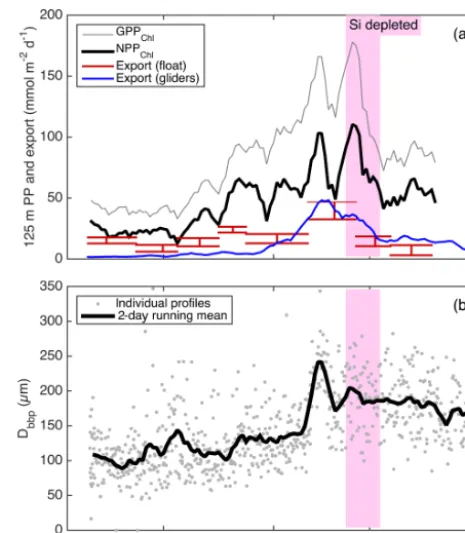
high-resolution picture of the link between productivity and export at 125 m for the entire study period (Fig. 11a). Float-and glider-based POC export estimates agree broadly at this depth (red lines), suggesting that the higher-resolution glider time series are representative of the float patch as well. While export at 125 m is coupled with NPPChla(Fig. 11a), there is a rapid increase in export efficiency between 3 and 6 May from ∼20 to 40 %. Area-weighted mean particle diameter (Dbbp) ranged from 90–150 µm during April and peaked at

250 µm on 7–8 May (Fig. 11b), coincident with peak biomass as measured by both Chlaand POCbbpfrom the gliders (not

shown).Dbbpfell rapidly on 9 May, coincident with an ML

Figure 11. (a)Continuous productivity and export from the au-tonomous float and gliders to and from the top 125 m over the en-tire study period. Productivity and glider export are 2-day running means, while float export is averaged over longer periods denoted by the width of the bars. Bar height denotes uncertainty bounds.

(b)Near-surface gliderDbbpestimates from 10–50 m.

deepening event. Post-bloomDbbpranged from 150–190 µm

(Fig. 11b).

4 Discussion

4.1 Accuracy of PP estimates

The combination of three estimates of primary productivity and one estimate of community productivity, all from the same platform at comparable temporal and horizontal scales, provides a unique opportunity to evaluate the accuracy of all methods. Each of our PP methods is discussed in turn in Sect. 4.1.1–4.1.4.

4.1.1 GPPChla

GPPChla and GPPcpare estimates of the same quantity

ob-tained independently. GPPChla is derived from PAR and Chl a estimates using robust local parameterizations ob-tained from14C incubations. GPPcpis derived entirely from

cpmeasurements converted to POC using another robust,

lo-cal conditions (Bagniewski et al., 2011). In this context, the combination of strong correlation and absolute agreement between GPPChla and GPPcp (Fig. 9c; within 19 %)

pro-vides confidence in both methods during the bloom growth and post-bloom periods. The GOP/GPPChla slope of 2.1 (Fig. 9b) is at the upper end of the expected range, pro-viding additional first-order support for GPPChla accuracy. Neither GPP method includes DOC production, so the range of expected photosynthetic quotients (∼1–1.45; Laws, 1991; Robertson et al., 1993), combined with the fraction of GPP released as DOC in marine and estuarine environments (2– 50 %; Baines and Pace, 1991), implies a possible GOP/GPP range of 1–2.9. During the main bloom observed by the float in this study, Alkire et al. (2012) estimate that DOC accounts for 22–40 % of NCP in the mixed layer. If these estimates apply to GPP as well, our expected GOP/GPP range nar-rows to 1.3–2.4 (Fig. 9a, b; gray dashed lines). Thus, our GOP estimates suggest either that both the photosynthetic quotient and phytoplankton DOC production are high dur-ing bloom growth (and GPP is accurate) or that both GPP estimates are biased low. As mentioned in Sect. 2.8.2, a neg-ative bias in GPPmodel could be explained if phytoplankton

respired substantial old, unlabeled carbon in our low light in-cubations, but not in the high light incubations. In this case a separate explanation (see next section) is needed for the high GOP/GPPcpslope of 2.6 (Fig. 9a).

During bloom peak and decline, the strong discrepancies between GPPcpand GPPChlaimply either an underestimate by GPPcp (discussed in the next section) or an

overesti-mate by GPPChla. If diatoms reduce GPP in response to

sustained SiO4 limitation, then we expect GPPChla over-estimation at peak biomass given that GPPChla is only a function of Chla and PAR, without any nutrient limitation term. Twelve mixed-layer SiO4samples were collected in the

vicinity of the float on 11–13 May, and the mean and max-imum measured concentrations were 0.3 and 0.6 mmol m−3, respectively, suggesting that diatom growth was most likely severely limited (Fig. 7a). This does not necessarily imply that diatom carbon fixation rates were reduced, but previ-ous studies have indeed observed a large and reversible re-duction in apparent diatom photosynthetic efficiency under multi-day SiO4 limitation (Lippemeier et al., 1999, 2001).

Both FlowCAM microscopy and HPLC pigments indicate that diatoms accounted for≥50 % of phytoplankton biomass at bloom peak (Cetini´c et al., 2015), so we expect a substan-tial reduction in bulk phytoplankton growth (and likely GPP) under these conditions. This expectation, combined with the observed reduction in both GPPcpand GOP at bloom peak,

leads us to conclude that GPPChla is most likely overesti-mated at bloom peak. This conclusion agrees with the cou-pled physical–biological model of Bagniewski et al. (2011), which assimilated float biogeochemical measurements and achieved optimal fit when diatom GPP was limited by SiO4

with a half-saturation constant of 1 µmol m−3. GPP inferred from this model closely matches our observed GPPcp

dur-ing SiO4limitation (Fig. 8, gray line vs. black circles), even

though Bagniewski et al. (2011) assimilated daily binned data, removing any diel cycle information. On the other hand, three14C incubations were conducted between 10 and 14 May using water with SiO4<0.5 mmol m−3, although not

at the float location, and there was not a substantial reduction in measuredPm. These samples may not be representative of

the water sampled by the float, despite similar Chlaand SiO4

concentrations, or it is possible that a bottle effect enhanced GPP. But we cannot rule out the alternative hypothesis that the Si-limited community continued to fix carbon at a con-stant rate and that GPPcp and GOP estimates were reduced

for another reason (discussed in next sections).

Apart from Si limitation, possible explanations for GPPChlaoverestimation include overestimation of Chladue to increased fluorescence, underestimation of the MLD, or photoinhibition. Again, Chla was calculated the same way for the floats and ship, so if the in situ fluorometric method overestimated Chla at bloom peak, we would expect to see a deviation from the observed relationships between photo-synthetic parameters and Chla(Fig. 6). So this explanation, while plausible given the high Chl a / bbp ratio at bloom

peak (Cetini´c et al., 2015), also requires that none of our low SiO4 bottle samples were representative of the bloom

peak at the float location. The density-based MLD estimates appear quite robust during this period, consistently shallow and stable at 10–20 m and matched by the vertical motion of the float. And the daytime increases in O2 (Fig. 4) andcp

on 11 and 12 May show no sign of photoinhibition, despite a peak hourly-averaged PAR of>750 µmol m−2s−1; increases are smooth throughout the morning and appear to continue at the same rate in the afternoon (Fig. 4). This result sup-ports our decision to exclude photoinhibited bottle incuba-tion data from our productivity vs. PAR fits, and we suggest that photoinhibition terms from bottle incubations should be applied with caution, if at all, in future studies. In this sys-tem, photoinhibition is likely reduced during deeper mixing events due to the shorter time phytoplankton is exposed to high light. During the stratified conditions, reduction in pho-toinhibition can be attributed to photoadaptation.

SiO4limitation may also explain some of the discrepancy

between GPPcpand GPPChladuring the bloom decline (13– 16 May), at least when afternoon estimates are excluded (see Fig. 9b, c; open pink circles). Lower afternoon GPPcp and

GOP, combined with very shallow (<5 m) MLDs at noon on 13 and 15 May, also raise the possibility of significant photo-damage inhibiting afternoon productivity. Mean ML PAR ex-ceeded 500 µmol m−2_s−1_{for at least 2 h on both days.}

How-ever, the negative afternoon GPPcpestimates at this time

sug-gest a bias in the diel cycle method as well (see next section). 4.1.2 GPPcp

Potential sources of bias unique to GPPcpinclude a diel cycle

cycle in export loss, or a diel cycle in the POC/ cpratio. The

tight correlations between GPPcp and GOP throughout the

entire study period (r2=0.95; Fig. 9a) and between GPPcp

and GPPChladuring bloom growth (r2=0.96; Fig. 9b) pro-vide encouraging support for GPPcpas a measure of relative

primary productivity at the very least. Furthermore, the quan-titative agreement between GPPcpand GPPChladuring both bloom growth and post-bloom (Fig. 9c; slope: 0.82±0.06) is very close to our expected slope of 0.93 from model re-sults (reanalysis of Bagniewski et al., 2011), suggesting that GPPcpaccuracy is comparable to other methods across most

of the conditions encountered. These findings agree closely with those of White et al. (2017), who find a GPPcp/NPP

ratio of 1.1 across a factor of 3 dynamic range of productiv-ities in the subtropical North Pacific, suggesting that GPPcp

is either accurate or slightly underestimates true GPP. Taken together, our results are highly encouraging regarding the widespread applicability and accuracy of the GPPcpmethod.

However, it should be noted that our results still may not ap-ply to certain other systems in which different phytoplank-ton size and/or timing of cell division could alter the diel POC/ cprelationship (Dall’Olmo et al., 2011).

If the SiO4 limitation hypothesis is correct, then GPPcp

during the bloom peak and morning GPPcpduring the bloom

decline may be accurate as well. On the other hand, if GPPChla is accurate during this time, then GPPcpis biased

low by ∼50 % at this time. It is unclear what might cause such a low bias, especially at bloom peak. Between the af-ternoon of 11 May and the morning of 13 May, there is no anomaly in the diel cycles of POCcp or O2 (Fig. 10)

in-dicative of daytime mixing, advection, or possible photoin-hibition, and there is no change in the relationship between GPPcpand GOP (Fig. 9a; rightmost pink symbol). Without

grazing data, we cannot rule out enhanced daytime grazing as a possible explanation, although grazing is generally ex-pected to be higher at night. Alternatively, particularly high photooxidation could potentially dampen O2diel cycles

dur-ing this period and perhaps cp diel cycles as well. This

hy-pothesis is supported by laboratory measurements of diatom productivity under nutrient limitation (Spilling et al., 2015), although again we would need to explain why reduced Pm

was not observed in our bottle incubations. On the other hand, the afternoon GPPcp estimates during the bloom

de-cline period show a clear example of negative bias in the diel cycle method. On 13, 14, and 15 May (bloom decline), the rates of net POCcp(and O2) accumulation are positive or near

zero in the morning but negative each afternoon (e.g., Fig. 4; 13 May). One plausible explanation is horizontal advection of the float relative to the ML during its afternoon profile, causing it to resurface in water with lower biomass. During this period, comparison with ship, autonomous glider, and satellite measurements (Alkire et al., 2012) shows that the float was at the edge of a high biomass (and O2) patch, so

advection during this time would most likely cause a loss in POCcpand O2. Note that the afternoon reductions in GPPcp

during bloom decline are greater than the afternoon reduc-tions in GOP (e.g., Fig. 4). This result is possible with the horizontal advection and mixing hypothesis alone, but high export combined with a shallow afternoon MLD may also play a role. Shallow MLD enhances the loss of ML concen-tration for a given export rate, and nighttime mixing can re-entrain some of this export, reducing the ML POC diel cycle relative to the O2diel cycle.

4.1.3 GOP

The tight fit between GOP and both GPP estimates over most of the study period provides important support for the O2

diel cycle method as a measure of relative primary produc-tion in this region. Again, because all estimates were in-dependent and taken at the same scale, and because the 2-month deployment allowed 14 independent matchups at a 3-day timescale spanning a wide range of productivities, this dataset represents the most extensive validation to date of the O2 diel cycle method as a measure of relative primary

pro-ductivity. Additionally, the overall accuracy of our GOP es-timates may be assessed indirectly through comparison with independent ship-based GOP estimates made during the May process cruise (Quay et al., 2012) and through comparison of our GOP/GPP and GOP/NPP ratio estimates with pre-vious estimates from this region. Quay et al. (2012) esti-mated ML-integrated GOP using measurements of three oxy-gen isotopes,16O,17O, and18O, taken daily between 3 and 21 May during the process cruise. Mean GOP calculated by this method was 245 mmol O2m−2day−1. This method

inte-grates over several weeks, so we interpret their estimate to correspond roughly to mean ML depth-integrated GOP be-tween 19 April (2 weeks before the first sample) and 21 May. For comparison, we multiply each half-day GOP estimate by MLD to obtain ML-integrated GOP and obtain an aver-age from 19 April to 21 May of 149 mmol m−2day−1, 40 % lower than the Quay et al. (2012) estimate. However, our es-timate integrates to the daily minimum MLD, and while the triple O2isotope method assumes constant MLD, we expect

it to more closely approximate daily maximum MLD in the presence of diel MLD fluctuations given its long integration time. Mean GPPChladuring this period, integrated to the bot-tom of the dailyminimumMLD, is 30 % lower than mean GPPChla integrated to the daily maximumMLD. If we as-sume the same relative difference for GOP, we obtain a re-vised ML-integrated GOP estimate of 213 mmol m−2day−1, 13 % lower than the Quay et al. (2012) estimate. Given the uncertainties associated with the GOP methods and the dif-fering spatiotemporal scales, this result provides first-order support for the accuracy of both methods. Our findings re-inforce those of Hamme et al. (2012), who in the Southern Ocean in March–April found that mean ML-integrated GOP calculated via O2/Ar diel cycles (similar to our method) was

Bender et al. (1992) calculated a GOP/NPP ratio of 2.5 during the spring bloom in the northeast Atlantic us-ing in situ 18O incubations and 24 h 14C incubations. We calculate GOP/NPPChla as shown in Fig. 9b, but replace GPPChlawith NPPChlaand obtain a best-fit ratio and 95 % confidence interval of 2.4±0.2 for the bloom growth pe-riod and 1.7±0.4 for the entire deployment. These fits ap-pear to support the accuracy of both our NPPChlaand GOP estimates during the bloom growth phase, consistent with our other findings. However, our GOP/GPP ratio estimates of 2.6±0.2 (Fig. 9a) and 2.1±0.2 (Fig. 9b) are near or above the high end of our expected range of 1.3–2.4 (see Sect. 4.1.1). As discussed in previous sections, these ratios may be the result of a high photosynthetic quotient and high DOC production combined with a small negative bias in GPPcp. Our GOP estimates may also be too high, but we

can-not think of a plausible mechanism that would cause a sub-stantial overestimate of diel-based GOP (but not of GPPcp).

Regardless of the source of our high GOP/GPP ratios, they are also consistent with Hamme et al. (2012), who also es-timated GPP from on-deck PvE incubations and GOP via O2/Ar diel cycles, providing a very close methodological

comparison in a different environment (autumn, Southern Ocean). They obtain an even higher GOP/GPP ratio of 3.6. However, Hamme et al. (2012) assumed that 1–2 h 14C in-cubations represent GPP, while we assume that these same incubations represent NPP (when NPP>0). If our assump-tion is correct, then their method provides a quantity closer to daytime NPP than GPP. However, even in this case, assuming moderate daytime phytoplankton respiration rates (≤30 % of GPP), GOP/GPP during their study was >2.5, which is in agreement with our estimates. It is also worth noting that related studies comparing diel cycles in O2andpCO2

measurements (Johnson, 2010; Merlivat et al., 2015), both of which include the effects of DOC production, have found ratios of daytime oxygen production to carbon production that are within the expected range of 1–1.45. These results provide further support for diel-cycle-based O2 production

and the hypothesis that DOC production may drive the high GOP/GPP observed in this and other studies (Bender et al., 1992; Hamme et al., 2012).

In total, the available evidence provides first-order support for the accuracy of our diel-cycle-based GOP estimates. Our findings build on important recent work in diverse environ-ments showing that diel cycles in the O2/Ar ratio yield ML

GOP estimates that are consistent with independent GOP es-timates (Hamme et al., 2012) and that diel cycles in O2

mea-surements from autonomous gliders in the subtropical Pacific provide GOP estimates that are a reasonable multiple of in-dependent NPP results (Nicholson et al., 2015). Our results add a third ocean region (springtime North Atlantic) and a third platform (Lagrangian mixed-layer float) in addition to new comparisons withcpandbbpdiel cycles.

4.1.4 GPPbbp

Because diurnal variability inbbpcan be estimated from

geo-stationary satellites (Neukermans et al., 2012), the ability to accurately estimate GPP from bbp diel cycles would be

extremely valuable. While ship-based measurements from NAB08 show that bbp andcp were equally well correlated

with POC over the May cruise (Cetini´c et al., 2012), the poor matchups we find between GPPChlaand GPPbbpsuggest that

diel changes are present in POC/ bbp and can cause strong,

consistent bias in GPPbbp. Our results agree with previous

findings that while beam attenuation and forward scattering by phytoplankton increase immediately after they begin to photosynthesize,bbpand side scattering often do not, both in

the lab (Ackleson et al., 1993; Poulin et al., 2018) and in the ocean (Kheireddine and Antoine, 2014). These results cau-tion against the use ofbbpdiel cycles to estimate GPP without

further research. However, it is worth noting that our after-noon GPPbbp estimates are reasonably well correlated with

GPPChla(r2=0.63,m=0.75±0.23; data not shown) dur-ing the bloom growth period. If this result is found to be ro-bust in other times and places, then a useful estimate of GPP from satellite (and other)bbp time series may be possible.

However, even if thebbpdiel cycle cannot be used to estimate

GPP, it likely contains other useful information, especially in combination withcp and/or O2. If robust relationships

be-tween plankton communities and/or physiology andbbpdiel

cycles can be established (and, ideally, understood mecha-nistically), then measurements ofbbp diel cycles may still

provide valuable oceanographic information, whether from in situ platforms or satellites.

4.2 Combined upper layer carbon budgets

Taken together with the Alkire et al. (2012) NCP and car-bon export estimates and our adaptation of the Briggs et al. (2011) depth-resolved carbon fluxes, our productivity and bulk particle estimates provide a remarkably detailed, high-resolution picture of carbon flows over the entire spring bloom. From 4–17 April, ML Chla, POC, and O2

concentra-tions changed little despite large fluctuaconcentra-tions in MLD, while NO3increased slightly during deep mixing, presumably due

to entrainment, but was stable during shallow (<100 m) mix-ing. Consistent positive 125 m integrated NPPChla(Fig. 11a) was therefore likely balanced by heterotrophic respiration. From 18 April to 7 May, ML shoaling events coincided with several pulses of high net growth in POCcpand Chla

of fragile aggregates containing live phytoplankton including

Chaetoceros sp. resting spores (Martin et al., 2011; Briggs et al., 2011; Rynearson et al., 2013). This aggregate ex-port was the largest loss term of surface POC during the “main bloom”, reducing the biomass accumulation rate by

≥50 % (Fig. 10). While SiO4 limitation has been proposed

as a cause of this rapid sinking event (Bagniewski et al., 2011), this aggregation commenced when SiO4

concentra-tions were still>2 mmol m−3(Fig. 7a) and 5 days prior to the ∼35 % reduction in GOP and GPPcp that we attribute

to SiO4limitation (pink band in Fig. 11b). The exact cause

of this rapid aggregation event is unknown, but likely in-volves a combination of moderately high particle concentra-tion (POCcp>10 mmol m−3), weakening of mixing (which

could break fragile aggregates), and production of transpar-ent exopolymer particles (Martin et al., 2011; Alkire et al., 2012). The combination of high export and reduced produc-tivity at the end of the diatom bloom (12–14 May) appears to end the ML biomass accumulation. However, we con-clude that the subsequent sharp decline in ML Chla, POCcp,

and O2 from 14–15 May (Fig. 7) was probably not the

re-sult of a dramatic increase in heterotrophic respiration, as implied by the strong negative NCP estimate (Fig. 10) of Alkire et al. (2012). Our conclusion stems from the night-time ML O2loss rates, which do not increase at all between

the bloom peak the bloom decline (see Fig. 4a). Instead, the ML O2 decline appears to be caused by further GPP

de-creases due to continued SiO4 limitation and a decline in

Chla (Fig. 7b, d), likely enhanced by the export of phyto-plankton from the shallow ML. The O2decline (and

accel-erating Chl a decline) may have been enhanced by the ad-vection of the float relative to the thin surface ML during afternoon profiles (see Sect. 4.1.2), or perhaps an additional light-dependent process, such as photoinhibition or photores-piration (Spilling et al., 2015), nearly eliminated GPP dur-ing this time, but only in the afternoons. After the decline of the diatom bloom, the different productivity estimates again provide a consistent picture, this time of top-down control. GOP and GPPcp again show no sign of nutrient limitation

(Fig. 9b, c, red symbols), and NPPChla is apparently bal-anced by heterotrophic respiration. Glider estimates of sink-ing POC export were low, but higher than early bloom export, despite similar NPP (Fig. 11a) and higher respiration. This result highlights the decoupling between NCP and export on weekly to monthly timescales in this dynamic system and suggests that biomass and particle size are better predictors of sub-seasonal export dynamics. The changing export effi-ciencies that we observed (<15 % through most of April, to

∼57 % during the main bloom, to∼33 % in the post-bloom period) provide a complex picture of “the spring bloom”, but still agree broadly with the export ratio of 45 % calculated by Buesseler and Boyd (2009) in the North Atlantic spring bloom using JGOFS data, which is among the highest ex-port efficiencies observed in the open ocean. However, unlike Buesseler and Boyd (2009) and in line with the conclusions

of Martin et al. (1993), we see significant flux attenuation in the 100 m below the euphotic zone. For example, 35–48 % of flux is lost between 60 m (Fig. 10) and 125 m (Fig. 11a) during the main bloom.

5 Conclusions

Our results, placed in the context of previous studies, pro-vide strong support for the diel cycle method as a means to obtain estimates of GOP (from O2) and GPP (fromcp) with

reasonable accuracy relative to existing methods and enough precision on 3-day timescales to clearly resolve a spring di-atom bloom. The range of biomass, mixing regimes, and phy-toplankton communities in this study, combined with previ-ous results from the subtropics, suggest that these methods are not overly dependent on particular ocean conditions. Be-cause the diel cycle method is well suited for autonomous platforms, it has the potential to greatly increase our cov-erage of in situ productivity estimates, providing both di-rect knowledge of this critical biological rate and greatly enhanced validation datasets for satellite-derived and mod-eled productivity. Our results also support the use of short-term14C incubations to parameterize simple PvE models for application to autonomous measurements, at least in the ab-sence of strong nutrient limitation. We find high GOP/GPP ratios of 2.1–2.6 through most of the study, suggesting high DOC production and/or a possible moderate underestimation of GPP by both methods. Finally, combined high-resolution estimates of NPP, particle size, and sinking flux during the North Atlantic spring bloom show strong coupling between the three, modulated by a dramatic increase in export effi-ciency at bloom peak, apparently due to rapid aggregation.

Appendix A: Abbreviations used in more than one subsection of the text

bbp Particulate optical backscattering coefficient

Chla Chlorophyllaconcentration

cp Particulate optical beam attenuation coefficient

Dbbp Area-weighted mean particle diameter from optical backscattering

DOC Dissolved organic carbon concentration GOP Gross O2productivity from O2diel cycles

GPP Gross primary productivity

GPPbbp GPP from optical backscattering diel cycles

GPPChla GPP from in situ chlorophyll and light measurements GPPcp GPP from optical beam attenuation diel cycles

JGOFS Joint Global Ocean Flux Study KPAR Diffuse attenuation coefficient of PAR

ML Mixed layer

MLD Mixed-layer depth NPP Net primary productivity

NPPChla NPP from in situ chlorophyll and light measurements PAR Photosynthetically available radiation

Pm Maximum GPP (light saturated)

POC Particulate organic carbon concentration POCbbp POC from optical backscattering

POCcp POC from optical beam attenuation

PP Primary productivity

R8 Phytoplankton respiration rate

S Salinity

T Temperature

α Initial slope GPP/PAR (light limited)

Competing interests. The authors declare that they have no conflict of interest.

Acknowledgements. The collection of data for this study was funded by the US National Science Foundation (grants OCE-0628107 and OCE-0628379) and NASA (grants NNX-08AL92G and NNX-10AP29H). Analysis and writing was further funded by a University of Maine Doctoral Research Fellowship, Na-tional Science Foundation grant OCE-1420929, and a European Research Council grant. The authors would also like to thank Andrew Thomas and Emmanuel Boss for valuable comments and feedback as PhD committee members and the crew and technicians

of the RV Knorr and RV Bjarni Saemundsson for making this

entire study possible. We would also like to thank two anonymous reviewers for their feedback, which has substantially improved this paper.

Edited by: Gerhard Herndl

Reviewed by: two anonymous referees

References

Ackleson, S. G., Cullen, J. J., Brown, J., and Lesser, M.: Irradiance-Induced Variability in Light Scatter from Marine Phytoplankton in Culture, J. Plankton Res., 15, 737–759, 1993.

Alkire, M. B., D’Asaro, E., Lee, C., Perry, M. J., Gray, A., Cetini´c, I., Briggs, N., Rehm, E., Kallin, E., Kaiser, J., and González-Posada, A.: Estimates of Net Community Production and

Ex-port Using High-Resolution, Lagrangian Measurements of O2,

NO−₃, and POC through the Evolution of a Spring Diatom

Bloom in the North Atlantic, Deep-Sea Res. Pt. I, 64, 157–174, https://doi.org/10.1016/j.dsr.2012.01.012, 2012.

Bagniewski, W., Fennel, K., Perry, M. J., and D’Asaro, E. A.: Op-timizing models of the North Atlantic spring bloom using phys-ical, chemical and bio-optical observations from a Lagrangian float, Biogeosciences, 8, 1291–1307, https://doi.org/10.5194/bg-8-1291-2011, 2011.

Baines, S. B. and Pace, M. L.: The Production of Dissolved Organic Matter by Phytoplankton and Its Importance to Bacteria: Petterns across Marine and Freshwater Systems, Limnol. Oceanogr., 36, 1078–1090, https://doi.org/10.4319/lo.1991.36.6.1078, 1991. Bender, M., Ducklow, H., Kiddon, J., Marra, J., and Martin, J.: The

Carbon Balance during the 1989 Spring Bloom in the North

At-lantic Ocean, 47◦N, 20◦W, Deep-Sea Res. Pt. I, 39, 1707–1725,

1992.

Bohren, C. F. and Huffman, D. R.: Absorption and Scattering of Light by Small Particles, John Wiley & Sons, New York, 1983. Briggs, N., Perry, M. J., Cetini´c, I., Lee, C., D’Asaro, E.,

Gray, A. M., and Rehm, E.: High-Resolution Observa-tions of Aggregate Flux during a Sub-Polar North At-lantic Spring Bloom, Deep-Sea Res. Pt. I, 58, 1031–1039, https://doi.org/10.1016/j.dsr.2011.07.007, 2011.

Briggs, N. T., Slade, W. H., Boss, E., and Perry, M. J.: Method for Estimating Mean Particle Size from High-Frequency Fluc-tuations in Beam Attenuation or Scattering Measurements, Appl. Optics, 52, 6710–6725, 2013.

Buesseler, K. O. and Boyd, P. W.: Shedding Light on Processes That Control Particle Export and Flux Attenuation in the Twi-light Zone of the Open Ocean, Limnol. Oceanogr., 54, 1210– 1232, 2009.

Caffrey, J. M.: Production, Respiration and Net Ecosystem Metabolism in U.S. Estuaries, in: Coastal Monitoring through Partnerships, edited by: Melzian, B. D., Engle, V., McAlister, M., Sandhu, S., and Eads, L. K., Springer, Springer Science and Business Media, Dordrecht, the Netherlands, 81, 207–219, https://doi.org/10.1007/978-94-017-0299-7_19, 2003.

Cetini´c, I., Perry, M. J., Briggs, N. T., Kallin, E., D’Asaro, E. A., and Lee, C. M.: Particulate Organic Carbon and Inherent Optical Properties during 2008 North Atlantic

Bloom Experiment, J. Geophys. Res., 117, C06028,

https://doi.org/10.1029/2011JC007771, 2012.

Cetini´c, I., Perry, M. J., D’Asaro, E., Briggs, N., Poulton, N., Sier-acki, M. E., and Lee, C. M.: A simple optical index shows spatial and temporal heterogeneity in phytoplankton community composition during the 2008 North Atlantic Bloom Experiment, Biogeosciences, 12, 2179–2194, https://doi.org/10.5194/bg-12-2179-2015, 2015.

Claustre, H., Morel, A., Babin, M., Cailliau, C., Marie, D., Marty, J. C., Tailliez, D., and Vaulot, D.: Variability in Particle Attenuation and Chlorophyll Fluorescence in the Tropical Pacific: Scales, Patterns, and Biogeochemical Implications, J. Geophys. Res.-Oceans, 104, 3401–3422, https://doi.org/10.1029/98jc01334, 1999.

Cullen, J. J., Lewis, M. R., Davis, C. O., and Barber, R. T.: Photosynthetic Characteristics and Estimated Growth Rates In-dicate Grazing Is the Proximate Control of Primary Produc-tion in the Equatorial Pacific, J. Geophys. Res., 97, 639, https://doi.org/10.1029/91JC01320, 1992.

Dall’Olmo, G., Boss, E., Behrenfeld, M. J., Westberry, T. K., Courties, C., Prieur, L., Pujo-Pay, M., Hardman-Mountford, N., and Moutin, T.: Inferring phytoplankton carbon and eco-physiological rates from diel cycles of spectral particulate beam-attenuation coefficient, Biogeosciences, 8, 3423–3439, https://doi.org/10.5194/bg-8-3423-2011, 2011.

D’Asaro, E. A.: Performance of Autonomous Lagrangian Floats, J. Atmos. Ocean. Tech., 20, 896–911, 2003.

D’Asaro, E., Lee, C., and Perry, M. J.: Data from the North Atlantic Bloom 2008 project, Biological and Chemical Oceanography Data Management Office (BCO-DMO), https://www.bco-dmo. org/project/2098, last access: 24 July 2018.

García, H. E. and Gordon, L. I.: Oxygen Solubility in Seawa-ter: Better Fitting Equations, Limnol. Oceanogr., 1307–1312, https://doi.org/10.4319/lo.1992.37.6.1307, 1992.

Gernez, P., Antoine, D., and Huot, Y.: Diel Cycles of the Par-ticulate Beam Attenuation Coefficient under Varying Trophic Conditions in the Northwestern Mediterranean Sea: Ob-servations and Modeling, Limnol. Oceanogr., 56, 17–36, https://doi.org/10.4319/lo.2011.56.1.0017, 2011.

Hamme, R. C., Cassar, N., Lance, V. P., Vaillancourt, R. D., Bender, M. L., Strutton, P. G., Moore, T. S., DeGrandpre, M. D., Sabine,

C. L., Ho, D. T., and Hargreaves, B. R.: Dissolved O2/Ar and