Gender differences in commute time and pay

(1)

Next release: To be announced Release date:

4 September 2019 Contact:

Vahé Nafilyan

[email protected] +44 (0)1633 455046

Article

Gender differences in commute time and pay

A study into the gender gap for pay and commuting time, using data from the Annual

Survey of Hours and Earnings.

1 . Introduction

The gender pay gap, defined as the difference in median pay between men and women, has received growing attention from researchers, policy makers and the wider public. The gender pay gap has been falling in the last two decades but remains substantial: full-time employed women earned 8.6% less than full-time employed men in 2018, down from 17.4% in 1998 (see Gender pay gap in the UK: 2018).

Understanding the causes of the gender pay gap is crucial to provide adequate policy recommendations to close the gender pay gap. The gender pay gap can no longer be explained by differences in educational attainment, as women now have better educational attainment than men. However, the gender pay gap is not necessarily because of discrimination by employers. Other explanations have been proposed in the literature. Differences in psychological attributes, such as attitudes towards risk, competition and negotiation, are well documented (Bertrand, 2011) but only explain a small fraction of the gender pay gap (Blau and Kahn, 2017; Bertrand, 2018). Recent evidence highlights that family and fertility decisions may be an important driver of the gender pay gap. Having children typically leads to career interruption for women but not men, which may explain some of the gender pay gap (Costa-Dias et al., 2018; Kleven et al., 2019). In addition, the difficulty for women to combine work and family, especially to work long or particular hours, could further explain the gender pay gap (Goldin, 2014). Some evidence from the US suggests that women tend to favour jobs with greater flexibility and fewer hours, at the expense of pay (Mas and Pallais, 2017; Wiswall and Zafar, 2018).

These studies highlight that measuring gender differences in job attributes other than wages is important to understand the causes of the gender pay gap. Using data from the Annual Survey of Hours and Earnings (ASHE), in this study we document the gender differences in commuting time. First, we highlight that the commuting gap follows the same age pattern as the gender pay gap. Second, we investigate whether women favour jobs with shorter commutes, at the expense of pay. To do so, we examine whether the reasons for job separation differ between men and women. We find that commuting time has a greater impact on the decision to leave one’s job for women than men. By contrast, hourly rate has a greater impact on men than on women. If the gender pay gap is partly caused by women’s willingness to accept lower wages in exchange for greater flexibility and shorter commutes, then closing the gender pay gap would involve addressing the reasons why women favour more flexible jobs.

In the first section, we present the data we use for this analysis: we describe the methodology used to estimate commuting time in ASHE based on postcode information. In the second section, we provide some descriptive evidence, showing gender differences in pay and commuting time. In the third section, we examine whether the motivations for changing job differ between men and women, and we outline the methodology and present the results. The last section concludes the analysis.

2 . Data

The Annual Survey of Hours and Earnings (ASHE) provides information about the levels, distribution and make-up of earnings and hours paid for employees in the UK. The ASHE is based on a 1% sample of employee jobs taken from HM Revenue and Customs Pay As You Earn (PAYE) records. The ASHE is used for key labour market indicators such as average weekly earnings.

ASHE does not provide direct information on commuting time or mode. However, it contains information on the postcode of the home and workplace of the employee. We use these postcodes to estimate commuting time from home to work using a trip planner app. (See Appendix for more detail on how we derived the commuting times, and how they compare with self-reported commuting times from other surveys.) The commuting time measures the time it takes to travel from the postcode of the employee to the postcode of the employer.

(3)

We restrict our sample to working age adults (aged 16 to 65 years) living in Great Britain (we exclude individuals living in Northern Ireland because no estimates of commuting time could be obtained for these respondents). We focus on individuals’ main job and remove records for second or third jobs. We removed the few records with missing data; with hourly pay higher or lower than the top or bottom 0.5% of the distribution; or where the reported hours worked are less than two.

In the second part of this paper, we test whether pay and commuting distance affect the decision to change job differently for men and women. We use the longitudinal dimension of the ASHE to identify those who leave their job between two waves. The ASHE only collects data for individuals who are in the PAYE system; therefore, all those who are not in employment or are self-employed in year t would not be included in the ASHE. However, not being in the dataset in year t does not necessarily imply that the individual is not employed. Some individuals may not appear in the ASHE but may nonetheless still be employed, because their employers did not fill in the survey in year t. To avoid identifying these individuals as job leavers, we do not classify as leavers those who are not in the ASHE in year t but are employed with the same employer in year t - 1 and t + 1 or t + 2. By doing so, we minimise the impact of missing data. Because of this approach, we only have reliable information about job leaver status from 2004 to 2016.

(4)

[image:4.595.262.538.56.531.2]

Table 1: Summary statistics

All Men Women

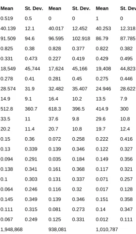
Mean St. Dev. Mean St. Dev. Mean St. Dev.

Female 0.519 0.5 0 0 1 0

Age 40.139 12.1 40.017 12.452 40.253 12.318

Tenure (month) 91.509 94.6 96.595 102.918 86.79 87.785

Urban area 0.825 0.38 0.828 0.377 0.822 0.382

Public sector 0.331 0.473 0.227 0.419 0.429 0.495

Number employees (IBDR) 18,549 45,744 17,624 45,166 19,408 44,823

Left job 0.278 0.41 0.281 0.45 0.275 0.446

Commuting time (mins) 28.574 31.9 32.482 35.407 24.946 28.622

Real gross hourly rate (£) 14.9 9.1 16.4 10.2 13.5 7.9

Real gross weekly pay (£) 512.8 360.7 618.3 396.5 414.9 300

Hours worked 33.5 11 37.6 9.8 29.6 10.8

Annual leaves (days) 20.2 11.4 20.7 10.8 19.7 12.4

Managers or directors 0.15 0.36 0.072 0.258 0.222 0.416

Professional 0.13 0.339 0.139 0.346 0.122 0.327

Associate prof. or technical 0.094 0.291 0.035 0.184 0.149 0.356

Administrative 0.138 0.341 0.161 0.368 0.117 0.321

Skilled trades 0.1 0.303 0.131 0.337 0.071 0.257

Caring, leisure or service 0.064 0.246 0.116 0.32 0.017 0.128

Sales or customer service 0.145 0.349 0.139 0.346 0.151 0.358

Plant or machine operatives 0.111 0.315 0.081 0.273 0.14 0.347

Elementary 0.067 0.249 0.125 0.331 0.012 0.111

N 1,948,868 938,081 1,010,787

Source: Office for National Statistics – ASHE, 2002 to 2018

Job separation rate in the ASHE is likely to be overestimated. As discussed, some individuals may be

misclassified as leavers while they are still employed because they do not appear in the ASHE. While we use some imputation methods, as described, to reduce the magnitude of the issue, there may still be some misclassification issues. As a result, this variable is likely to suffer from measurement error. As long as the misclassification happens at random, it should not bias the estimates obtained in the regression analysis.

3 . The commuting gap

(5)

1.

2.

3.

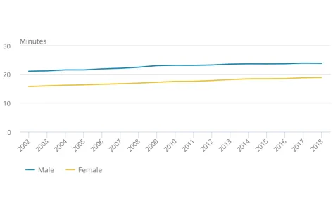
[image:5.595.46.520.209.495.2]

Figure 1 shows how the median commuting time has changed over time for men and women. Results suggest that men tend to commute longer than women. In 2018, the median estimated commuting time was 24 minutes for men and 19 minutes for women. We also find that commuting time has been increasing over time for both men and women. Between 2002 and 2018, the median commuting time has increased by about three minutes for men and women .1

Figure 1: Men tend to commute longer than women

Median commuting time by gender over time, UK, 2002 to 2018

Source: Office for National Statistics – ASHE, 2002 to 2018, own calculations

Notes:

Commuting time is estimated based on the home and work postcode via a trip planner app. It measures the time it takes to go from home to work.

The median is calculated using survey weights.

The shaded areas correspond to the 95% confidence intervals of the weighted median, estimated via bootstrapping.

(6)

1.

2.

[image:6.595.46.522.153.422.2]

3.

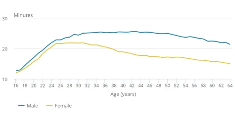
Figure 2: Commuting gap opens up as people reach their mid 20s

Gender disparity in commuting time by age, UK, 2010 to 2018

Notes:

Median is calculated using calibrated weights.

Download data with confidence intervals

(7)

1.

2.

[image:7.595.51.522.179.398.2]

3.

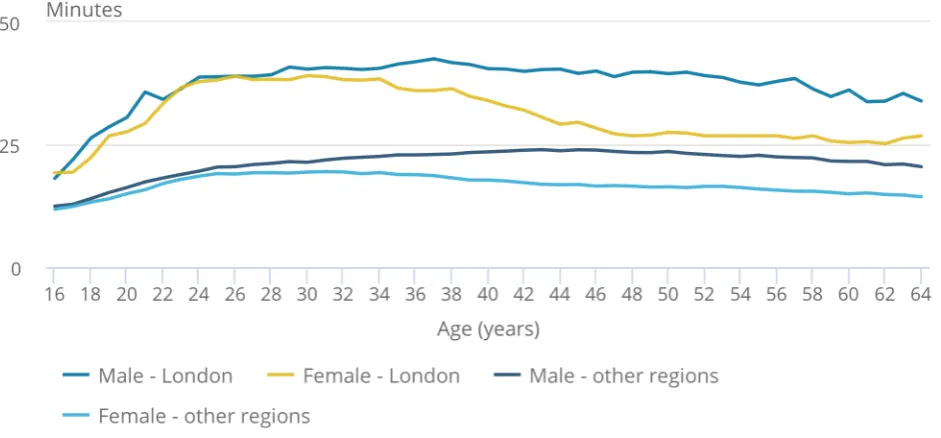
Figure 3: Gender differences are the same in London and across the UK

Gender disparity in commuting time by age, London versus rest of the country, UK, 2010 to 2018

Notes:

(8)

1.

2.

3.

1.

Figure 4: Gross weekly pay begins to diverge when men and women reach their mid 20s

Gender disparity in gross weekly pay by age, UK, 2010 to 2018

Notes:

The median gross weekly pay is expressed in real value for 2018.

The age pattern of the commuting gap mirrors that of the pay gap. This suggests that women may choose jobs with shorter commute, even if they are paid less. This hypothesis is consistent with findings that women tend to favour jobs with greater flexibility and fewer hours worked, at the expense of pay (Mas and Pallais, 2017; Wiswall and Zafar, 2018).

Notes for: The commuting gap

(9)

4 . Do men and women value different job characteristics

differently?

The motivations for leaving one’s job, otherwise known as job separation, vary between men and women. We focus primarily on the effect of pay and commuting distance. Several studies have highlighted that pay has a 1 greater impact on the probability of job separation for men than women in several countries. However, no study has examined whether commuting time affects job separation differently for men and women.

Methodology

We estimate the probability that an individual will leave their job in a given year using a Cox proportional hazard model . We model job separation as a function of commuting time and hourly pay, as well as individual and job 2 characteristics. All the variables in the model are interacted with gender to allow the effect to vary by gender.

More formally, we estimate the following model:

Where h(t) is the hazard for individual i to leave their job at time t, conditional on having remained with the _i employer until time t. h(t) , the baseline hazard, reflects the impact of employment duration t on job separation. ₀ While it may vary with employment duration t, it is assumed to be constant across individuals. As a result, the individual characteristics included in the model are assumed not to affect the baseline hazard. It implies that the effect of individual characteristics is assumed to be time constant; that is, the effect does not vary with time in employment t.

The independent variables of interest are the commuting time in minutes (Ctime ) and the logarithm of hourly _i,t pay (lnhpay ). Following the existing literature, we use the log of hourly pay because the effect of pay on the _i,t decision to change job is likely to be non-linear: a £2 increase in hourly pay at the bottom of the distribution would be expected to have a greater effect on retention than at the top of the distribution. With the log, we assume that a 10% increase in hourly pay has the same effect on retention regardless of the level of pay. In our baseline specification, we include commuting time as a linear term. We then include both pay and commuting time as flexible and undefined functions using penalised splines (Eilers and Marx, 1996). With this approach, the functional form is derived from the data rather than from ad hoc assumptions .3

(10)

age (second-order polynomial)

hours worked (second-order polynomial)

annual leave entitlement (second-order polynomial)

occupation (at two -digit level)

sector (public or private)

number of employees (quintiles) living in an urban area

year

Travel to Work Area4

All covariates are interacted with gender to allow the effects to vary by gender.

If commuting time and hourly pay affect the job separation probability differently for men and women, then we would expect the tests on and to be statistically significant. If the effect of commuting time is stronger for ₁ ₂ women than for men, then we would expect to be positive. If pay has a lesser impact on women’s decisions to ₁ quit their job than men’s, then we would expect to be positive.₂

Interpreting the magnitude of the coefficients is not straightforward. exp( ) reflects by how much the relative ₁ hazards increase for an additional minute of commuting time for men. exp( ) measures the gender difference in ₁ the impact of an additional minute of commuting time on the relative hazards. To help with the visualisation of the results, we display relative hazards for both men and women as a function of commuting time and pay.

The extent to which the estimated coefficients reflect the causal effect of commuting time and pay on the job separation probability depends on whether unobserved heterogeneity is correlated with the dependent variable _i and commuting time and pay. We control for some factors that may be associated with these independent variables and the decision to leave their job (such as occupation, annual leave entitlement, Travel to Work A reas and number of hours). However, there may be unobserved factors that could drive commuting time, pay and decision to change job. For instance, some job conditions (such as flexible working and pressure) and interest in work could influence both the decision to quit one’s job and commuting time. These unobserved factors would bias the estimates of the coefficients.

The direction of the bias depends on how unobserved heterogeneity affects the decision to leave a job and commuting time. We expect unobserved factors that encourage job retention to be associated with longer commuting time. For instance, good working conditions and interest in one’s job are likely to reduce employees’ willingness to leave their job and may be associated with longer commuting time, as they may accept longer commuting times to get a better job. We control for hourly pay and annual leave entitlement but do not capture other non-monetary amenities. We control for public sector as jobs in the public sector may be more flexible. Similarly, having children is expected to reduce willingness to commute and increase the probability of job separation.

(11)

The estimate of the effect of hourly pay ( ) is also likely to be downward biased . However, as we expect hourly ₂ 5 pay to reduce the probability to change job, then is likely to overestimate the true effect of hourly pay. As hourly ₂ pay is likely to have a smaller effect on the decision to leave one’s job for women than for men, we expect to be ₂ negative. If is upward biased, then we would underestimate the difference in the effect of pay between men and ₂ women. As a result, the estimates of and , the two main parameters of interest, are likely to understate the ₁ ₂ gender difference. If the estimates of and are significantly different from zero, then we can be reasonably ₁ ₂ certain that commuting and pay affect women’s decisions to leave their job differently than men’s.

Results

Here we report results from the Cox proportional hazard models used to estimate the effect of commuting time and hourly pay on the probability of men and women leaving their job in a given year. Figure 5 shows estimates of relative hazards for both men and women as flexible functions of commuting time and pay. These estimates are adjusted for age, hours worked, annual leave entitlement, occupation, sector, number of employees and area characteristics (living in an urban area, year and Travel to Work Area). We discuss the robustness of results in more detail in the Appendix, where we present results from different specifications (see Table A1).

(12)

1.

2.

[image:12.595.51.514.85.444.2]

3.

Figure 5: Women place more emphasis on their commute when deciding whether to leave their job, while men prioritise pay

Impact of commuting time and hourly pay on annual job separation rate, UK

Notes:

Post-estimation calculations based on Cox proportional hazard model, which includes penalised splines for commuting time and hourly pay as well as additional covariates for individual and job characteristics: age order polynomial), hours worked order polynomial), annual leave entitlement (second-order polynomial), occupation (at two-digit level), sector (public or private), number of employees (quintiles) living in an urban area, year, and Travel to Work Area.

Models are estimated separately for men and women.

Standard errors clustered at the individual level.

(13)

We use these results to determine the increase in hourly pay that would be needed to compensate for an

increase in commuting time for both men and women. First, we compute the increase in the probability of leaving one’s job caused by a given increase in commuting time. Then, we compute the increase in pay that would be needed to offset the increase in the probability of leaving one’s job caused by an increase in commuting time. For women paid the minimum wage and with a 10-minute commute to accept a commute of an extra 10 minutes, they would need to get a 14.5% pay rise. Men in similar jobs would only need a 9.7% pay increase.

Why do women favour jobs with a shorter commute at the expense of a potentially better paid job? Existing evidence suggests that women work shorter hours and prefer jobs with flexible work schedules because they provide the majority of childcare (Bertrand et al., 2010). Women still provide the majority of childcare in most developed countries, including the UK. Analysis by the Office for National Statistics of time use data show that in

. More

2015, men spent on average 1.9 hours a week doing childcare, compared with 4.7 hours for women

generally, on average women perform more household work than men: women devote 26 hours a week to household work, compared with only 16 hours for men.

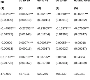
The difference in preference for jobs with short commutes likely also comes from the time pressure imposed by childcare. Unfortunately, the Annual Survey of Hours and Earnings (ASHE) does not have information on whether the individuals have children, therefore we cannot directly test this hypothesis. However, there is some evidence that women’s preference for flexible work schedules results from the burden of childcare (Bertrand et al., 2010). In Table 3, we show estimates of the gender differences in the impact of pay and commuting time on the probability to change job by age group. We do not observe whether the respondents have children, but younger individuals are much less likely to have children. ONS figures shows that the average age of first-time mothers was 28.8

. We find that gender differences in the effect of commuting time are close to zero for those aged

years in 2017

(14)

1.

2.

[image:14.595.235.545.57.333.2]

3.

Table 2: Impact of commuting time and hourly pay on decision to change job, by age

Less than

30 30 to 39 40 to 49 50 to 59 60 and over

(1) (2) (3) (4) (5)

Commuting time 0.00258*** 0.00253*** 0.00251*** 0.00284*** 0.00221***

(minutes) (0.00009) (0.00010) (0.00011) (0.00013) (0.00022)

Log hourly pay -0.44978*** -0.27553*** -0.23605*** -0.15977*** -0.07608***

(0.01222) (0.01146) (0.01204) (0.01393) (0.02247)

Female X commuting time -0.00009 0.00074*** 0.00073*** 0.00058*** -0.00018

(0.00013) (0.00016) (0.00017) (0.00020) (0.00037)

Female X log hourly pay 0.10118*** 0.06319*** 0.03725** 0.01234 0.04384

(0.01722) (0.01662) (0.01760) (0.02041) (0.03569)

Observations 473,900 457,011 502,246 405,330 110,381

Notes

Cox proportional hazard models that control for gender age (second-order polynomial), hours worked (second-order polynomial), annual leave entitlement (second-order polynomial), occupation (at two-digit level), sector (public or private), number of employees (quintiles) living in an urban area, year, and Travel to Work Area. Back to table

All variables are interacted with gender. Back to table

Standard errors clustered at the individual level. Back to table

(15)

1.

2.

3.

4.

5.

6.

Barth and Dale-Olsen (2009) for Norway, Hirsch and Schnabel (2012) for Germany, Webber (2016) for the US.

We only observe the full duration of employment spells for those who have left their job between 2004 and 2018. For those who in 2018 were still employed with the same employer, we cannot observe how they are going to stay in their job. To overcome this “censoring” problem, we use Cox proportional hazard models as is commonly done in the literature (Hirsch and Schnabel, 2012).

In this approach, we estimate separate models for men and women rather than a fully interacted model, because the shape of splines may differ between men and women. We use the psplines package in R.

We show results from specifications with different sets of covariates. Our preferred specification is the one with the highest concordance index.

This may not be the case. While higher hourly pay is likely to be associated with better job conditions, it could also be a compensation for a stressful job. If so, then the coefficient would be biased upward, resulting in underestimating the true effect of pay.

Figure 5 shows the difference in annual probability of job separation for 20-, 30-, 40- and 60-minute-long commutes. For a more comprehensive set of results, see Figure 7 in the Appendix.

5 . Conclusion

Men tend to have longer commutes than women and the commuting gap follows the same age-pattern as the gender pay gap. Commuting time has a greater impact on the decision to leave one’s job for women while hourly rate has a greater impact on men, suggesting that women favour jobs with shorter commutes, at the expense of pay. This is consistent with evidence from the US showing that women tend to favour lower-paying jobs with greater flexibility and fewer hours worked (Mas and Pallais, 2017; Wiswall and Zafar, 2018).

If part of the gender pay gap is caused by women’s willingness to accept lower wages in exchange of greater flexibility and shorter commutes, then closing the gender pay gap would involve addressing the reasons why women favour more flexible jobs. One such reason may be to combine work and family lives, as women provide the majority of childcare as well as care for elderly parents and relatives.

Providing affordable childcare, encouraging flexible working practices and promoting more equal gender norms around care could be the best way to eliminate the gender pay gap.

6 . References

Barth, E., & Dale-Olsen, H. (2009). Monopsonistic discrimination, worker turnover, and the gender wage gap. Labour Economics, 16(5), 589–597. https://doi.org/10.1016/j.labeco.2009.02.004

Bertrand, M., Goldin, C., & Katz, L. F. (2010). Dynamics of the gender gap for young professionals in the financial and corporate sectors. American Economic Journal: Applied Economics, 2(3), 228–255. https://doi.org/10.1257 /app.2.3.228

(16)

Blau, F. D., and Lawrence M. Kahn. 2017. The Gender Wage Gap: Extent, Trends, and Explanations. Journal of Economic Literature, 55 (3): 789–865.

Costa-Dias, M, Joyce, R. and Parodi, F. (2018) The gender pay gap in the UK: children and experience in work, IFS Working Paper 18/02.

Eilers, P. H. & Marx, B. D. (1996). Flexible smoothing with B-splines and penalties. Statistical Science, 11, 89– 121.

Goldin, C. (2014). A Grand Gender Convergence: Its Last Chapter. American Economic Review, 104(4): 1091– 1119. Grambsch P. & Therneau T. (1994), Proportional hazards tests and diagnostics based on weighted residuals. Biometrika, 81, 515–26.

Hirsch, B. (2016). Gender wage discrimination. IZA World of Labor, ISSN 2054-(310), 1–10. https://doi.org/10. 15185/izawol.310

Hirsch, B., & Schnabel, C. (2012). Women Move Differently: Job Separations and Gender. Journal of Labor Research, 33(4), 417–442. https://doi.org/10.1007/s12122-012-9141-1

Kleven, H. J., Landais, C. and Søgaard, J. E. (2019). Children and gender inequality: Evidence from Denmark. American Economic Journal: Applied Economics, forthcoming.

Lagakos SW, Schoenfeld DA (1984) Properties of proportional-hazards score tests under misspecified regression models. Biometrics. 1984 Dec; 40(4): 1037–48.

Lin, D. and Wei, L (1989) The Robust Inference for the Cox Proportional Hazards Model. Journal of the American Statistical Association. Volume 84, 1989 - Issue 408.

Mas, A., & Pallais, A. (2017). Valuing Alternative Work Arrangements. American Economic Review. 107(12), 3722–3759. https://doi.org/10.1257/aer.20161500

Roberts, J., Hodgson, R., & Dolan, P. (2011). “It’s driving her mad”: Gender differences in the effects of commuting on psychological health. Journal of Health Economics, 30(5), 1064–1076. https://doi.org/10.1016/j. jhealeco.2011.07.006

Sulis, G. (2011) What can monopsony explain of the gender wage differential in Italy? International Journal of Manpower, vol. 32(4), pages 446–470, July.

Webber, D. A. (2016). Firm-Level Monopsony and the Gender Pay Gap. Industrial Relations, 55(2), 323–345.

https://doi.org/10.1111/irel.12142

Wiswall, M., & Zafar, B. (2018). Preference for the workplace, investment in human capital, and gender. Quarterly Journal of Economics, 133(1), 457–507. https://doi.org/10.1093/qje/qjx035

(17)

1.

2.

3.

Estimating commuting time in the Annual Survey of Hours and Earnings

(ASHE)

The Annual Survey of Hours and Earnings (ASHE) does not provide direct information on commuting time or mode. However, it contains information on the postcode of the home and workplace of the employee. We use these postcodes to estimate commuting time using a trip planner app, following these steps:

Retrieve the latitude and longitudes of the postcode centroids using the ONS Postcode Directory (ONSPD).

Find the nearest road to the postcodes centroids using Open Street Map (Open Source Routing Machine).

Use the PropeR tool to estimate travel time. We estimated travel time by car or public transport, setting the arrival time at 9am on Monday. Due to technical limitations, this was only possible if the home and work postcodes were in the same or in an adjacent region.

We applied this method to compute travel time by car and public transport for the 1,065,549 combinations of postcodes that we have in the 2002 to 2018 ASHE. Driving time could not be obtained for 137,329 postcodes combinations (12.9%). Travel time by public transport could not be calculated for 340,403 postcodes

combinations (31.9%).

Based on these calculated travel times by car and public transport, we estimated travel time as follows:

Set to “missing driving time” if road distance is lower than the straight-line distance : 10,016 records (0.9%).1 Use driving time if driving time is shorter than public transport, unless the employee lives in inner London, or works in Central London, in which case we use travel time by public transport.

Set to missing if travel time is over four hours – this includes 3,014 records (0.02%).

For postcodes combinations with missing travel time, impute travel time based on a regression model using straight-line distance interacted with region and urban status as predictors.

Cap commuting time to four hours.

(18)

[image:18.595.51.525.196.399.2]

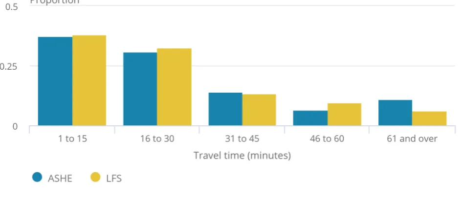
Figure 6: Distribution of commuting times in Labour Force Survey (LFS) and Annual Survey of Hours and Earnings (ASHE) are similar

Commuting time in Labour Force Survey (LFS) and Annual Survey of Hours and Earnings (ASHE), UK

Source: Office for National Statistics – 2017 Labour Force Survey; 2017 ASHE

Sensitivity analysis

(19)

1.

2.

[image:19.595.45.550.44.526.2]

3.

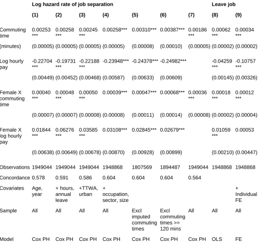
Table A1: Impact of commuting time and hourly pay on decision to change job, different specifications

Log hazard rate of job separation Leave job

(1) (2) (3) (4) (5) (6) (7) (8) (9)

Commuting time 0.00253 *** 0.00258 *** 0.00245 ***

0.00258*** 0.00310*** 0.00387*** 0.00186 ***

0.00062 ***

0.00034 ***

(minutes) (0.00005) (0.00005) (0.00005) (0.00005) (0.00008) (0.00010) (0.00005) (0.00002) (0.00002)

Log hourly pay -0.22704 *** -0.19731 *** -0.22188 ***

-0.23948*** -0.24378*** -0.24982*** -0.04259 ***

-0.10757 ***

(0.00449) (0.00452) (0.00468) (0.00587) (0.00633) (0.00609) (0.00145) (0.00326)

Female X commuting time 0.00040 *** 0.00048 *** 0.00050 ***

0.00039*** 0.00047*** 0.00068*** 0.00036 ***

0.00018 ***

0.00012 ***

(0.00007) (0.00007) (0.00008) (0.00008) (0.00011) (0.00014) (0.00008) (0.00002) (0.00004)

Female X log hourly pay 0.01844 *** 0.06276 *** 0.03585 ***

0.03108*** 0.02845*** 0.02679*** 0.01059 ***

0.00053

(0.00638) (0.00649) (0.00678) (0.00870) (0.00928) (0.00899) (0.00210) (0.00447)

Observations 1949044 1949044 1949044 1948868 1807569 1894487 1949044 1948868 1948868

Concordance 0.578 0.591 0.586 0.604 0.604 0.604 0.564

Covariates Age, year + hours, annual leave +TTWA, urban + occupation, sector, size + Individual FE

Sample All All All All Excl

imputed commuting times Excl commuting times >= 120 mins

All All All

Model Cox PH Cox PH Cox PH Cox PH Cox PH Cox PH Cox PH OLS FE

Notes

All covariates are interacted with a dummy equal to one for women. Back to table

Cox proportional hazard models. Back to table

(20)

1.

2.

[image:20.595.50.519.88.448.2]

3.

Figure 7: Women place more emphasis on their commute when deciding whether to leave their job, while men prioritise pay

Impact of commuting time and hourly pay on annual job separation rate, full results, UK

Notes:

Post-estimation calculations based on Cox proportional hazard models that include penalised splines for commuting time and hourly pay as well as additional covariates individual and job characteristics: age order polynomial), hours worked order polynomial), annual leave entitlement (second-order polynomial), occupation (at two-digit level), sector (public or private), number of employees (quintiles) living in an urban area, year, and Travel to Work Area.

Models are estimated separately for men and women.

Standard errors clustered at the individual level.

(21)

In columns (5) and (6), we show that excluding records with imputed commuting time or commuting times longer than two hours has little effect on the estimates. In column (7), we show that, as expected, omitting hourly pay reduces the estimates of the impact of commuting time on the probability of changing job. This is because pay is positively correlated with job retention and commuting time. In columns (8) and (9), we model the probability of changing as using a linear model and we control for time using log of job tenure. Unlike the Cox model, these models do not account for the fact that the data are censored. In addition, they assume that the impact of job tenure on the job separation probability follows a log-linear relationship. However, the model in column (9) model includes individual fixed effects , which captures time-invariant heterogeneity as this model only exploits the 2 variation within individuals. We show that the results are not substantially different from using a Cox model without individual fixed effects.

We test the proportional assumption for the models presented in column (4) of Table 2 using the test proposed by Grambsch and Therneau (1994), which estimates whether the scaled Schoenfeld residuals and the log of the time variable (tenure in our case) are correlated. We report the results from the tests for our main variables of interest in Figure 8. As is usual with large datasets, we find that the assumption is rejected for commuting time and pay and for the interaction term with gender. This suggests that the impact of pay and commuting time on job separation varies depending on how long the individual has been working for their employer. The violation of the proportional hazard assumption seems more severe for pay than for commuting time. Our models estimate the average effect of commuting time and pay (shown by the solid black line on the graphs). We use robust standard errors (clustered at the individual levels) so the inference is robust to violation of the proportional hazard

(22)

1.

2.

3.

1.

[image:22.595.49.522.43.410.2]

2.

Figure 8: Test of the proportional hazards assumption

Notes:

The blue line is a smoothing of the scaled Schoenfeld residuals.

The black line is the coefficient estimated by the cox model.

If the proportional hazard assumption is met, then the two lines should overlap.

Notes for: Appendix

The straight-line distance is computed based on the postcode centroid, whereas the driving distance is computed based on the nearest road to the postcodes. Therefore, it is possible for the road distance to be lower than the straight-line distance. We therefore only discard travel time if the difference between road distance and the straight-line is lower than minus one kilometre.

A Cox proportional hazard model with individual specific hazard rate could not be run because of the size of our data. Therefore, we used a linear model with individual fixed effects and included the log of job tenure as a control variable.