Evolutionary spectral co-clustering

(1)

Rochester Institute of Technology

RIT Scholar Works

Theses Thesis/Dissertation Collections

2010

Evolutionary spectral co-clustering

Nathan S. Green

Follow this and additional works at:http://scholarworks.rit.edu/theses

This Thesis is brought to you for free and open access by the Thesis/Dissertation Collections at RIT Scholar Works. It has been accepted for inclusion in Theses by an authorized administrator of RIT Scholar Works. For more information, please [email protected].

Recommended Citation

(2)

Evolutionary Spectral Co-Clustering

by

Nathan S. Green

A Thesis Submitted in Partial Fulfillment of the Requirements for the Degree of Master of Science in Computer Science

Supervised by

Dr. Manjeet Rege

Department of Computer Science

B. Thomas Golisano College of Computing and Information Sciences Rochester Institute of Technology

Rochester, New York July 2010

Approved By:

Dr. Manjeet Rege

Thesis Adviser, Department of Computer Science Primary Adviser

Dr. Xumin Liu

Committee Member, Department of Computer Science Reader

Sean Strout

(3)

c

(4)

Abstract

The field of mining evolving data is relatively new and evolutionary clustering is among the

latest in this trend. Presently, there are algorithms for evolutionary k-means, agglomerative

hierarchical, and spectral clustering. These have been excellent in showing the advantages

of using evolving data snapshots for better clustering results. From these algorithms the

key portion of the conversion from static data handling to evolving data handling has been

the addition of the historical cost function. The cost function is what determines whether

or not instances should be moved from one cluster to the next between time-steps based

on the historical cuts made between the instances in the dataset. These cost functions

are then the method by which evolutionary clustering provides smooth transitions as there

is a tunable tolerance for shifts in cluster membership. This also means that transitions

between clusters become much more significant. For example, if an author-word matrix

were clustered over ten years and an author changed clusters part way through the

time-line it is a likely indicator that the author has changed research topics.

Methods for mining evolving data have not yet expanded into co-clustering; for this

reason I have contributed a new algorithm for co-clustering evolving data. The algorithm

uses spectral co-clustering to cluster each time-step of instances and features. Using the

previous example, cluster changes in features (or words) for an author-word matrix is

sig-nificant in that it may indicate a change in meaning for the word. This contribution to the

(5)

List of Figures

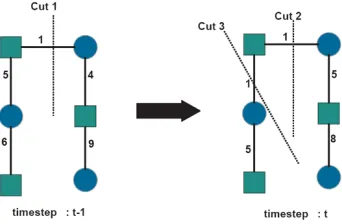
1.1 ESCC uses information from the previous time-step (t − 1) to maintain

cluster membership into the present time (t) in order to provide a smoother transition. Here it can be seen that in order to maintain that membership, despite the evenly weighted cut in the present time, the past comes into effect to makecut 2the better choice at time-stept. . . 2

4.1 t0 is the original data in unclustered and clustered form. t1 shows consis-tency of clustering despite 50 instances of noise per cluster. t2 shows 10 instances added toC2.t3shows 10 instances removed fromC4(highlighted int2). t4 shows cluster stability through a time-step of no change.t5shows 2 features added toC4. t6 shows 1 feature removed from C1 (highlighted int5). t7shows again the stability through an unchanged time-step. . . 15 4.2 t0 is the original data from Figure 4.1. t1 -t3 show the downward shift of

theC4 features andt4 -t7 show the up shift inC5 features. Ultimately the 20 instances were shown to shift fromC4 toC5as expected. . . 17 4.3 t0 is the original data from Figure 4.1. t1 -t3 show the downward shift of

theC4 instances at 2 distinct features and t4 - t7 show the up shift inC5 instances at those features. Ultimately the 2 features were shown to shift fromC4 toC5 as expected. . . 18

4.4 measures for the ESCC clustering on PubMed data. The higher the

F-measure the higher the accuracy of the clustering. This shows that RTH is generally better at sorting out the different clusters. . . 19

4.5 Using the cost formulas from Section 3.1 the two algorithms are measured

(7)

List of Tables

3.1 Symbol Definitions . . . 8

4.1 An outline of the pubmed dataset. . . 19

4.2 ESCC clustering of PubMed. Year 2000. . . 20

(8)

1. Introduction

Clustering refers to the grouping of instances in a dataset based on some similarity criteria

when compared to other instances in the dataset. This is a key method for initial knowledge

mining as no further information is needed than the dataset itself to form clusters. This

pro-vides a way of relating instances in a dataset. Unfortunately, most of the focus in clustering

has been on clustering instances. Rather than focusing on the homogeneous data points

alone we can further our knowledge by including the features in our clustering through

co-clustering, creating a heterogeneous set of clusters. This research area has been trending

upward as there are many applications for relating heterogeneous types [10, 19, 7, 16].

Co-clustering of a dataset is a method by which instances and features can be

simul-taneously clustered in order to better relate the instances and features. In order to run a

co-clustering algorithm on a dataset the data needs to be well formed for the operation. In

this case “well formed” refers to a data set with data akin to an incidence matrix (having

more than one connection) or a co-occurrence matrixM where rows and columns represent

the types to be interrelated through co-clustering. In this case an entry in the matrix Mij

would have a value representing the relationship between the instance type at row i and

the feature type at column j. From this weight matrix I was able to manipulate the data to

shrink it into more manageable form, keeping instance and feature ties relative to the

orig-inal dataset. These manipulations are part of the co-clustering algorithm [14]. This also

allows the clustering algorithm to avoid the dimensionality curse [1, 11] as all dimensions

are considered. The co-clustering problem has also been modeled as a bipartite graph by

[7] and [17]. Optimizations for data handling of large datasets were found using matrix

factorization and block value decomposition as proposed in [4] and [13], respectively.

Fur-thermore, the problems addressed using co-clustering are wide spanning. In biology, gene

(9)

Dhillon [7] proposed a bipartite clustering algorithm tested with documents and words.

Lastly, in [16] image understanding problems were addressed using co-clustering allowing

researchers to further analyze image content. However, all of these efforts have been on

static data. None of these take into account the passage of time and knowledge that can be

[image:9.612.224.395.202.314.2]

gained by observing data as it evolves.

Figure 1.1: ESCC uses information from the previous time-step (t−1) to maintain cluster membership into the present time (t) in order to provide a smoother transition. Here it can be seen that in order to maintain that membership, despite the evenly weighted cut in the present time, the past comes into effect to makecut 2the better choice at time-stept.

To the best of my knowledge there are no efforts toward the creation of evolutionary

data mining algorithms for the purpose of co-clustering. In this thesis I present

evolution-ary spectral co-clustering (ESCC) for co-clustering of evolving data. An example of two

evolutionary time-steps is shown in Figure 1.1. This figure shows a decision swayed by

the incorporation of historical data. In order to incorporate historical data it is necessary to

develop an historical cost function. The cost function in this case is created to handle the

evolving instances and features for co-clustering. The resulting matrices formed from these

cost functions are decomposed using spectral value decomposition (SVD) and the k-means

clustering algorithm is then applied to obtain the desired number of clusters [14].

In order to show the features of this algorithm I perform extensive experiments on three

different synthetic datasets and a real world dataset from the PubMed database. The first

demonstrates the algorithm’s ability to handle noise, added and removed instances, added

and removed features, and the consistency across similar time-steps. The second synthetic

(10)

Finally, the third synthetic data set shows the algorithm’s ability to track features through

cluster shifts over time. Additionally, in order to show the accuracy of the algorithm a

real world data set is used. The dataset consists of authors and words from two separate

subjects in the PubMed database over the last ten years. This dataset is clustered and cluster

assignments are compared to the original subjects.

Thus the contributions of this thesis are outlined as follows:

• Anew algorithm (ESCC)to the field of evolutionary data mining.

• Two new historical cost functionsdesigned for co-clustering of heterogeneous data.

• The method forcreating and formattingheterogeneous data.

• Experimentally provingthe accuracy of ESCC.

The rest of the thesis is organized as follows. Chapter 2 provides a literature review of

papers relevant to the thesis. Chapter 3 will show the details of the algorithm for this thesis.

Chapter 4 details the experiments used in this thesis. Chapter 5 provides conclusions drawn

from the experiments and details potential future work in this new field. Finally, Chapter 6

(11)

2. Background and Related Work

While the concept of mining evolving data is relatively new, the concepts on which it is built

are very well researched. As outlined below, many of the concepts previously researched

and experimented upon will provide the building blocks for the algorithm and experiments

that follow within this thesis.

2.1 Evolutionary Clustering

The concept of evolutionary clustering came into being in 2006 with the publication by

Chakrabarti et al. [3]. This is not to be confused with any genetic algorithm[8] as the data

itself is evolving and the algorithm is simply clustering it. An additional disambiguation is

necessary in that many previous datasets have taken time into account with clustering, but

not as a smoothing feature. The difference lies in the objective: where previous clustering

efforts looked for information about the temporal data, Chakrabarti et al. looked for

infor-mation about data which was clustered over multiple time-steps. Further disambiguations

are necessary in regard to incremental clustering [18, 6] and constraint based clustering

[6, 2], also known as semi-supervised learning. Incremental clustering focuses on the up-dating of centroids [9] or other data structures through each iteration of the algorithm.

Through each update the focus is on the new clustering instead of the cluster membership

of previous data points. Constraint-based clustering requires further information beyond

simply having the data. In addition to the data some domain knowledge is needed to

inte-grate heuristic decisions within the algorithm. These heuristics can be presented as hard constraints[20] wherein instances must or cannot be linked orsoft constraints[12] wherein knowledge is used as an initial grouping.

(12)

handle evolving data. The addition to the field which will be used in this research includes

the cost functions to properly cluster at each time-step with respect to previous steps. These

were the history cost–how similar clustering attis tot−1–and the snapshot quality–how well the clusters match the desired clusters. These are extended in [5] wherein further work

is done to smooth the time shifts.

The authors of [5] extend the work in [3] to use the spectral clustering algorithm. Along

with this addition to evolutionary clustering, further work was done to produce historical

cost and snapshot cost functions. These are what drive decisions like the one shown in

Figure 1.1 and what will be implemented for co-clustering in this thesis.

In a recent unpublished work, Wang et al., use low level matrix factorization to achieve

a more efficient evolutionary clustering algorithm on large scale data. As stated in [11] all

clustering efforts suffer from potential dimensionality curse as the number of dimensions

exceed 16. The framework introduced in [21], Evolutionary Clustering based on

low-rank Kernel matrix Factorization (ECKF), is one which is claimed to be extensible to any

evolutionary clustering problem. This work also adds the intelligence to decide whether

or not a new clustering is necessary based on the underlying changes to the data at each

time-step.

2.2 Spectral Co-Clustering

Spectral clustering is intended to be a very simple algorithm for clustering many different

sized data sets with accuracy greater than that of the k-means algorithm and often greater

than many other traditional clustering algorithms. Its implementation relies heavily on

matrix computation, graph Laplacians, and the k-means algorithm [14].

There are multiple spectral clustering algorithms making use of unnormalized and

nor-malized Laplacians, graph cutting, random walks and perturbation all outlined in [14]. The

tutorial paper provides an excellent overview of the algorithm, it’s uses and how to

(13)

understanding of the spectral clustering algorithm and where to modify it to handle

evolv-ing data.

The development of co-clustering requires an understanding that the left and right

singular vector matrices will present differently when the weight matrix is normalized.

This normalization will properly incorporate the features. The following method from [7]

was used to normalize the weight matrix starting with the generalized eigenvalue problem

Lz =λDz.

L=





D1 −A

−AT _D

2   (2.1) D =  

D1 0

0 D2



 (2.2)

from [7] equations 2.1 and 2.2 can be rewritten to obtain the normalization formula

Wn =D

−1 2

1 W D

−1 2

2 (2.3)

which creates the weight matrix used for co-clustering in ESCC.

The ability to cluster on multiple data sets at once is a most desirable faculty for a

clustering algorithm. This provides the ability to gain further insight concerning the

rela-tionship between separate data sets. The common one-way clustering effort works well,

but restricts what information can be gleaned from multiple data sets. The one-way

clus-tering effort also suffers from the dimensionality curse [1], wherein high dimensioned data

is much more difficult to cluster.

Co-clustering serves the purpose of clustering the individual data sets through relating

them to each other. This partially undoes the dimensionality curse in that further refinement

of clusters is made through relating the data points to the attributes and back again [11]. For

instance with text mining of document sets and word sets the two data sets can be clustered

(14)

shown further in [7].

Dhillon starts his research with the graph partitioning problem for the purpose of

clus-tering dyadic data sets. As of 2007 it was a novel concept to treat the data sets as vertices

in a graph. The edges connecting these different data sets would represent a relationship

between the two and the weight of the edge would represent the strength. With clustering

this graph the goal is to partition along the least weighted edges in order to best separate

the clusters.

Dhillon uses documents and words as the separate data sets the same way that was used

in [13]. The graph partitioning method for co-clustering works to relate words to documents

thus also clustering words to each other and the same for documents. As with previous

papers, this is the goal of co-clustering. The spectral partitioning method, however, is more

scalable than the previous work. Experiments from the paper show that the spectral graph

partitioning method can discern a small amount of documents from other clusters of larger

sets of documents.

From this research it has shown that there is a lack of co-clustering on evolving data.

The research by Chi et al. on spectral clustering of evolving data combined with the

re-search by Dhillon on using spectral clustering on bipartite graphs gives an excellent

(15)

3. ESCC

This is a novel algorithm to the field and will be described here in detail. First, the

algo-rithm not only handles the insertion and deletion of instances, but features as well. This is

necessary for changes over time concerning co-clustering. Next, the algorithm shows

re-sistance to changes between time-steps in the instances as shown before [5], and shows this

for changes in features as well. Finally, the algorithm shows movements of data between

time-steps in the instances as well as the features.

Symbol Definition

At A matrix for time-stept

AT_,_ZT_,_{. . .} _{The transpose of the given matrix} A0,W0,. . . A manipulation of the given matrix

Wmxn A data matrix of weights of sizemxn W(i,j The value of the weight for instanceigiven featurej W(i,:),W(:,i) The row or column atifrom matrixW, respectively

W_wrt0 ₍_W₎ The matrixW0 with respect toW (Definition 1)

D A diagonal matrix described in Section 2.2

D1,D2 Diagonal matrices for instances and features respectively

Dn,t Diagonal matrix for the given dimensionnand time-stept

k Number of clusters

Cn Cluster numbern

t Time-step

µ Mean value

~

d A vector of indices having differences resulting from the comparison of two matrices

d An index ind~

svd The singular value decomposition function

n..p,2..4 For all valuesntop,[2,3,4]

α,β Constants for tuning the algorithm RTC|RTH Choose RTC algorithm or RTH algorithm

Xu,Xv Right and left singular vectors respectively ordered by descending eigenvalue

[image:15.612.93.511.326.619.2]

Zu,Zv Computed cuts for instances and features respectively

(16)

3.1 RTC vs. RTH

I present two methods for including past time-step clustering into the present. These

meth-ods are each referred to as the evolutionary method by which clusters are chosen from

time-step to time-step. The first of these methods is Respect To the Current (RTC), wherein

the present clustering quality (CQ) is of most importance and historical cost (HC) is

cal-culated with only one previous time-step. The second, is Respect To Historical (RTH).

RTH attempts to keep instances and features tied to the same clusters between time-steps,

therefore this method uses all previous time-steps when calculating historical cost. In this

case the best example can be given through Figure 1.1 where either evolutionary method

would choose cut 2, however if the weight of the edge on cut 2 were higher the two would

disagree. If making cuts with RTC the optimal clustering for the present time will be

cho-sen (cut 3) within a margin of tolerance dictated by the values chocho-sen for the constants,α

andβ, shown in Equation 3.1. On the other hand when making cuts with RTH within the

tolerance cut 2 would still be chosen as it reduces the error in historical clustering.

ECt =k−trace

Xv_tT (αCQt+βHCt)Xut

(3.1)

The accuracy of the clustering for each of these is determined by the cost of each

time-step, this is known as theevolutionary cost. The evolutionary cost (EC) is computed through a summation of the clustering quality and the historical cost. Historical cost being

the added negative weight for choosing a cut that causes a cluster change. RTC and RTH

have differing cost functions as each are modeled for different purposes. The CQ and HC

for RTC is defined as in Equation 3.2 and the CQ and HC for RTH is defined in equation

3.4. AsXu andXv are created from the left and right singular vectors from all previous

time-steps, the HC for RTH is more tightly connected to the past clustering choices. In

(17)

CQt=αD

−1₂

1,t WtD

−1₂

2,t

HCt=βD

−1 2

1,t−1Wt−1D

−1 2

2,t−1 (3.2)

(3.3)

CQt=αD

−1 2 1,t WtD

−1 2 2,t

HCt=βXut−1XvTt−1 (3.4)

(3.5)

The aim is to minimize these costs to give the best possible cut through the data. The

minimization is achieved by using the topk singular vectors from the left (Xut) and from

the right (Xvt) of the singular value decomposition performed in Algorithm 2. CQtrefers

to the cluster quality at time t, while HCt refers to the historical cost at time t. These

measures differ in thatCQmeasures the quality of the present clustering as if it were static

data andCH measures the cost of change from the previous time-step to the present.

3.2 Handling Data Changes

The balanced insertion discussed previously is meant to make the dimensions of each

time-step comparable while not compromising the cluster assignments of other instances. This

need to handle changes in the data dimensions over time requires a new construct to be

created. This new construct is the WRT construct.

(18)

of Algorithm 1.

In order to accomplish this when adding instances or features to the past different

meth-ods are used based on the selection of RTC or RTH. In the case of RTC, where present

quality is most important, the inserted row or column receives the average of the whole

matrix at present time for each cell. In the case of RTH the inserted row or column receives

the average of the new row or column in each cell.

The easier of the two operations is removal of instances or features from past

time-steps. This occurs when an instance or column in the past matrices is no longer present in

the current time-step. In this case the instance or column can be removed from the past in

(19)

Algorithm 1Generate WRT Matrices Algorithm

1: INPUT: W_1:0_t(history), Wt(present), RTC|RTH { // history contains all weight matrices previous to present,presentcontains the current time-step for which this With Respect To (WRT) Matrix is being created, RTC—RTH is the evolutionary method chosen}

2: OUTPUT:Wwrt:t

3: METHOD:{// Start with removal of differing rows and columns} 4: fort0 ←1..length of historydo

5: d~←W_t00 ∈/ W

6: W_t0

wrt(Wt)

←W_t00 −W_t,₍_d,~_:)

7: d~←W0T

t ∈/WT

8: W_t0

wrt(Wt)

←W_t00T−WT t,(:, ~d)

T

9: end for

{// Make additions next, these will be based on the evolutionary method} {// Start with Row/Instance addition}

10: fort0 ←1..length of historydo

11: d~←W /∈W0 t0

12: ifRTCthen

13: for alldifferencesd~do

14: insert←µW_t00

15: AddinserttoW_t0

wrt(Wt),(d,:)based on its ID 16: end for

17: else ifRTHthen

19: insert←µW_t0_,₍_r_~

d)

20: AddinserttoW_t0

wrt(Wt),(d,:)

based on its ID 21: end for

22: end if

23: end for

{// Column/Feature addition next} 24: fort0 ←1..length of historydo

25: d~←W /∈W_t00

26: ifRTCthen

28: insert←µW0 t0

29: AddinserttoW_t0

wrt(Wt)

31: else ifRTHthen

33: insert←µW_t0_,₍_c_~

d)

34: AddinserttoW_t0

wrt(Wt),(:,d)

36: end if

(20)

3.3 Piecing the algorithm together

As stated previously, Xu and Xv are left and right singular vectors consisting of

infor-mation from all previous time-steps. These take different forms based on the evolutionary

method chosen. If working with RTC the calculations forXuandXv are shown in

Equa-tion 3.6 and similarly for RTH they are shown in EquaEqua-tion 3.7. The difference lies in the

statements tied to the coefficient β. Being connected with only the last time-step is the

role of RTC and shown in the calculation for EC as well. However, a connection with all

previous time-steps is shown with RTH through its recursive reference.

[Xut, Xvt] =svd

h

αWt+βD−

1 2 1,t−1W D

−1 2 2,t−1

i

(3.6)

[Xut, Xvt] =svd

αWt+βXut−1XvtT−1

(3.7)

wherein all references to time-steptare of the formtwith respect to the current time-step.

For example, if there is an instance increase between time-stept−1andt,t−1with respect totwould have the additional instances as a balanced insertion to the matrix.

The collected singular vectors must be passed to k-means in order to generate clusters

for each time-step. The final matrixZ is the result of the following

Z =   D− 1 2

1,t Xut(2..dlog2ke)

D−

1 2

2,t Xvt(2..dlog2ke)



 (3.8)

where Xut andXvt are comprised of all left and right singular vectors, respectively, for

time-stept, andk remains the number of clusters.

The result of putting all of this together is represented in the ESCC algorithm shown in

(21)

Algorithm 2ESCC Algorithm

1: INPUT:Wmxnxt,k, and RTC|RTH{//W is anmxnxtmatrix wheretis the number of time-steps,k

is the number of clusters}

2: OUTPUT:Cluster assignments for each time-step 3: METHOD:

4: forall time-stepsdo

5: forall time-steps previous to the currentdo

6: create corresponding past matrices with respect to the present time-step using Algorithm 1 7: end for

8: forall time-steps previous to the currentdo

9: ifRTCthen

10: use equation 3.6 for SVD 11: else ifRTHthen

12: use equation 3.7 for SVD 13: end if

14: combine left and right singular vector matrices using equation 3.8 15: runk-means on resulting matrix

16: end for

17: end for{// The firstmcluster values for each time-step represents the instance clustering and the trailing

(22)

4. Experiments

Two sets of experiments were run to determine the validity and effectiveness of this

al-gorithm. The first set of experiments involved a synthetic dataset designed to show the

different functions of the algorithm. The second shows the accuracy of the algorithm on

real world data using a dataset from the widely used PubMed database of medical research

[image:22.612.92.530.306.399.2]

papers.

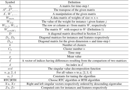
Figure 4.1: t0 is the original data in unclustered and clustered form. t1 shows consistency of clustering despite 50 instances of noise per cluster. t2shows 10 instances added toC2. t3 shows 10 instances removed fromC4 (highlighted int2). t4shows cluster stability through a time-step of no change. t5 shows 2 features added to C4. t6 shows 1 feature removed fromC1 (highlighted int5). t7 shows again the stability through an unchanged time-step.

4.1 Synthetic Data

Three different synthetic datasets were used to show the features of the algorithm. The

first, shown in 4.1.1, demonstrates the algorithm’s ability to handle noise, added instances,

removed instances, added features, and removed features as well as the consistency across

similar time-steps. The second (4.1.2) synthetic data set shows the algorithm’s ability to

track instances through cluster shifts over time. Finally, the third (4.1.3) synthetic data set

(23)

4.1.1 Synthetic Demonstrations

I have constructed a synthetic dataset with 8 time-steps and 5 clusters of 200 instances each

having 10 assigned features. The initial time-step and 5 clusters were formed by creating

5 ascending groups of data sampled from 5 normal distributions. Each normal distribution

was guaranteed to be distanced from the previous through an augmentedµvalue added to

the previousµ. Therefore, if a cluster,Cn, has an assignedµit is represented byµnwhere

n is the cluster number, then the distributions are determined by µn = µn−1 + 5·n +R whereRis a random integer bound by[0−100]. For all distributionsσ= 1.

To form time-stept1 Gaussian noise was added to 50 instances per cluster. It is shown

in Figure 4.1 that t0 and t1 are unchanged, despite the added noise. Next, int2 instances

were added toC2 using a selection of values from a normal distribution having aµ =µ2.

The figure shows that the additional instances were added and appropriately clustered as

indicated by the green shaded box. To show the opposing action int3instances are removed

from C4. From the figure it can be seen that all clusters remain unchanged andC4 has a

smaller block size. This was also indicated int3 as the instances that will be removed are

highlighted in blue. In t4 the data is unchanged, simulating the stability of the clustering

between time-steps.

Until this point the algorithm has behaved as any previous evolutionary algorithm

would, however with t5 features will be added to the dataset inC4 using values selected

from a normal distribution having aµ =µ4. The figure shows that the additional features

have not affected the clusters and the resulting new columns were correctly clustered as

in-dicated by the green box around the column of data in Figure 4.1 time-stept5. Int6features

were removed fromC1and the figure shows again that the clustering is unaffected and the

block for C1 is diminished. This was also indicated in t5 by the blue shading around the

(24)

[image:24.612.224.394.88.263.2]

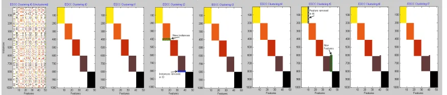
Figure 4.2: t0 is the original data from Figure 4.1. t1 -t3 show the downward shift of the

C4 features andt4 -t7 show the up shift inC5 features. Ultimately the 20 instances were shown to shift fromC4 toC5as expected.

4.1.2 Synthetic Instance Drift

Using the same initial time-step and 5 cluster distribution from section 4.1.1, a group of 20

instances were incrementally modified at each time-step, up to 8, to denote a cluster shift

of the instances. Figure 4.2 shows the time series of clustered data. It can be seen att3 that

the instances are discolored denoting a drop in value and int4the instances change clusters

when values for the next cluster’s features begin rising.

4.1.3 Synthetic Feature Drift

In the same manner as the previous example, a feature shift is shown. Two features were

chosen fromC4 to have their values lowered inC4 and raised inC5. Figure 4.3 shows the

progression over each time-step. As with the last experiment the color change indicates

diminished values and at t3 the values correlated withC5 begin increasing and the cluster

(25)

[image:25.612.224.394.88.262.2]

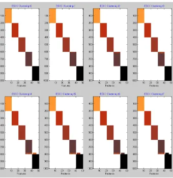
Figure 4.3: t0is the original data from Figure 4.1. t1-t3show the downward shift of theC4 instances at 2 distinct features andt4-t7show the up shift inC5instances at those features. Ultimately the 2 features were shown to shift fromC4toC5 as expected.

4.2 Real Data

To evaluate the accuracy of ESCC on real data, I selected a widely used database of medical

papers: PubMed1_{. The PubMed dataset was constructed from two searches of highly}

re-searched topics in the medical field: schizophrenia treatment and stem cell research. Each

search was limited to English texts published between 1990 and 2009 having authors and

abstracts. The papers were then parsed by year to obtain author-word matrices for each

year containing both subjects. Common stop words were removed and all words were

stemmed using Porter’s suffix-stripping algorithm [15]. Authors and words were assigned

unique IDs tied to the first occurrence based on the year the author or word was used and

the subject matter, respectively. These unique ids are used in the generation of the WRT

matrices as demonstrated in Algorithm 1. Authors that had published less than three papers

in the time-span were removed from the dataset and words occurring less than 30 times

throughout the abstracts were also removed. This resulted in 10 data time-steps consisting

of information from 64,320 papers, 17,731 unique authors, and 8,541 unique words these

are described by year in Table 4.1.

(26)

[image:26.612.219.399.87.226.2]

Year # Papers # Authors # Words 2000 2817 4907 6750 2001 2792 5254 6860 2002 3486 6220 7117 2003 3698 6734 7205 2004 4059 7244 7327 2005 4059 8023 7452 2006 4376 7984 7286 2007 4690 8365 7302 2008 4962 8234 7328 2009 5074 7988 7304

Table 4.1: An outline of the pubmed dataset.

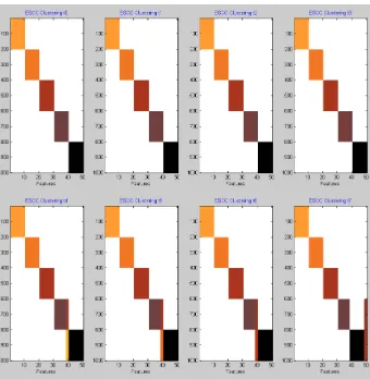
Figure 4.4: F-measures for the ESCC clustering on PubMed data. The higher the F-measure the higher the accuracy of the clustering. This shows that RTH is generally better at sorting out the different clusters.

Each year represented was run using the RTC and RTH framework. Theαandβvalues

were 0.7 and 0.3 respectively. The following series of confusion matrices and top words

from the respective clusters show the ability for ESCC to cluster authors appropriately as

well as the words through each time-step. As can be seen in Figure 4.4 RTH outperforms

RTC in nearly each time-step. This is because authors do not often change subjects, despite

the enormous amount of noise in the words utilized in each abstract. Furthermore, Figure

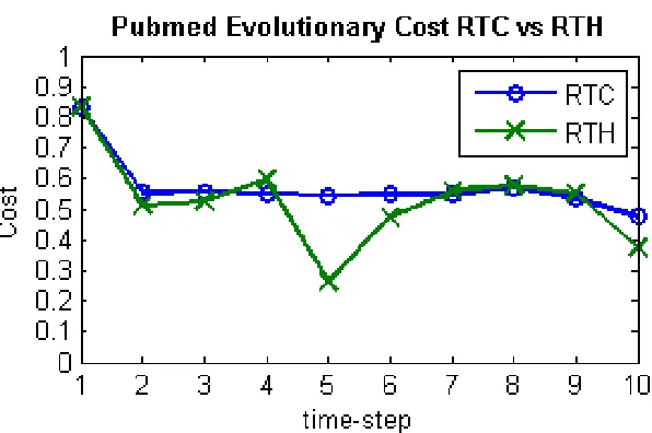
4.5 shows that RTH maintains historical cluster membership as expected and better than

the RTC counterpart.

[image:26.612.166.460.263.428.2]

(27)

RTC SchizR StemCell

Auth1: 1558 432

Auth2: 52 2864

RTH

Auth1: 1558 432

Auth2: 52 2864

W1: disord drug mental psychiatri stress

W2: allogen repopul graftversushost leukem posttranspl

Table 4.2: ESCC clustering of PubMed. Year 2000.

RTC SchizR StemCell

Auth1: 1805 374

Auth2: 609 2465

RTH

Auth1: 1706 473

Auth2: 52 3022

RTC

W1: treatment schizophrenia disord depart human W2: colonyform gvh osteoclast transfus leukem RTH

W1: treatment effect schizophrenia disord psychiatr W2: marrow bone transplant blood hematopoiet

RTC SchizR StemCell

Auth1: 1848 578

Auth2: 79 3714

RTH

Auth1: 1834 592

Auth2: 75 3718

RTC

W1: treatment effect schizophrenia univers depart W2: patient studi transplant bone stem

RTH

W1: treatment schizophrenia symptom clinic antipsychot W2: patient transplant bone stem blood

RTC SchizR StemCell

Auth1: 2199 613

Auth2: 149 3772

RTH

Auth1: 2172 640

Auth2: 67 3854

RTC

W1: treatment schizophrenia result disord ptsd W2: patient studi bone univers depart

RTH

W1: treatment schizophrenia result disord ptsd W2: patient studi bone transplant univers

RTC SchizR StemCell

Auth1: 2492 657

Auth2: 306 3788

RTH

Auth1: 2349 755

Auth2: 118 3976

RTC

W1: patient treatment result effect disord W2: studi bone transplant univers clinic RTH

W1: patient treatment disord symptom antipsychot W2: studi bone transplant univers clinic

(28)

RTC SchizR StemCell

Auth1: 2740 674

Auth2: 620 3988

RTH

Auth1: 2665 749

Auth2: 746 3862

RTC

W1: treatment disord group symptom antipsychot W2: cell patient studi bone result

RTH

W1: patient studi treatment schizophrenia mai W2: cell bone result marrow transplant

RTC SchizR StemCell

Auth1: 2784 718

Auth2: 792 3689

RTH

Auth1: 2635 856

Auth2: 160 4332

RTC

W1: studi schizophrenia result ptsd effect W2: patient treatment bone stem marrow RTH

W1: patient treatment univers symptom clinic W2: cell studi bone result stem

RTC SchizR StemCell

Auth1: 3074 641

Auth2: 1395 3254

RTH

Auth1: 3008 719

Auth2: 1400 3237

RTC

W1: treatment effect disord depart clinic W2: allogen epc gvhd osteoblast hmsc RTH

W1: treatment effect disord clinic symptom W2: studi bone result univers group

RTC SchizR StemCell

Auth1: 2942 810

Auth2: 1273 3208

RTH

Auth1: 2996 756

Auth2: 1325 3156

RTC

W1: treatment result disord ptsd univers W2: epc bmsc engraft gvhd graftversushost RTH

W1: patient treatment result disord ptsd W2: cell studi bone effect univers

RTC SchizR StemCell

Auth1: 3589 2

Auth2: 4381 15

RTH

Auth1: 2587 1004

Auth2: 133 4263

RTC

W1: patient studi treatment schizophrenia ptsd W2: colonyform thalidomid feeder bdlsc gfplabel RTH

W1: patient treatment disord group clinic W2: cell studi result effect msc

(29)

[image:29.612.164.462.91.289.2]

Figure 4.5: Using the cost formulas from Section 3.1 the two algorithms are measured for accuracy and maintaining historical clustering. A lower cost value indicates a better clustering in regard to maintaining history. As can be seen in the graph, I have found that RTH generally performs better than RTC.

within the medical field. The RTH algorithm shows a better clustering through the end

while the RTC algorithm did not finish as well as shown in Table 4.11. As more authors

are introduced to the set, the words are fairly constant because of the constraint that each

be used 35 or more times within the selected abstracts. This meant that the clusters became

more saturated and blended the lines making the distinctions more difficult over time.

How-ever, by the evolutionary cost graph in Figure 4.5 where a maximum cost has a value of 2,

the given costs show low changes in cluster membership, reducing noise. Observing the

selection of top words clustered with each set shows that the co-clustering element of this

(30)

5. Conclusion

I have presented a new algorithm to the field of evolutionary data mining. The research

shows it as novel and contributing a new direction to this field. Evolutionary co-clustering

will give a new option for mining of data collected over time with reduced noise and

aug-mented incorporation of past data. The synthetic experiments show that the algorithm

performs as it should for each of the features claimed and tested. Finally, the algorithm

shows that with enough time and resources clusters will form showing accurate

distinc-tions between separate groups of data.

Further research is necessary to determine the full range of uses for this new algorithm

as this is a new direction for the field of mining evolving data. This research may lead

to more datasets properly suited for the evolutionary mining process. Currently it is very

difficult to find a dataset with a focus on time-steps. An interesting direction would be

datasets with time-steps which are less than a year in length, something like a blog server

or a mashup of RSS feeds with daily updates, users, and words to be clustered. In any case,

more data well-formed for evolutionary data mining would be an excellent next step.

Additionally, there are far more efficient, much more complicated algorithms that could

also be converted to handle evolving data. This research provides a road map for those that

would venture to take on the endeavor of creating a novel algorithm in the evolving data

mining field. Incorporating matrix factorization or block value decomposition were outside

the scope of this research, but would make an excellent comparison for the research within

(31)

6. Acknowledgments

A grand thank you to Professor Rege, my committee, and Patrick Saeva and Peter Erhardt

of the RIT Office of Development for their assistance with this thesis. I was unable to use

the dataset provided by them for this research, however their assistance was most

appre-ciated. Additionally, much thanks to Vickie for making me sit down and work when all I

wanted to do was run CSH. My thanks also goes to the Research Computing group at the

Rochester Institute of Technology for the compute time that could not be accomplished by

(32)

Bibliography

[1] Charu C. Aggarwal. On k-anonymity and the curse of dimensionality. In VLDB

’05: Proceedings of the 31st international conference on Very large data bases, pages 901–909. VLDB Endowment, 2005. ISBN 1-59593-154-6.

[2] Mikhail Bilenko, Sugato Basu, and Raymond J. Mooney. Integrating

con-straints and metric learning in semi-supervised clustering. In ICML ’04:

Proceedings of the twenty-first international conference on Machine learning,

page 11, New York, NY, USA, 2004. ACM. ISBN 1-58113-828-5. doi:

http://doi.acm.org/10.1145/1015330.1015360.

[3] Deepayan Chakrabarti, Ravi Kumar, and Andrew Tomkins. Evolutionary clustering. In KDD ’06: Proceedings of the 12th ACM SIGKDD international conference on Knowledge discovery and data mining, pages 554–560, New York, NY, USA, 2006. ACM. ISBN 1-59593-339-5. doi: http://doi.acm.org/10.1145/1150402.1150467.

[4] Yanhua Chen, Lijun Wang, and Ming Dong. Non-negative matrix factorization for

semi-supervised heterogeneous data co-clustering. IEEE Transactions on Knowledge

and Data Engineering, 99(PrePrints), 2009. ISSN 1041-4347.

[5] Yun Chi, Xiaodan Song, Dengyong Zhou, Koji Hino, and Belle L. Tseng.

Evolution-ary spectral clustering by incorporating temporal smoothness. InKDD ’07:

Proceed-ings of the 13th ACM SIGKDD international conference on Knowledge discovery and data mining, pages 153–162, New York, NY, USA, 2007. ACM. ISBN 978-1-59593-609-7. doi: http://doi.acm.org/10.1145/1281192.1281212.

[6] Ian Davidson, S. S. Ravi, and Martin Ester. Efficient incremental constrained

cluster-ing. InKDD ’07: Proceedings of the 13th ACM SIGKDD international conference on

Knowledge discovery and data mining, pages 240–249, New York, NY, USA, 2007. ACM. ISBN 978-1-59593-609-7. doi: http://doi.acm.org/10.1145/1281192.1281221.

[7] Inderjit S. Dhillon. Co-clustering documents and words using bipartite

(33)

SIGKDD international conference on Knowledge discovery and data mining, pages

269–274, New York, NY, USA, 2001. ACM. ISBN 1-58113-391-X. doi:

http://doi.acm.org/10.1145/502512.502550.

[8] Michael Goebel and Le Gruenwald. A survey of data mining and knowledge

discov-ery software tools.SIGKDD Explor. Newsl., 1(1):20–33, 1999. ISSN 1931-0145. doi:

http://doi.acm.org/10.1145/846170.846172.

[9] Chetan Gupta. Genic: A single pass generalized incremental algorithm for

clustering. SIAM International Conference on Data Mining, 2004. URL

http://citeseerx.ist.psu.edu/viewdoc/summary?doi=?doi=10.1.1.1.5567.

[10] Daniel Hanisch, Alexander Zien, Ralf Zimmer, and Thomas Lengauer. Co-clustering

of biological networks and gene expression data. Bioinformatics, 18(1):145–154,

2002.

[11] Jacob Kogan, Charles Nicholas, and Marc Teboulle. A survey of clustering data

min-ing techniques. Springer Berlin Heidelberg, 2006.

[12] M. H. C. Law, A. Topchy, and A. K. Jain. Clustering with soft and group constraints.

LECTURE NOTES IN COMPUTER SCIENCE, 2004.

[13] Bo Long, Zhongfei (Mark) Zhang, and Philip S. Yu. Co-clustering by

block value decomposition. In KDD ’05: Proceedings of the eleventh ACM

SIGKDD international conference on Knowledge discovery in data mining, pages

635–640, New York, NY, USA, 2005. ACM. ISBN 1-59593-135-X. doi:

http://doi.acm.org/10.1145/1081870.1081949.

[14] Ulrike Luxburg. A tutorial on spectral clustering. Statistics and Computing, 17(4): 395–416, 2007. ISSN 0960-3174. doi: http://dx.doi.org/10.1007/s11222-007-9033-z.

[15] M. F. Porter. An algorithm for suffix stripping. Morgan Kaufmann Publishers Inc.,

San Francisco, CA, USA, 1997. ISBN 1-55860-454-5.

[16] Guoping Qiu. Image and feature co-clustering. Pattern Recognition, International

Conference on, 4:991–994, 2004. ISSN 1051-4651.

(34)

words using bipartite isoperimetric graph partitioning. In ICDM ’06: Proceed-ings of the Sixth International Conference on Data Mining, pages 532–541,

Wash-ington, DC, USA, 2006. IEEE Computer Society. ISBN 0-7695-2701-9. doi:

http://dx.doi.org/10.1109/ICDM.2006.36.

[18] Nachiketa Sahoo, Jamie Callan, Ramayya Krishnan, George Duncan, and Rema

Pad-man. Incremental hierarchical clustering of text documents. InCIKM ’06:

Proceed-ings of the 15th ACM international conference on Information and knowledge man-agement, pages 357–366, New York, NY, USA, 2006. ACM. ISBN 1-59593-433-2. doi: http://doi.acm.org/10.1145/1183614.1183667.

[19] K Schlter and D Drenckhahn. Co-clustering of denatured hemoglobin with band 3: its role in binding of autoantibodies against band 3 to abnormal and aged erythrocytes.

Proceedings of the National Academy of Sciences of the United States of America, 83 (16):6137–6141, 1986.

[20] K. Wagstaff and C. Cardie. Clustering with instance-level constraints.

PROCEED-INGS OF THE NATIONAL CONFERENCE ON ARTIFICIAL INTELLIGENCE, 2000.

Evolutionary spectral co-clustering

Rochester Institute of Technology

RIT Scholar Works

Evolutionary spectral co-clustering

Nathan S. Green

Evolutionary Spectral Co-Clustering

by

Nathan S. Green

c

Abstract

Contents

List of Figures

List of Tables

1. Introduction

2. Background and Related Work

2.1

Evolutionary Clustering

2.2

Spectral Co-Clustering

3. ESCC

3.1

RTC vs. RTH

3.2

Handling Data Changes

3.3

Piecing the algorithm together

4. Experiments

4.1

Synthetic Data

4.1.1

Synthetic Demonstrations

4.1.2

Synthetic Instance Drift

4.1.3

Synthetic Feature Drift

4.2

Real Data

5. Conclusion

6. Acknowledgments

Bibliography