Evolution of the discrete transform using genetic programming : a thesis presented in partial fulfilment of the requirements for the degree of Master in Computer Science at Massey University, Albany

Evolution of the Discrete Cosine

Transform Using Genetic Programming

A thesis presented in partial fulfilment

of the requirements for the degree of

Master

in

computer science

At Massey University, Albany,

New Zealand

Acknowledgements

I would like to give my most sincere thanks to my supervisor, Dr. Martin Johnson for his supervision through out the course of the project.

Abstract ... 1

1. Introduction to DCT (Discrete Cosine Transform) ... 2

1.1 General Overview On DCT ... 2

1.2 Expression Of Forward DCT ... 2

1.3 The Properties Of DCT ... 3

1.4 DCT In JPEG Standard ... 4

1.5 Complexity Comparison Between Algorithms ... 5

2. Introduction To GA (Genetic Algorithms) ... 6

2.1 Representation Scheme ... 6

2.2 Fitness Measure ... 7

2.3 Genetic Operators ... 7

2.3.1 Reproduction ... 8

2.3.2 Crossover ... 8

2.3.3 Bit Mutation ... 9

2.4 Parameter Selection ... 10

2.5 Structure Of Genetic Algorithm ... 10

2.6 An Example ... 12

3. A Short Introduction To Genetic Programming ... 17

3.1 The Standard GP ... 21

3.2 Differences Between Genetic Algorithm And Genetic Programming ... 25

4. Related Work ... 27

5. Implementation Consideration ... 30

5.1 Representation ... 30

5.1.1 Automatically Defined Functions ... 32

5.2 Selection ... 36

5.2.1 Proportional Selection ... 36

5.2.2 Windowing ... 38

5.2.3 Sigma Scaling ... 39

5.2.4 Tournament Selection ... 39

5.2.5 Rank - Based Selection ... 41

5.2.6 Linear Ranking ... 41

5.2.7 Exponential Ranking ... 44

5.2.8 (µ, A-) And (µ + A-) Selection ... 44

5.3 Search Operator ... 45

5.3.1 Mutation ... 45

5.3.2 Crossover ... 48

5.3.3 Hoist ... 52

5.3.4 Editing ... 52

5.3.5 Encapsulation ... 52

5.3.6 Permutation ... 53

5.4 Fitness Functions ... 54

5.4.1 Supervised Learning ... 55

5.4.2 Objective Fitness ... 55

5.4.4 Multiobjective Fitness Function ... 57

5.5 Multiobjective Optimisation ... 58

5.5.1 The Weighted Sum Approach ... 59

5.5.2 The Median - Rank Approach ... 60

5.5.3 Pareto Ranking ... 60

5.6 Avoiding Local Premature Convergence ... 61

5. 7 Seeding The Population ... 66

5.8 Strongly Typed Genetic Programming ... 69

5.9 Compiling Genetic Programming System ... 69

5.10 Parallel Algorithm Discovery And Orchestration (PADO) ... 70

6. Analysis And Design ... 71

6.1 Requirements ... 71

6.2 Four Point DCT ... 72

6.3 Representation ... 72

6.4 Working Environment. ... 73

6.5 Input And Output ... 73

6.6 The Complexity Of DCT ... 74

6.7 Classes ... 75

6.8 High Level Algorithm Description ... 76

6.9 Implementation ... 77

6.10 Tournament Selection ... 77

6.11 Fitness Measurement. ... 78

6.12 Genetic Operators ... 79

6.12.l Create ... 80

6.12.2 Reproduction ... 80

6.12.3 Crossover ... 80

6.12.4 Mutation ... 81

6.13 Function Set ... 82

6.14 Terminal Set ... 82

7. Testing And Results ... 83

7 .1 Parameter Setting ... 83

7.2 Fitness Function ... 84

7.3 Running Convergence ... 84

7.4 The Best Results ... 88

7.5 Random Search Comparison ... 91

7.6 Eight Point DCT ... 92

7.7 Summary ... 93

8. Conclusion ... 94

9. Suggestions Of Future Work ... 95

References: ... 97

Appendix A: Test Data ... 100

Appendix B: Comparison Of Target Data And Computed Data ... 102

Abstract

Image compression is a important method in image transmission, storage and manipulation.

There are many successful techniques which have been developed. Most of these methods are based on some type of rule based algorithm. The cosine transform plays a very

important role in image compression. It is a standard transform used by the widely used

JPEG standard. Through the use of genetic programming, we successfully evolve a programmatic cosine transform based on genetic programming. The cosine transform has been heavily researched and many efficient methods have been determined and

successfully applied in practice. Here, we only suggest 'another' method to do the same work. Due to the limited power of our resources, we restricted our work to a 4 point cosine

1.

Introduction to DCT (Discrete Cosine Transform)

This paper is concerned with an algorithm for a 4-point 1-D OCT based on genetic

programming. We will discuss a mathematical basis of the OCT and genetic programming in general. Then we will show our results for a 4-point DCT evolved using the genetic programming paradigm.

I. I General Overview On DCT

The cosine transform translates a set of points of data from the spatial domain to the frequency domain. The OCT has found a wide range of application in signal processing, data compression, telecommunication, image processing, feature extraction and filtering. The OCT is a very important translation method in multimedia application. This is because the DCT performs much like the Karhunen-Loeve transform for first-order Markov

stationary random data. OCT algorithms can be classified into three categories based on their approach. a) indirect computation, b) direct factorization, c) recursive computation. [17]. A two-dimensional OCT can be obtained by first applying a 1-D OCT over the rows followed by a 1-D OCT to the columns of the input data matrix. Many international

standards such as JPEG, MPEG and HDTV take OCT as a translation standard in coding. A great detailed research into OCT is introduced in (40].

1.2 Expression Of Forward DCT

T( . ')

_z,

J

=

c

('

z,

J

')~~S(

m, n

)

cos

Ji(Zm+l)i

cos

Ji(Zn+l)j

m=On=O

ZN

ZN

In the above expression:

T(i, j) is the output matrix

S(m, n) is the input matrix

c(i, 0)

=

=

c(i, j)

=

N is the translation point size.

The 1-D forward DCT is expressed as:

T(k)

=

c(k)

Is

(n) cos Jt(Zn

+

l)k

n=O

2N

Here: c( 0 )=

.J1fN

,

=

1.3 The Properties Of DCT

One reason that DCT is used so wide today is because of its properties:

1. The DCT compaction efficiency is close to Karhunen - Loeve transform.

2. The orthogonal property. If the forward transform is expressed as:

Y=TXTt

For the above DCT expression, the IDCT can be expressed as:

S(

_{m, n}

)

=

c

( .

z, J

.

)~~T("

z, J

.)

cos

x(2m+l)i

cos

x(2n+l)j

i=O J=O

2N

2N

3. The separable property: A 2 - D DCT can be computed by two 1 - D DCTs. This property makes the DCT very efficient. In terms of 2-D OCT, for an 8x8 block, computing one coefficient requires 64 multiplications and 64 additions. To compute a block requires 4096 calculations. If we separate the 8x8 square into columns and

rows and compute the coefficient by row and column, we need 64 multiplications and 64 additions for 1 row (or column). 8 rows and 8 columns need 1024

multiplications in total - and 1024 additions. The calculation can be reduced

significantly this way. [5]

4. DCT is image independent.

1.4 DCT In JPEG Standard

JPEG takes an 8x8 pixel block as its DCT size. 8x8 pixel blocks have a suitable block

size and good compression efficiency. 64x64 pixel block may be large for a normal

1.5 Complexity Comparison Between Algorithms

Many different fast algorithms to compute the DCT have been proposed. The

complexity of some well known algorithms for an 8 point 1 - OCT are shown below:

Method Multiplications Additions

W. Chen[7] 16 26

B. G. Lee[29] 12 29

H. S. Hou (17] 12 29

2.

Introduction

To GA (Genetic Algorithms)

Genetic algorithms are a class of function optimization algorithms which search a space of

problem solutions through simulation of the principles of biological genetics and natural

selection (Goldberg. 1989). A genetic algorithm transforms a population of individual

objects, each with an associated fitness value, into a new generation of the population. The

Darwinian principle of reproduction and survival of the fittest and other genetic operators

will guide evolution of the GA. Each individual in the population represents a possible

solution to the particular problem. The fitness may be thought of as a force which causes

hi! I climbing to reach the highest peak in the search space. The necessary topics in genetic

algorithms are described as the following.

2.1 Representation Scheme

A problem's solution space should be represented in a scheme. The scheme constrains the

problem domain in a GA's language. Any possible solution should be communicated with

this language. In terms of conventional GA, individuals in the population are usually fixed

length character strings. The representation scheme starts with selection of the string L and

the alphabet size K. K is usually equal to 2. The most important part is the design of the

length L. This requires mapping a possible point in the search space of the problem into a

chromosome. Also, each chromosome is a point in the search space of the problem. The

step of determining the representation is crucial in applying a genetic algorithm to solve

problems. If the string is not long enough to represent the solution of the problem,

2.2 Fitness Measure

In nature, individuals that are better adapted to their environment are more likely to survive

and their chance to reproduce is higher than those with poor abilities. A fit individual

should gain higher reward. Each individual in the population represents a possible solution

to the problem. Fitness measurement should reflect the level of strength for each individual.

Fitness is always evaluated in the problem domain. Fitness must be able to represent not

only a complete solution to the particular problem but a partial solution to the problem. A

fitness function is proposed to interpret the meaning of the genotype in the context of the

problem environment. The result of the fitness should represent how good the possible

solution is.

There are two distinct categories in AI problem solving methods: weak and strong. A

strong method is one that contains a significant amount of task specific knowledge in order

to solve it. A weak method requires little or no knowledge about a task. Genetic algorithm

is a weak method. A proper fitness measurement is crucial for communication between the

problem solving domain and the genotype representation domain.

2.3 Genetic Operators

Genetic operators can be applied to individuals in the population to generate new or useful

individuals in the population of the next generation. Reproduction, mutation and crossover

are three commonly used genetic operators. Reproduction is based on the Darwinian

principle of reproduction and survival of the fittest. Mutation allows new individuals to be

2.3.1 Reproduction

In the reproduction operation, an individual is selected from the population based on its fitness and then the individual is copied into the population of next generation. The selection is done in such a way that the individuals with better fitness have higher probabilities to be selected. In this way, the individuals with poor fitness have a lower probability of being selected.

2.3.2 Crossover

Crossover operates between two parents. Parents are selected in such a way that individuals in the population that have higher fitness have higher probabilities to be selected.

Individuals that have lower fitness also have a chance to be selected but the chance is lower then that of a fit one. Crossover produces two offspring. Each offspring contains some

genetic material from each of its parents.

In practice, single point crossover is most likely to be used. We demonstrate the operation here. Two parents have the strings as:

Parent 1 Parent 2

11001011 01001110

Head 1 Head 2

11001 01001

Tail 1 Tail 2

011 110

The crossover operation combines head 1 with tail 2 and head 2 with tail 1 to generate two

new offspring.

Offspring 1 Offspring 2

11001110 01001011

After crossover operation, we observe that the two head strings remain on the left side of

the new offspring. The tails remain on the right side of the new offspring. Tail 2 goes to

offspring 1, and tail 1 goes to offspring 2.

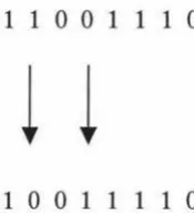
2.3.3 Bit Mutation

The bit mutation operation is applied to a single individual within the population. The

individual is again selected based on the fitness. Individuals with higher fitness have higher

chance of being selected and individuals with lower fitness have lower chance of being

selected. Mutation occurs on one or more bits. The mutation operation toggles a bit in the

1 1 0 0

1 1 0

l l

0 0 1 1

0

Figure 2.3.1. Mutation operation changes bit value.

The mutation operation extends the search space with new points.

2.4 Parameter Selection

Parameter setting is important because it determines the run time behaviour of the

algorithm. The primary parameters for controlling a genetic algorithm are the population

size and the maximum number of generations to be run. Secondary parameters, such as

reproduction probability, crossover probability and mutation probability are also important.

In addition, some parameters such as the selection method have to be determined.

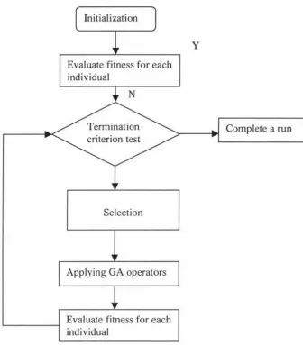
2.5 Structure Of Genetic Algorithm

Initialization

Evaluate fitness for each individual

Selection

Applying GA operators

Evaluate fitness for each individual

Figure 2.5.1. The flow chart of conventional GA.

y

Complete a run

The first step in performing a GA is to randomly produce an initial generation. This is

called initialisation. The number of individuals within this generation is determined by the

value of the population size. After initialisation, all individuals in the population have to be

value satisfies the requirement of the system, the GA procession terminates. Another

termination criteria may be the maximum number of generations. Once this value is

reached the system is terminated.

The next step is selection. This determines the objects that genetic operators will apply to.

Reproduction and mutation operate on a single individual and crossover operates on two

parents. After applying genetic operators to individuals, new individuals will be generated

and they will be put in the next generation. Fitness evaluation should be done after any step

evolving genetic operators.

The best solution and desired solutions should be recorded at the termination stage.

2.6 An Example

Now let us consider an example of applying genetic algorithms to solve a problem. The

problem is to find the maximum value of the sine curve. The formula we illustrate here is:

f (x)

=

+

The x value varies between 0 and 15. Step length is set to 1. This is an optimisation

problem.

To solve this problem we have to provide a concrete implementation of the steps stated

above. The most commonly used representation language for the basic genetic algorithm is

a fixed length binary string. We will also follow this scheme in this example. Since our step

length is 1, and the total number of sample points is 16, it is possible to represent the

the possible solution must be included in the scheme. If the precision required is higher, the

number of bits in the string must be increased to satisfy this requirement. In other problem

domains, different lengths of string and different coding alphabets may be adopted. It is

sometimes difficult to determine the representation scheme.

To design the fitness function, we first have to describe the error between the target value

and the calculation value. Since the function has a value between 0 and 2, we can calculate

the error as:

error= 2- (sin(x;r /8) + 1)

This makes the error value always positive.

It is quite straightforward to design the fitness function now:

fitness

=

The fitness value will be 1 when error is 0. If we find the maximum value of the curve, we

wi 11 have the fitness value 1.

Population size is set to 5. This is sufficient for such a trivial example. Maximum

generation size is 10. If the ideal result is not found within 10 generations, we terminate the

program and run it again.

We assume that we have no a-priori knowledge about this problem. Before starting the

generation loop, we initialise the individuals in the population randomly. In one run, we

Generation 1: Generation 2:

String Fitness String Fitness

1101 0.09 0000 0.17

1101 0.09 1010 0.10

1101 0.09 1101 0.09

0000 0.17 1101 0.09

1100 0.09 1010 0.10

Total Fitness: 0.53 Total Fitness: 0.55

Generation 3: Generation: 4

String Fitness String Fitness

1000 0.17 0100 1.00

0101 0.72 1011 0.09

1010 0.10 0101 0.72

1010 0.10 0101 0.72

0000 0.17 1010 0.10

Total fitness: 1.26 Total Fitness: 2.63

The total fitness value in the first generation is 0.53. No genetic operator is applied to the

individuals in this generation.

After initialisation, genetic operators will be applied to the individuals. The genetic

is simulated in selecting the genetic operator object. The individuals with higher fitness

values have high chances of being selected. In practice, a very common approach called

roulette wheel selection is used to perform the selection. This approach has the advantage

of being simple to implement. An individual's probability for selection is given by:

pk (selection )

fitness

L

fitness

i=l

Here, N is the population size. The higher the fitness value of a particular individual, the

higher is its probability of being selected for the next generation. This can be illustrated by

using a roulette wheel, each fitness value occupies a part of the wheel. The bigger the

fitness value, the larger part it occupies. A random point is selected from the wheel. A

larger part has the higher probability to be selected. In implementation, we calculate the

total fitness. A random value is selected between 0 and the total fitness.

For generation 1 in our example, we add up the fitness from individual 1 to individual 5.

The partial sum is marked on the line. After a random point is selected, we observe that the

left side of the random point is just the sum of the fitness from individual 1 to the random

point. If we keep adding the fitness starting at individual 1, if the sum is greater than or

equal to the random value, we select that individual. Note that crossover requires two

parents, these are selected separately. These two parents may be the same individual.

Reproduction is performed by selecting an individual and copying it into the new

population. Note that the new individual may not sit at the same position as the individual

in the old generation. Fitness value does not need to be re-evaluated. A copy will reduce the

calculation effort. Crossover is performed between two parents. A cross point is selected

randomly between the second bit to the last bit. Mutation is performed by randomly

toggling one bit in the selected individual. It produces one child, which is placed in the new

population. The choice of which genetic operator to use is controlled by a probability. A

weight between the three operators can be distributed.

There are two termination criterions in this example. One is the maximum generation and

another one is the best fitness reached. The running result shows four generations. We can

3. A Short Introduction To Genetic Programming

Genetic programming as a field was introduced by John Koza[25] in 1992. Genetic

programming is an attempt to answer the question: "can computers solve problems without

being explicitly programmed?" That is, how can computers be made to do what needs to be

done without programming. GP is based upon Holland's genetic algorithm [16]. The

difference between GP and Holland's GA is that GP gives the solution to the problem in

abstract syntax trees instead of a fixed - length bit string. The solution to the problem is

evolved using a set of examples and the training process is a calculation of the distance

between the solution and the desired target.

GP runs with an initial process. In this process, a population is created. Each individual represents an abstract syntax tree which is made up with a series of functions and terminals.

The designer has to give the proper function set and terminal set so that the problem can be

solved. A fitness value is set up to determine how good an individual is at solving the

problem. The fitness value is designed to simulate the ability of surviving. In computer programming, an abstract syntax tree should be a computable expression. Since it is possible to calculate an abstract syntax tree for each set of input data, the fitness function

can be designed to determine the fitness value based on the result of the abstract syntax

tree. Training data is usually a set of input output data pairs. The fitness value should reflect

the strong level of the tree toward all of the training set. In practice, a distance is used to

represent how fit the tree is by comparing the output data of the training set and the result

After initializing the population, the GP mechanism will take over and search the problem

space. A tree can be created from the function set and terminal set while the fitness function

determines how close the tree is to the problem specification. During running of the GP,

new individuals are produced continually and a fitness value for an individual is attached to

itself. The commonly used GP operators are reproduction, crossover and mutation.

Reproduction is a method that copies an individual in the population and places it into the

new population. Reproduction copies the abstract syntax tree as well as all the information

attached to the tree, including the fitness value. The fitness value is used to determine the

chance of reproduction. Reproduction results in more useful abstract syntax trees appearing

in the population.

The crossover operation is a sexual operator: it takes two parental programs selected based

on fitness. The parental programs in genetic programming are typically of different sizes

and shapes. The offspring programs are composed of sub-expressions from their parents.

Often a GP program has a maximum depth to limit the computing time and ensure any

program is bounded by the maximum program size. If the newly generated program size is

longer than the maximum size, it is necessary to select another node from the parental

programs or to reproduce the parent program. Crossover provides a mechanism to explore

the search space by creating a new program that combines advantages of parents with high

Mutation operates on one program, from this one or more nodes is selected to be modified.

The selected node is replaced by a randomly generated new node. The newly generated

individual should be bound to the maximum program length. After mutation, the fitness of

the program is evaluated and is placed in to the population. The mutation operator helps to

avoid local optima in the search space.

During the run, GP operators operate with a given probability. Individuals or parents are

selected based on Darwinian evolution. Obviously, population members with high fitness

values should have a high chance of survival and have a high chance of helping form the

next generation than those with a low fitness value. In genetic programming, parents are

selected through a use of a stochastic selection scheme. Individuals with a higher fitness

value have a higher chance of being selected as a parent than those with low fitness values.

The fitness value will drive the population moving from one generation to next, and like

natural selection, only the strong individuals can survive. The average fitness of the next

generation will be higher than the previous generation. In such a way, the population can

evolve over time.

Each individual in the population during the search process represents a point in the search

space. The entire population makes up the search space. Using the fitness, the exploring

process moves toward the highest point which implies the desired solution to the problem.

When the generation reaches the highest point in the search space, a termination criterion

There are five major steps in applying genetic programming to solve a problem.

1. determine the set of terminals.

2. determine the set of functions.

3. determine the fitness function.

4. determine the parameters and variables for controlling the run.

5. determine the method of designating a result and the criterion for termination of a

run.

Step one determines the terminal set which may be viewed as an input to a computer

program. Step two determines the function set which is a mathematical operation or some

operational functions.

The terminal set and function set make up the abstract syntax tree which makes exploring

the problem possible. The last three steps correspond to the steps for a conventional genetic

algorithm.

Genetic Algorithms are stochastic search techniques introduced by Holland[16] which takes

the Darwinian idea of natural selection, or "survival of the fittest", and applies it to digital

computation. The essence of the algorithm is that a population of individuals is evolved

over generations. The individuals that are more fit have more survival chance than others.

A Genetic Algorithm starts with an initial 'population of trial solutions to a problem'. The

next problem is to determine the sort of representation that GA should manipulate. The

traditional simple GA, as defined by Holland represents the problem's data as

units into binary strings, where each bit corresponds to a single gene. A group of such binary strings is the population, with each individual of the population referring to a single

possible solution to the particular problem. The population of the first generation is

generated randomly and the genetic operators will be applied to the individuals in the

population. As in nature, after certain generations, the average fitness of the population will

be stronger.

The interaction of the genetic operators and the stochastic selection based on survival of the

fittest individual results in an exploration of the search space. Natural selection and the

reproduction operator provide the hill climbing pressure to improve the fitness of the

overall population. Reproduction provides the means of search space exploration by

cloning abstract syntax trees with high fitness. Mutation maintains the diversity required to

avoid local optima in the search space. Since fitness of individual abstract syntax trees is

based upon the input output specification of the desired program, the result of the search is

an abstract syntax tree which will satisfy the desired behavior or closely approximates it.

3.1 The Standard GP

Koza(1989, 1992) describes a genetic programming system using Lisp S-expressions. In his

foundation work, he uses a tree-based representation as the genetic algorithm framework.

Some basic genetic operators for genetic programming such as mutation and crossover

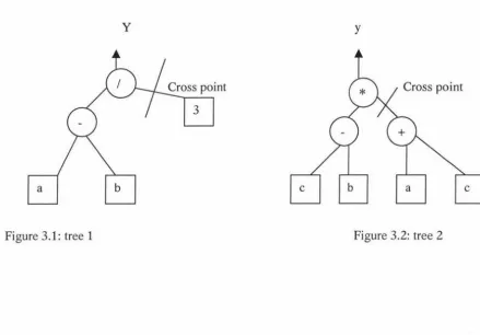
were defined. Consider the problem with two variables a and b, output variable y is

represented in the form:

This expression may be represented as a tree structure in figure 3.1.

y _y

Figure 3.1: tree 1 Figure 3.2: tree 2

If we have another tree structure, in figure 3.2, tree2, crossover may be applied to these

trees. The cross points are as shown on the figures above. Two cross fragments are shown

as follow.

3

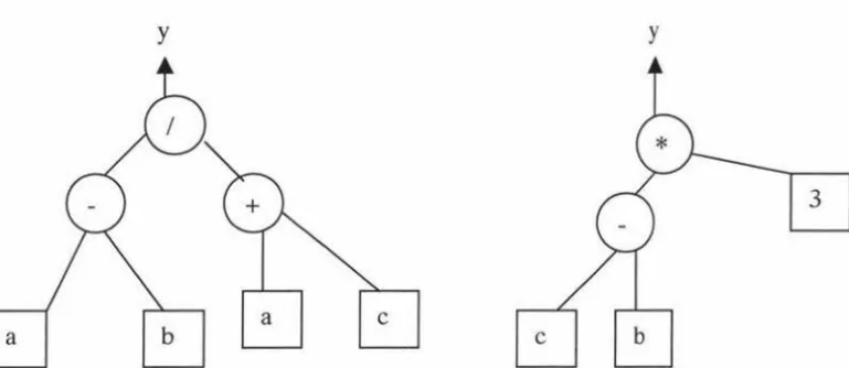
The two cross fragments exchanged position after the crossover operator is applied. The

resulting offspring are as follows:

y y

Figure 3.5: Tree 1 after crossover Figure 3.6: Tree 2 after crossover

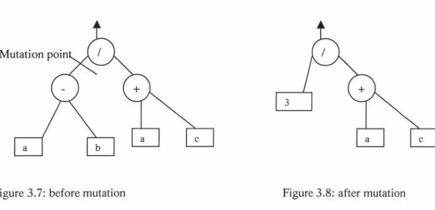
In Koza's Lisp based GP, some constraints are applied to the tree structure. Two

parameters, the depth and number of nodes are often defined. The mutation operation

begins by selecting a mutation point. The mutation point is selected as a function or

terminal. The mutation operation removes the selected point or below the selected point and

3

Figure 3.7: before mutation Figure 3.8: after mutation

One of the properties of genetic programming is that the tree may be generated randomly.

A function may call other functions or be called by other functions. The closure property

must be satisfied. Kosa defines the closure property as each of the functions in the function

set be able to accept, as its arguments, any value and data type that may possibly be

returned by any function or be taken by any terminal [25].

For example, a Boolean operation may only take Boolean values such as True or False but

not number values. Therefore it must be ensured that every function within the tree

structure is provided with suitable arguments. This must be the case for every possible

combination of functions and terminals that the system might encounter during

initialisation of a tree. The closure condition must also be satisfied when applying genetic

operations such as mutation and crossover.

Providing a function argument with the wrong type is not the only example of violating the

division by zero, Koza [25] defines a function known as protected division. When a

function, which performs protected division, encounters an argument of zero for the

divisor, it produces a string ':undefined' for its output. All other functions within the

function set have to be changed so that they can deal with this result. Other examples of

violated closure condition are square root and logarithm of a negative number.

3.2 Differences Between Genetic Algorithm And Genetic Programming

Angeline [2] compares and contrasts genetic programming with genetic algorithms. In this

analysis he discusses three differences between genetic algorithm and genetic

programming: (a) the representation of genotypes, (b) the complexity of interpretation, and

(c) the use of syntax preserving crossover.

Genetic algorithms generally use a genotype, which is a fixed-length string of characters

from a low cardinality alphabet. Genetic programming uses a variable sized tree

representation for its genotype. It is claimed that the use of this representation makes genetic programming more powerful than genetic algorithms. Angeline concludes that in

practice the representations are equivalent. In most genetic programming systems there is a

maximum size to the trees that can be generated. In addition the functions used in genetic programming have fixed known branching factors. Under these constraints, the trees used

in genetic programming can easily be represented as variable length strings with the union

of the terminal and non-terminal symbol sets used as the alphabet. Given this equivalence

of representations, genetic programming can be viewed as a genetic algorithm that operates

The second area where it is claimed that genetic algorithms differ from genetic

programming is in the interpretation of the representation as a genotype. The strings used in

genetic algorithms are generally interpreted using a positional encoding where the meaning

of an element is based on both its symbol and its position in the string. Conversely, in

genetic programming the encoding has no positional component in its interpretation. A

function symbol has the same meaning no matter where it may appear in the tree. This

looks to be a difference, but it is only a difference in standard practice. There is no

theoretical reason why a genetic algorithm could not interpret the characters in its

string-based representation without regard to their position.

The final area in which there is a potential difference between genetic algorithms and

genetic programming is in the operators used in the two types of systems. In genetic

algorithms the crossover and mutation operators are fully general and have no component

which considers the interpretation of the strings. In contrast, the crossover and mutation

operators in genetic programming are carefully defined to produce syntactically correct

trees after the completion of the operation. The operators know that they are manipulating

trees and build their output so that it can always be manipulated by the interpretation

function. Angeline concludes that the use of syntax preserving operations in genetic

programming is the only real theoretical difference between genetic algorithms and genetic

4. Related Work

In Koza [25](10.13), image compression is mentioned and he successfully evolves a model

to compress a 30X30 bitmap image with a good solution in standard GP. Because of the

vast computation necessary, only a small image was tested in Koza's work.

In Koza and other standard GP systems, an S-expression is evolved and evaluated. Most of

the time is spent on evaluating each S-expression. To increase the speed of evaluating each

S-expression, Fukunaga et al [12] developed a compiler for an efficient GP system. The

Gnome compiler translates each S-expression into SPARC machine language codes before

evaluating it. Simple arithmetic operators can be executed with a single instruction at the

hardware level instead of many recursive function calls in standard LISP S-expression. In

one paper [12], a predictive coder is evolved that can be used for multi-level

compression(e.g. a Huffman coder). They worked on a 64X64 image and this proved much

faster than the standard GP system.

Predictive coding is an image compression technique, which uses a compact model of an

image to predict pixel values of an image based on the values of neighbouring pixels. A

model of an image is a function, such as PredictedModel (neighbour Value), which

computes the pixel value at coordinate ( x, y) of an image. The neighbour value is known to

the predicted pixel. Linear predicted coding is a simple case of predictive coding in which

the model simply takes a weighted average of the neighbouring value. Nonlinear predicted

coding assigns arbitrarily complex functions to the model. The algorithm of predicted

Encoder (Model, Image)

for x=O to xmax

for y= 0 to ymax

Error [x, y] = Image[x, y]

-PredictedModel(neighbourValue)

Decoder(Model)

for x = 0 to xmax

for y = 0 to ymax

Image[x, y] = PredictedModel(neighbourValue)

+ Error[x, y]

Applying a model to an image results in an error between the original image pixel value

and the predicted value. The error can be compressed using standard compression methods

such as Huffman coding. Applying the model to the error can recover the original image.

Nordin and Bnazhaf [34] use the idea of programmatic compression to compress sound and

image data. They use a chunking method to process an image that makes the system easier

to converge to an expected solution. The picture was divided into 8X8 or 16X16 pixel

blocks. Chunking involves two systems. The first treats all the fitness cases at the same

time. The second applies programmatic compression to equally sized sub-sets of the fitness

cases and evolves a solution to each of them. Programmatic compression works on a

Compiling GP system(CGPS) that ensures a high speed evaluation of each fitness case.

They also claimed that it is the first time to compress a real full size image(256X256)

The basic idea of programmatic compression is that any system, which evolves programs or

algorithms for generating data, can be viewed as a data compression system. The data that

should be compressed are presented to the genetic programming system as fitness cases for

symbolic regression. After choosing a function set that facilitates an accurate reproduction

of the uncompressed data, the system then tries to evolve an individual program that, to a

certain degree of precision, outputs the uncompressed data. If the evolved program solution

5. Implementation Consideration

This chapter contains a discussion of many different implementation techniques that may

be applied to a genetic programming system.

5.1 Representation

The parse tree representation was first used in Cramer(1985). In this representation,

functions and variables are expressed as numbers instead of explicit symbols and stored in a

fixed - length string. The numbers can be matched to functions according to a lookup table.

For instance, an encoded program could have the form (4 (1 3) (2 1 (2 2 (0 3))))), where the

parentheses denote a complete statement. The lookup table could have the following form.

Number Function Meaning

0 : INC VAR Increment [VAR]

1 :ZERO VAR Set [VAR] =0

2 :LOOP VAR FUNC Execute [FUNC] [VAR] times

3 :SET V ARl V AR2 [VAR1]=[VAR2]

4 :BLOCK FUNCl FUNC2 Execute [FUNCl] then [FUNC2]

The program above can be represented as:

(:BLOCK (:ZERO V3) (:LOOP Vl (:LOOP V2 (:INC V3))))

Note that in Cramer's tree - based language structure, a subtree argument does not return a

In Koza's parse tree representation, the subtree arguments in genetic programming return

values to their calling statement. A function can call other functions recursively and can be

called by other functions in the same way. A typical parse tree is showed in figure 5.1.1. In

such a representation, a maximum length restriction is imposed on the evolved program.

Without such a restriction, the dynamically generated program may increase in size

uncontrolled, eventually swamping the computer's available resource. There are two

common restrictions. One is the depth limitation, which restricts the size of evolving parse

trees based on a user-defined maximal depth parameter. Another one is node limitation,

which limits the total number of nodes available for an individual parse tree. In practice,

node limitation is more used. This is because of its easy implementation and the fact that it

imposes fewer limitations on the structural organisation of the evolving program.

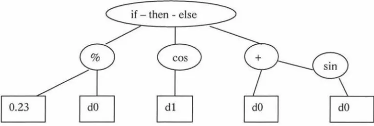
In a parse tree representation, the primitive language definition is crucial for the solution to

the particular problem. The solution must be bounded in the definition of the primitive

language. Koza addresses this as the sufficiency property. Sometimes the representation

primitive language may be taken from the programming language, but typically it is

tailored by carefully consideration of domain-specific knowledge. For instance, in Koza's

artificial ant problem[25], the primitive language includes elements such as move, right,

0.23

Figure 5.1.1: a typical parse tree

It is sometimes necessary to insert a constant into an evolved program. The most common way of doing this is to use a symbol to represent a constant. The constant is then usually an element of the terminal set. When evaluating an individual that contains a symbol, rather than evaluate the symbol directly, the symbol is replaced by a relative constant. For instance, in the terminal set T={ CONl, dO, dl}, dO and dl represent two input parameters and CONl represents a constant. When CONl is evaluated in the evolved parse tree, a relative constant (say 2.34) is inserted and evaluated.

5.1.1 Automatically Defined Functions

In standard genetic programming, the function set generally contains primitive functions that can be defined before the program runs. For a simple problem, this may be sufficient to solving the problem. However, in some cases, it may be difficult for a solution to be

automatically defined functions. ADFs are evolvable functions (subroutines) within an evolving genetic program, which the main routine of the program can call [26].

ARGl

I

s

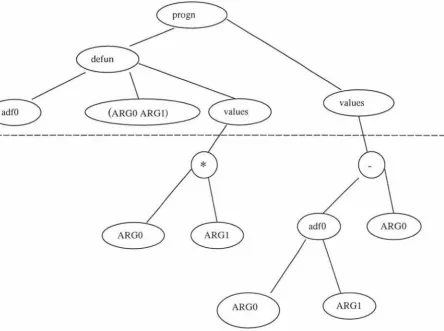
Figure 5.1.2 A program containing an ADF.

across the entire program system. The function defined by the function defining branch of

an individual is available for use by the result producing branch of that individual. Calling

automatically defined functions is not predetermined, instead, it is determined by the

evolutionary process.

Figure 5.1.2 shows the tree structure of an example program. This figure is divided into two

sections, those portions of the tree above the dashed line and those portions of the tree

below the dashed line. The portions of the tree above the dashed line represents the fixed

structure of the procedure, which must be maintained in every individual in the population.

The portions of the tree below the dashed line represent the parts of the procedure that can

be evolved to solve the problem.

In order to use automatically defined function, two considerations that are different from

standard genetic programming must be taken into count. First, the procedure that creates

the initial population must be modified to generate individuals with the required fixed

structure. Second, the genetic operators must be modified to maintain the fixed structure of

the tree and to operate only on the modifiable areas within a tree.

To avoid the possibility of infinite recursion between the defined procedures, the genetic

material which may be used in each evolvable branch of the tree is separately defined so

that procedures defined within the main procedure may not call each other, but may only be

Koza gives the functions that an automatically defined function can perform.

o Perform a calculation similar to that which a human programmer might use

o Perform a calculation unlike anything a human programmer would ever use

o Redundantly define a function that is equivalent to a primitive function that is

already present in the function set of the problem

o Ignore some of its dummy variables

o Be entirely ignored by every potential calling branch

o Define a constant value

o Return a value identical to one of the dummy variable(so that the automatically defined function redundantly defines a terminal that is already present in the

terminal set of the problem

o Call another automatically defined function with a subset of or a permutation of its dummy variables

Several sets of experiments have been performed to compare the performance of genetic

programming systems that use automatically defined functions with those that do not [26].

The results of these experiments show that the use of automatically defined functions

increases the power of a genetic programming system in terms of the difficulty of problems

that it can solve. The technique also improves the speed at which solutions can be obtained

(measured in terms of the number of individuals searched) for all but the most trivial of

compact solutions than those found without the technique. The reuse in the main routine of

the subroutines evolved by the system allow for this reduction in program size.

5.2 Selection

Selection in genetic algorithms is the process of choosing which individuals in the

population will be allowed to propagate their genetic material through application of a

genetic operator. The selection operator does not create any new solutions, instead it selects

relatively good solutions from a population. The takeover time is defined as the speed at

which the best solution in the initial population would occupy the complete population by

repeated application of the selection operator alone[9]. Selective pressure is the

phenomenon that highly fit individuals have a high probability of being selected. If the

takeover time of a selection operator is large, the selective pressure of the operator is small.

If the selection operator has a large selective pressure, the population loses diversity

quickly and may converge to a local optimum. If the selection operator has a small selective

pressure, the population will converge slowly and reduce the ability to search the entire

space. A different selection operator applies a different selection pressure to the population.

The sections below will discuss a number of common used selection operators.

5.2.1 Proportional Selection

Proportional selection assigns to each individual a reproductive probability that is

proportional to the individual's relative fitness. Proportional selection was first introduced

algorithms. In this scheme, the probability of selection of a single individual i in the

population is characterized by the equation below:

f

p,. (selection)

=

I

1

Here

f

function to a non negative real value, which is proportional to the fitness value of

individuals. N is the population size.

The fitness mapping function is crucial to proportional selection. An individual with the

same fitness value will have a different selection probability when different mapping

functions are used. For example, consider two individuals with fitness 1 and 2 respectively,

the second individual has twice the selection probability of the first one. But if the mapping

function adds 1 to all individuals, the fitness of first individual will change to 2 and the

second one will change to 3. In this case, the second individual has only 1.5 times the

selection probability of the first one.

In some genetic algorithms it is necessary to select an unreasonable individual to replace

some individual in the population in order to increase the diversity. In this case, a possible

method is to give a high reward to the poor individuals. This is the inverse proportional

selection.

f

p,. (selection)

=

I

1

In this case, the mapping function has the same form as the normal mapping function but

The scatter of fitness value may lead the population toward premature convergence. At the

beginning of a run, an individual with a high fitness value will be preferred and produce

more offspring. The similar structure of the string will occupy most of population. This will

cause the search to stop at a local optimum.

5.2.2 Windowing

Windowing is a method used to avoid a local optimum by evaluating the fitness function as

a time-varying transformation. It can be expressed as:

<I>

=

f

(fitness) -

f3

(t)

Here <I> 1 is the windowing fitness mapping function.

f

mapping function that maps the raw fitness value to a non negative value. (3(t) represents

the worst value seen in the last few generations. The number of generations used is given

by the windowing size w. w is typically between 2 and 10.

Since (3(t) normally improves over time. In the later stages of search, windowing provides

great selection pressure. However, poorly performing individuals may occasionally arise

5.2.3 Sigma Scaling

Sigma scaling is based on the distribution of fitness values over the entire current

population. When windowing scaling is applied, one problem is that particularly poor

individuals may push the baseline very low. Sigma scaling is defined as follows:

<I> . =

{f (fitness;)

-

(/

c a

I

0

If

f

is applied.

f

a

deviation of the objective values in the current population. c is a constant (e.g. c=2).

The sigma scaling method relies on the average fitness of the population, this may lead the

premature convergence to a super fit individual.

5.2.4 Tournament Selection

In tournament selection, a group of q individuals is randomly chosen from the population.

They may be drawn from the population with or without replacement. This group takes part

in a tournament. That is, a winning individual is determined depending on its fitness value.

Tournament selections are held with a group of size q, called the tournament size. q is

usually between 2 and 10.

Tournament selection can be implemented very efficiently because no sorting over the

entire population is required. Tournament selection also has the advantage of simple

selection. However, tournament selection only relies on the fitness of the tournament group,

no scaling technique is needed. Tournament selection is also suitable for a parallel

evolutionary scheme. Since the tournament group is a local parameter rather than from the

global population. Evaluations are performed on the local tournament group.

Selection pressure is modified in tournament selection by varying the tournament size.

Tournament size is equal to 1 corresponds to no selection at all. It is just a random selection

from the population. As the tournament size increase it becomes more likely that the fittest

individual will be chosen. For many applications in genetic programming, tournament size

take the range between 6 to 10.

One interesting variant of tournament selection is the notion of competitive fitness, which is

used to evolve game playing programs [11]. In games, which are non-trivial, it is extremely

difficult to generate a correct, heuristic solution for specifying fitness. Competitive fitness

requires the members of the tournament to actually play against each other in order to

determine the fittest individual. Fitness is determined with the record of each individual in

the competition. The method has three advantages. First, it does not require the user to have

the detailed domain knowledge required to write the complete and correct fitness function.

Second, a well defined fitness function does not provide for good differentiation between

poorly fit individuals during the initial generations of the algorithm. Competitive fitness

notes these distinctions by computing fitness in a way that improves fitness over time.

Finally, since an individual may encounter many different strategies in a tournament,

competitive fitness rewards those individuals that are able to compete well against a

In those cases where an inverse selection scheme is required to determine which member of

a population is to be replaced, inverse tournament selection can be used. In this scheme, the individual with the worst fitness in the tournament is selected for replacement.

5.2.5 Rank - Based Selection

Hancook [15) summarised the different ranking selection that may be applied in practice.

The basic idea is to sort the population from best to worst in the current generation, and then assign a reproductive or survival probability to each individual that depends on the

rank ordering of the individuals. Linear ranking, non-linear ranking, (µ, A.) selection and

(µ+A.) selection are methods of rank-based selection.

5.2.6 Linear Ranking

The most common form of ranking is linear ranking. In this scheme, the assignment

function is a linear function that assigns individuals a fitness value which depends on the position of individuals in the queue instead of the actual fitness. If the index of the

individual with highest fitness is µ-1 and the index of the individual with worst fitness is zero, the selection probability for individual i is defined as follows:

<I>

.

a

+

[rank

(xµ

-1)

J

(J3

a

where i is the index of individuals. arank is the number of offspring allocated to the worst

individual. f3rank is the expected number of offspring to be allocated to the best individual

during each generation. µis the population size. The sum of the selection probability can be

calculated:

µ-I 1

~<I>

;

Z

The total probability is 1. Thus, 1:::;; /3rant :::;; 2, and a rant =2-/3rant . If /3ran1c is set to 2, the

worst string has no chance of reproduction. In principle, f3rank could be increased beyond 2

to achieve higher selection pressures, but then several of the worst strings would be given negative fitness values. These could be truncated to zero, but then the remaining fitness values would need rescaling to give the correct total number of offspring.

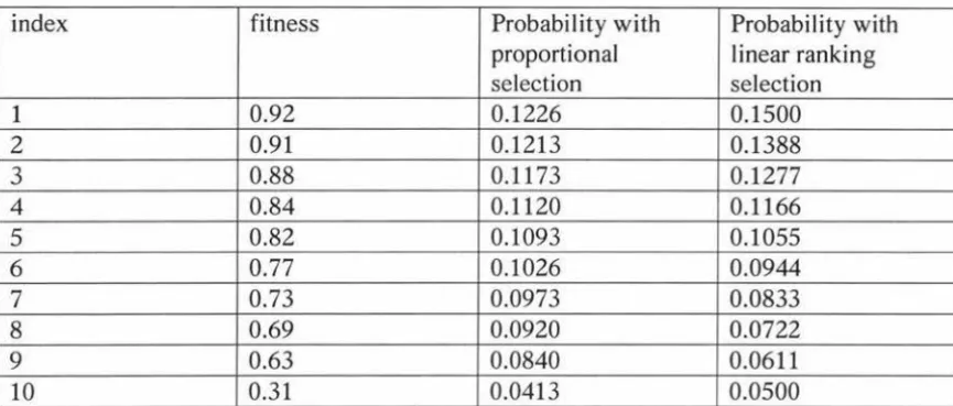
As an example, consider the population whose fitness is presented in table 5.2.1. The

proportional selection probability is computed by dividing each fitness value by the sum of the fitness values. For linear ranking the population is sorted in decreasing order. The

probability of each individual is computed using the formula given above with µ=10, and

index fitness Probability with Probability with proportional linear ranking selection selection

1 0.92 0.1226 0.1500

2 0.91 0.1213 0.1388

3 0.88 0.1173 0.1277

4 0.84 0.1120 0.1166

5 0.82 0.1093 0.1055

6 0.77 0.1026 0.0944

7 0.73 0.0973 0.0833

8 0.69 0.0920 0.0722

9 0.63 0.0840 0.0611

10 0.31 0.0413 0.0500

Table 5.2.1: comparison of proportional selection and linear ranking selection

Linear ranking provides increased selection pressure over proportional selection schemes.

This is due to the weakness of proportional selection schemes in the latter portions of their

search. As the average fitness of the population in a proportional selection scheme

approaches the global optimum, the deviation between fitness values decreases. This drives

selection probability of each member of the population in the limit to

fµ.

proportional schemes fail to reward individuals with marginally better fitness values in the

final stages of the search. Linear ranking provides a fixed advantage throughout the entire

search process to those individuals with better fitness, thus capitalizing on minute

differences in fitness in the later stages of the search process. Empirical experiments show

that linear ranking improves selection pressure up to five orders of magnitude over

5.2. 7 Exponential Ranking

Another ranking-based selection is exponential ranking. It is similar to linear ranking in that it uses an assignment function to determine the numbers of offspring. It is different from linear ranking in that the assignment function is not a linear function. The selection probabilities might be proportional to the square of the rank:

a

+

[rank

2

J

((3

_a)

<I> i

= _;;:;___

/

_

-c

where c

=

-%{µ

-

l

)

meaning as in linear ranking and usually, 0 <a<

/3

.

13

change the selection pressure. Increasing

13

a

pressure and vice versa.

5.2.8 (µ, A.) And (µ + A,) Selection

In (µ, A.) selection, each individual in the population is allowed to reproduce k offspring in

the next generation. A.=k µ, where µ is the best individuals selected in the current

generation, and k is the expected number of the offspring of µ in the next generation. Fork > 1, the best individuals will produce many offspring while some poor performing

In (µ +.A) selection, the individuals that are going to be parents are selected from the union

of the best µ individuals from the old generation and best .A individuals from offspring. The

(µ+.A) method always retains the best individuals unless they are replaced by superior

individuals.

In these two methods, the best individuals always win against competitors. Selection

pressure is high and takeover time is very low.

5.3 Genetic Search Operator

In evolutionary computing, an individual in the population represents a solution to the particular problem. A fitness value is adopted to measure how good the individual is. As evolving progresses, a new individual is generated by selecting one or more fit individuals

and applying a genetic operator to the selected individuals. The mutation operator creates a

new individual by changing one individual while the crossover type operator generates a

new individual by combine some parts of two individuals.

5.3.1 Mutation

Mutation is one of the commonly used genetic operators in evolutionary computing. In

mutation, one allele of a gene is randomly replaced by another to yield a new structure [16).

Mutation has the benefit of maintaining diversity in the population to avoid premature

convergence. In a fixed-length genetic algorithm, mutation is necessary because at the

another. As evolution is carried out, the population may retain similar genetic material, the

desired genetic material may not exist in the population, mutation provides a mechanism to

generate a new allele and put it into the population.

Koza [25] describes a mutation operation in which an entire subtree of the selected tree's

copy is replaced with a randomly generated subtree. The depth of the subtree is controlled

on a similar way to the random creation of the initial population. However, Koza argues

that mutation is not important in genetic programming.

First, in genetic programming, particular functions and terminals are not associated with

fixed positions in a fixed structure. Moreover, when genetic programming is used, there are

usually considerably fewer functions and terminals for a given problem than there are

positions in the chromosome in the conventional genetic algorithm.

Second, in genetic programming, whenever the two crossover points in the two parents

happen to both be endpoints of trees, the crossover operation operates in a manner very

similar to point mutation. Thus, to the extent that point mutation may be useful, the

crossover operation already provides it.

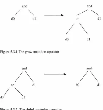
Angeline[l] defines four distinct forms of mutation for parse trees. The grow mutation

operator randomly selects a leaf from the tree and replaces it with a randomly generated

new subtree. The shrink mutation operator selects an internal node from the tree and

replaces the subtree below it with a randomly generated leaf node. The switch mutation

operator selects an internal node from the parse tree and reorders its argument subtrees. The

cycle mutation operator selects a random node and replaces it with a new node of the same

selected , then it is replaced by a function primitive that takes an equivalent number of

arguments. The four mutation forms are illustrated in figures 5.3.1- 5.3.4.

and and

/

""

dO

dl

dl

/ \

dO

dl

Figure 5.3.1 The grow mutation operator

and and

/ \

/ \

or

dl

dO

dl

/~

dO dl

if

/ii~

d2 or ana

/I~

and or d2

I

1\

/I \

dO

dO

Figure 5.3.3 The switch mutation operator

if if

/I~

/I~

and or d2 and and d2

\

_II

\

dl d2

dO

Figure 5.3.4 The cycle mutation operator

5.3.2 Crossover

string locations are chosen as breakpoints (crossover points) delineating the string segments

to exchange. Finally, parent string segments are exchanged and then combined to produce

two resultant 'offspring' individuals. The method used in Koza [25] is one point crossover.

As the name suggests, only one crossover point is selected in parent individuals and the

subtree below the crossover point is swapped between two parents. Koza [24] suggested

that a selection bias should be applied to the parent's selection so that in most cases, a node

is selected as a crossover point instead of leaf. This can balance the depth of nodes in the

tree.

Takuya et al [20] introduced a depth - dependent crossover. In standard crossover, a node

is selected randomly regardless of its depth. It has an influence on the resultant structure in

two ways. First, the operator swaps larger parts of subtrees for shallower nodes. This leads

to the propagation of larger parts of useful subtrees to the entire population. Second, the

operator encapsulates a larger part of a tree, so that substructures for shallower nodes are

protected from the destructive crossover. This random selection may not work well for the

effective recombination or for the accumulation of building blocks. For depth-dependent

crossover, a node is selected depending on its depth. The algorithm for depth - dependent

crossover is:

Step 1: Given a tree, determine the depth d for applying the depth - dependent

crossover.

Step 2: Select randomly a node of which depth is equal to din Step 1.

A bias is applied to the selection of depth d so that the node is closer to the root. Takuya claimed that this improves the crossover performance and accumulates building blocks. As the generated programs become large, depth-dependent crossover does not work

efficiently. This can be overcome by non-destructive depth-dependent crossover, in which each offspring is kept only if its fitness is better than that of its parent. In some

experiments, non-destructive crossover generated smaller programs in Takuya's work.

Poli and Langdon[37] introduced a variation of crossover called one point crossover, which works by selecting a common crossover point in the parent programs and then swapping the corresponding subtrees like standard crossover. The crossover locations are chosen only from those parts where both parents have the same shape. A study [38] reports that one point crossover is valid and improves the performance of standard crossover significantly.

Uniform crossover [35] takes the same name as in genetic algorithms but has a different operation. In GA uniform crossover, the positions of parent strings are denoted as 0 or 1,

offspring 1 copies the elements directly from parent 1 in those bit position marked by a 1.

are both copied. Interior nodes are selected for crossover with some probability. Non

interior nodes within the common region can also be crossed, but the nodes and their

subtrees are swapped. Nodes outside the common region are not considered. As reported,

using this representation, performance on the even-6-parity problem is improved by three

orders of magnitude compared with standard genetic programming.

D'haeseleer [10] describes two variations on crossover. The first variation is called strong

context preserving crossover. In this method, subtree swapping is limited to those subtrees

which are in exactly the same position in both parent trees. This is accomplished by first

uniquely naming each node in both trees as a tuple of n coordinates T

=

which specify the path from the root of the tree to the subtree root. Where n is the depth

from the tree root to the subtree root and each bi represents its branch, in left to right order.

If a node is identified in parent 1 with a matching node in parent 2, the nodes and their

subtree are swapped. This is similar to GP uniform crossover except for the interior region.

The second variation presented is called weak context preserving crossover. In this

variation, the same node naming scheme is used. The subtree selected from the first parent

is taken from among the nodes in which there is a matching node in the second tree. The

subtree selected from the second parent is a random subtree of the node that matches the

name of the first parent's subtree. This modification maintains a certain sense of lexical

locality and overcoming the problem with good genetic material being unable to migrate