Machine learning for geological mapping : algorithms and applications

M

APPING

: A

LGORITHMS AND

A

PPLICATIONS

MATTHEW

J. CRACKNELL

BSc (Hons)

ARC Centre of Excellence in Ore Deposits (CODES)

School of Physical Sciences (Earth Sciences)

Submitted in fulfilment of the requirements for the degree of

Doctor of Philosophy

Did you ever fly a kite in bed?

Did you ever walk with ten cats on your head? Did you ever milk this kind of cow?

Well, we can do it. We know how. If you never did you should. These things are fun and fun is good.

D

ECLARATION OF ORIGINALITY

This thesis contains no material which has been accepted for a degree or diploma by the University or any other institution, except by way of background information and duly acknowledged in the thesis, and to the best of my knowledge and belief no material previously published or written by another person except where due acknowledgement is made in the text of the thesis, nor does the thesis contain any material that infringes copyright.

A

UTHORITY OF ACCESS

This non-published content of the thesis (see below) may be made available for loan and limited copying and communication in accordance with the Copyright Act 1968.

S

TATEMENT REGARDING PUBLISHED WORK

CONTAINED IN THESIS

Chapter 4 of this thesis is published under a Creative Commons Attribution (CC BY) licence. You are free to copy, communicate and adapt the work, so long as you attribute the authors. To view a copy of this licence, visit http://creativecommons.org/licenses/. The publishers of the papers comprising Chapters 5 to 6 hold the copyright for that content, and access to the material should be sought from the respective journals.

S

TATEMENT OF

C

O

-

AUTHORSHIP

The following people and institutions contributed to the publication of work undertaken as part of this thesis:

Matthew James Cracknell, ARC Centre of Excellence in Ore Deposits (CODES), School of Earth Sciences, University of Tasmania =Candidate

Anya Marie Reading, ARC Centre of Excellence in Ore Deposits (CODES), School of Earth Sciences, University of Tasmania =Author 1

Andrew William McNeill, Mineral Resources Tasmania, Department of Infrastructure Energy & Resources (DIER) =Author 2

Author details and their roles:

Paper 1, ‘Geological mapping using remote sensing data: A comparison of five machine learning algorithms, their response to variations in the spatial distribution of training data and the use of explicit spatial information’:

Located in Chapter 4

Paper 2, ‘The upside of uncertainty: Identification of lithology contact zones from airborne geophysics and satellite data using Random Forests and Support Vector Machines’:

Located in Chapter 5

Candidate was the primary author and with Author 1 contributing to development, refinement and presentation.

Paper 3, ‘Mapping geology and volcanic-hosted massive sulfide alteration in the Hellyer–Mt Charter region, Tasmania, using Random Forests™ and Self-Organising Maps’:

Located in Chapter 6

Candidate was the primary author and with Author 1 contributing to its refinement and presentation and Author 2 contributing to its formalisation and development.

We the undersigned agree with the above stated “proportion of work undertaken” for each of the above published (or submitted) peer-reviewed manuscripts contributing to this thesis:

Signed:

Anya M. Reading Jocelyn McPhie

Supervisor Head of School

School Of Earth Sciences School Of Earth Sciences

University of Tasmania University of Tasmania

A

BSTRACT

Machine learning algorithms are designed to identify efficiently and to predict accurately patterns within multivariate data. They provide analysts computational tools to aid predictive modelling and the interpretation of interactions between data and the phenomena under investigation. The analysis of large volumes of disparate multivariate geospatial data using machine learning algorithms therefore offers great promise to industry and research in the geosciences. Geoscience data are frequently characterised by a restriction in the number and distribution of direct observations, irreducible noise in these data and a high degree of intraclass variability and interclass similarity. The choice of machine learning algorithm, or algorithms and the details of how algorithms are applied must therefore be appropriate to the context of geoscience data. With this knowledge, I aim to employ machine learning as a means of understanding the spatial distribution of complex geological phenomena.

I conduct a rigorous and comprehensive comparison of machine learning algorithms, representing the five general machine learning strategies, for supervised lithology classification applications. I also develop and test a novel method for obtaining robust estimates of the uncertainty associated with machine learning algorithm categorical predictions. The insights gained from these experiments leads to the further development and comparison of new methods for the incorporation of spatial-contextual information into machine learning supervised classifiers.

The experiments conducted as part of my research confirm the efficacy of machine learning algorithms to generate accurate geological maps representing a variety of terranes. I identify and explore key aspects of the spatial and statistical distributions of geoscience data that affect machine learning algorithm performance. My research clearly identifies Random Forests™ as a good first-choice algorithm for the prediction of classes representing lithologies using commonly available multivariate geological and geophysical data. Furthermore, Random Forests prediction uncertainty is shown to be closely related to ambiguous and/or erroneous classifications and, thus provides a practical means of indicating variable levels of confidence. Spatial-contextual information is best incorporated into machine learning supervised classifiers via the pre-processing of input variables and/or the post-regularisation of classifications. My findings indicate that a trade-off between optimal predictive models and interpretable explanatory models exists, whereby, intuitively interpretable models are not necessarily the most accurate.

C

ONTENTS

DECLARATION OF ORIGINALITY... III

AUTHORITY OF ACCESS... III

STATEMENT REGARDING PUBLISHED WORK CONTAINED IN THESIS... III

STATEMENT OF CO-AUTHORSHIP...V

ABSTRACT...VII

CONTENTS...IX

LIST OF TABLES... XV

LIST OF FIGURES... XVII

LIST OF ABBREVIATIONS...XXI

ACKNOWLEDGEMENTS...XXIII

CHAPTER 1 – INTRODUCTION...1

1.1. Machine learning ...2

1.2. Geological maps ...4

1.3. Research scope and hypothesis...5

1.3.1. Major research questions to be addressed ...6

1.4. Thesis structure...7

CHAPTER 2 – MACHINE LEARNING THEORY AND IMPLEMENTATION...9

2.1. Machine learning ...9

2.1.1. Supervised versus unsupervised learning...10

2.2. Supervised classification ...10

2.2.1. Classification strategies...11

2.2.1.1. Statistical learning algorithms...11

2.2.1.2. Instance-based learners...14

2.2.1.3. Logic-based learners ...17

2.2.1.4. Support Vector Machines ...20

2.2.1.5. Perceptrons ...23

2.2.2. Supervised classifier implementation ...25

2.2.2.1. Data pre-processing...26

2.2.2.3. Prediction evaluation ... 29

2.3. Unsupervised clustering... 33

2.3.1. Clustering strategies... 33

2.3.1.1. Partitioning algorithms ... 33

2.3.1.2. Hierarchical algorithms ... 35

2.3.1.3. Self-Organising Maps... 36

2.3.2. Unsupervised clustering implementation ... 38

2.4. Conclusions ... 38

CHAPTER 3 – A REVIEW OF MACHINE LEARNING FOR GEOSCIENCE CLASSIFICATION APPLICATIONS...41

3.1. Machine learning non-geoscience applications... 41

3.2. Machine learning geoscience applications ... 44

3.2.1. Classification of 0D data ... 45

3.2.1. Classification of 1D data ... 46

3.2.1.1. One temporal dimension... 46

3.2.1.2. One spatial dimension ... 47

3.2.1. Classification of 2D data ... 51

3.2.1.3. Land cover/vegetation mapping ... 52

3.2.1.4. Geological mapping ... 55

Supervised classification ... 55

Unsupervised clustering... 58

Combined supervised and unsupervised methods... 60

3.3. Practical machine learning implementation ... 61

3.3.1. Data... 63

3.3.2. Data pre-processing ... 64

3.3.3. Prediction evaluation... 64

3.3.4. Integrated workflow... 65

3.4. Conclusions ... 66

CHAPTER 4 – GEOLOGICAL MAPPING USING REMOTE SENSING DATA: A COMPARISON OF FIVE MACHINE LEARNING ALGORITHMS, THEIR RESPONSE TO VARIATIONS IN THE SPATIAL DISTRIBUTION OF TRAINING DATA AND THE USE OF EXPLICIT SPATIAL INFORMATION...69

4.0. Abstract... 69

4.1. Introduction ... 70

4.1.1. Machine learning for supervised classification... 72

4.1.2. Machine learning algorithm theory... 73

4.1.2.1. Naïve Bayes ... 73

4.1.2.3. Random Forests ...73

4.1.2.4. Support Vector Machines ...74

4.1.2.5. Artificial Neural Networks ...74

4.1.3. Geology and tectonic setting ...75

4.2. Data...77

4.3. Methods...78

4.3.1. Pre-processing ...78

4.3.2. Classification model training...79

4.3.3. Prediction evaluation ...79

4.4. Results ...79

4.5. Discussion...84

4.5.1. Machine learning algorithms compared ...84

4.5.2. Influence of training data spatial distribution ...87

4.5.3. Using spatially constrained data ...88

4.6. Conclusions ...89

4.7. Acknowledgements ...90

4.8. Description of supplementary information...91

CHAPTER 5 – THE UPSIDE OF UNCERTAINTY: IDENTIFICATION OF LITHOLOGY CONTACT ZONES FROM AIRBORNE GEOPHYSICS AND SATELLITE DATA USING RANDOM FORESTS AND SUPPORT VECTOR MACHINES...93

5.0. Abstract...93

5.1. Introduction ...94

5.1.1. The lithology prediction problem ...97

5.1.2. Random Forests...98

5.1.3. Support Vector Machines...99

5.2. Data...101

5.2.1. Tectonic setting and history ...101

5.2.2. Data sources ...103

5.2.3. Data pre-processing ...103

5.3. Methods...103

5.3.1. Training and evaluating algorithms ...105

5.3.2. Variance...106

5.4. Results ...106

5.5. Discussion...114

5.6. Conclusions ...118

CHAPTER 6 – MAPPING GEOLOGY AND VOLCANIC-HOSTED MASSIVE SULFIDE ALTERATION IN THE HELLYER–MT CHARTER REGION,

TASMANIA, USING RANDOM FORESTS™ AND SELF-ORGANISING MAPS

... 121

6.0. Abstract...121

6.1. Introduction ...122

6.1.1. Geological setting ...123

6.1.2. Random Forests ...128

6.1.3. Self-Organising Maps ...130

6.2. Data and Methods ...130

6.2.1. Source data ...130

6.2.2. Data sampling...131

6.2.3. Training Random Forests and variable selection ...133

6.2.4. Implementing Self-Organising Maps ...136

6.3. Results ...137

6.3.1. Geological classification using Random Forests ...137

6.3.2. Discrimination of geological sub-classes using Self-Organising Maps...141

6.4. Discussion...144

6.5. Conclusions ...146

6.6. Acknowledgements...147

CHAPTER 7 – SPATIAL-CONTEXTUAL MACHINE LEARNING SUPERVISED CLASSIFIERS: LITHOSTRATIGRAPHY CLASSIFICATION EXAMPLE... 149

7.0. Abstract...149

7.1. Introduction ...150

7.1.1. Pre-processing methods...152

7.1.1.1. Focal operators...152

7.1.1.2. Image segmentation...153

7.1.2. Training data selection ...154

7.1.3. Post-processing methods ...155

7.1.4. Combination methods ...155

7.1.5. Study aims...155

7.2. Data ...156

7.2.1. Lithostratigraphy – classification target ...156

7.2.2. Geophysical data – input variables ...159

7.2.2.1. Pre-processing...160

7.3. Methods...160

7.3.1. Data sampling...160

7.3.3. Spatial-contextual classifiers...162

7.3.3.1. Pre-processing...162

7.3.3.2. Algorithm training...164

7.3.3.3. Post-processing ...165

7.3.4. Prediction evaluation ...165

7.4. Results ...165

7.5. Discussion...173

7.5.1. Spatial-contextual classifiers compared ...173

7.5.2. Issues of spatial scale...175

7.5.3. Geological interpretations ...176

7.6. Conclusions ...177

CHAPTER 8 – SYNTHESIS AND DISCUSSION... 179

8.1. Algorithms...179

8.1.1. Supervised classification ...179

8.1.1.1. Implementation ...180

8.1.1.2. Decision structures...181

8.1.1.3. Accuracy comparison ...181

8.1.1.4. Spatial-contextual classifiers ...183

8.1.1.5. Prediction uncertainty...184

8.1.2. Unsupervised clustering...185

8.2. Applications ...186

8.2.1. Data pre-processing ...186

8.2.1.1. Data preparation...187

8.2.1.2. Variable extraction ...188

8.2.1.3. Variable selection...189

8.2.2. Classifier training ...189

8.2.2.1. Training and test data ...190

8.2.2.2. Classifier induction ...190

8.2.2.3. Classification post-processing...191

8.2.3. Evaluation and interpretation ...192

8.2.3.1. Statistical evaluation ...193

8.2.3.2. Interrogating decision structures ...194

8.2.3.3. Complementary interpretation ...197

8.3. Extended research implications...199

8.3.1. Integrated workflow using R ...199

8.3.2. Wider geoscience applications ...200

8.3.3. Big Data ...202

REFERENCES... 209

APPENDIX A – MACHINE LEARNING ALGORITHM SENSITIVITY TO IMBALANCED CLASS DISTRIBUTIONS... 253

A.1. Introduction ...253

A.2. Methods...254

A.3. Results ...256

A.4. Discussion and Conclusions ...259

APPENDIX B – VARIANCE AND ENTROPY FOR MULTICLASS CLASSIFICATION UNCERTAINTY... 261

APPENDIX C – SUPPLEMENTARY INFORMATION... 263

C.1. Data ...263

C.2. MLA software and parameters...266

APPENDIX D – R PACKAGES... 269

APPENDIX E – DATA SOURCES AND PRE-PROCESSING... 271

APPENDIX F – R CODE AND SCRIPTS... 275

L

IST OF

T

ABLES

Table 2.1 Common distance metrics used to measure the separation distance between samples in

multi-dimensional variable space, after Hechenbichler & Schliep (2004) and Kotsiantis (2007). ...15

Table 2.2 Common kernel functions for SVM, after Karatzoglou et al. (2006)...22

Table 4.1 Summary of 13 lithological classes within the Broken Hill study region, complied using information from Willis et al. (1983) and Buckley et al. (2002). ...76

Table 4.2 MLA specific parameters evaluated during classifier training. Note RF parameters presented indicate those used for all input variables (All Data)...79

Table 4.3 Comparison of MLA cross-validation and Tbaccuracy and kappa using all input variables with respect to different numbers of Taclusters...83

Table 5.1 Description of input variables: units, resolution; and pre-processing methods...104

Table 5.2 Uncertainty threshold values for RF and SVM across Tasample proportions...109

Table 5.3 Comparison of overall Tbaccuracies before and after the elimination of unclassified samples using uncertainty thresholds presented in Table 5.2. ...109

Table 5.4 RF and SVM confusion matrices for 0.05 Ta sample proportion classification models...111

Table 5.5.Comparison of RF and SVM class dependent measures of recall and precision rates and their respective differences as obtained from the 0.05 Taproportion classification models. ...111

Table 6.1 Hellyer–Mt Charter lithological units and their stratigraphic relationships (Corbett & Komyshan 1989; Waters & Wallace 1992)...126

Table 6.2 Pre-processed input datasets (variables) used in this study. ...131

Table 6.3 Comparison of parameter selection results of the different stages of variable selection. ...135

Table 6.4 Tbconfusion matrix for RF predictions...138

Table 6.5 Comparison of RF Tbrecall and precision rates ...140

Table 7.1 Summaries of lithostratigraphic classes ...157

Table 7.2 Comparison Tbperformance statistics for spatial-contextual classifiers ...166

Table 7.3 Comparison of the difference between mean Tb accuracy obtained using PR majority focal operators of 3 × 3, 7 × 7 and 11 × 11 neighbourhood (pixel) dimensions and mean Tb accuracy resulting from predictions not utilising majority focal operators (see Table 7.2)...170

Table 8.1 Summaries of the R code and scripts provided in (digital) Appendix F...200

Table A.1 MLA model parameter values used for “no-information” accuracy prediction (default if possible). ...255

Table A.3 Equal and unequal class distributions for c = 2, 3 and 6 classes, the unequal distributions for the 6 class prediction task is taken from the distributions found in real-world data. ...256

Table A.2 Training and validation class distribution combinations for trials 1–4...256

L

IST OF

F

IGURES

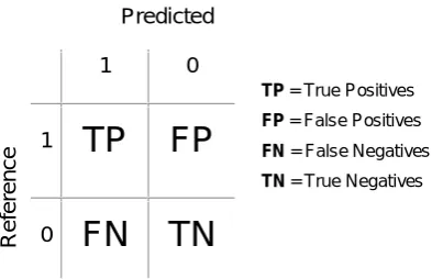
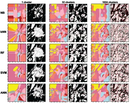
Figure 1.1 Schematic representation of data inference...2 Figure 1.2 Schematic representation of the process of deductive and inductive reasoning. ...3 Figure 2.1 An example of NB estimated joint (normal) class conditional probability densities for one discretised continuous variable and three classes. ...12 Figure 2.2 Schematic diagram of kNN classifications for a binary classification task in 2D variable space. Filled symbols represent predicted class for an unlabelled sample. ...14 Figure 2.3 Schematic representation of binary DT classifier architecture. Split nodes partitions inputs based on some threshold (for continuous data)...17 Figure 2.4 SVM schematic diagrams of a) separating hyperplane in 2D variable space, where indicates class a and class b. Filled symbols represent support vectors. b) Kernel transformation example from 1D variable space to 2D kernel space...21 Figure 2.5 Schematic diagram of a) single McCulloch–Pitts neuron. ...24 Figure 2.6 Generalised workflow for machine learning supervised classification. ...25 Figure 2.7 Confusion (error) matrix for binary classifications showing the relationships between True and False, Positives and Negatives. ...30 Figure 2.8 Schematic diagram representing the effect of noise and the bias2-variance decomposition and its relationship to classifier complexity (under-fitted and over-fitted models) and error...31 Figure 2.9 Example of k-means (k = 3) clustering in 2D variable space. Filled symbols represent cluster centroids and lines indicate boundaries between clusters. ...34 Figure 2.10 Example of a dendrogram with five clusters as output from hierarchical clustering, similar clusters reside on the same branch of the dendrogram. ...35 Figure 2.11 Schematic diagram of SOM unsupervised clustering algorithm structure, after Bierlein et al. (2008). ...37 Figure 4.1 Reference geological map, after Buckley et al. (2002) and associated class proportions for the 13 lithological classes present within the Broken Hill study area. ...75 Figure 4.2 Example of Taspatial distributions for 1, 32 and 1024 clusters ...77

Figure 4.3 Mean ranked normalised variable importance for 1, 32 and 1024 Ôaclusters using all data after the

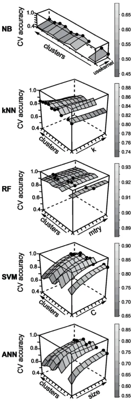
removal of highly correlated variables. ...80 Figure 4.4 Comparison of MLA cross-validation accuracies as a function of classification model parameter and number of Taclusters ...81

Figure 4.5 Comparison of MLA mean Tbaccuracy with respect to variations in the number of Taclusters ...82

Figure 4.8 Visualisation of the spatial distribution of MLA lithology class predictions using spatial coordinates and geophysical data (All Data) as inputs ... 87 Figure 4.9 Comparison of MLA training (using 10-fold cross-validation) and prediction processing times.. 88 Figure 5.1 Schematic diagram of RF decision tree architecture... 99 Figure 5.2 Idealised SVM decision boundary for a 2D (ܠ1andܠ2) non-separable linear binary classification problem...100 Figure 5.3 Mapped lithologies, after Buckley et al. (2002) within the Broken Hill sample area, western New South Wales, Australia. ...102 Figure 5.4 Comparison of the spatial distribution of uncertainty estimated from the class membership probabilities generated by RF and SVM using 0.02, 0.05 and 0.10 Tasample proportions. ...107

Figure 5.5 Tberror-uncertainty thresholds for 0.05 Tasample proportion ...108

Figure 5.6 Comparison of RF and SVM Tbaccuracy (100 groups of 1000 samples) as a function of Tasample

size compared with Tbaccuracies generated after uncertainty thresholds applied (see Table 5.2) ...110

Figure 5.7 Difference between RF and SVM recall and precision rates for the 13 classes in the Broken Hill study area. ...112 Figure 5.8 Comparison of the spatial distribution of RF and SVM lithology predictions and unclassified samples identified using uncertainty thresholds using 0.05 Tasample proportions. ...113

Figure 6.1 Map of Tasmania. Black rectangular region indicates the location of the Hellyer–Mt Charter region...122 Figure 6.2 Typical regional tectonic and geological setting of bimodal-felsic VHMS ore deposits...124 Figure 6.3 Diagram of VHMS a) footwall and b) hangingwall hydrothermal alteration zones in the Hellyer– Mt Charter region ...125 Figure 6.4 Interpreted geological map of Hellyer–Mt. Charter region, after Richardson (1994). ...127 Figure 6.5 Examples of pre-processed (non-standardised) soil geochemical, airborne geophysical and Landsat ETM+ data used in this study...132 Figure 6.6 a) Location of the 2100 Tasamples used to optimise RF classification model parameters, select

relevant variables and train RF classification models and b) individual class proportions of the total number of samples within the Hellyer–Mt Charter region...133 Figure 6.7 a) RF variable selection cross-validation accuracy. b) Final list of selected variables in ranked order of relative importance based on mean decrease in RF Gini Index...134 Figure 6.8 Comparison of: a) interpreted geological map; b) lithology predictions; c) spatial distribution of inconsistencies between the pre-existing interpreted geological map and RF predictions; and d) spatial distribution of RF prediction uncertainty...139 Figure 6.9 Results of SOM unsupervised clustering for the Hellyer Basalt divided into four sub-classes ....142 Figure 6.10 SOM sub-classes identified in a) Lower Basalt, b) feldspar-phyric andesite and c) hangingwall andesite units of the QHV. The y-axes of variable frequency plots represent frequency densities. ...143 Figure 7.1 Study region location and generalised lithologic units, modified from Mineral Resources Tasmania (2011). Table 7.1 provides a summary of class descriptions and abbreviations. ...156 Figure 7.2 a) Example of Ta samples locations. Note Qs class was not included in Ta. b) Class proportions

samples of Qs class not included in Tbfor classifier evaluation. Table 7.1 provides a summary of class

descriptions and abbreviations. ...161 Figure 7.3 Segmented images derived using 100 SOM nodes for a) standard variables and b) texture variables. Note the colour ramp is repeated resulting in duplicated segment colours...163 Figure 7.4 Comparisons of spatial-contextual classifier Tb accuracies. ...167 Figure 7.5 Selection of the best performing spatial-contextual RF classifiers. Table 7.1 provides a summary of class descriptions and abbreviations...168 Figure 7.6 Example of best performing spatial-contextual SVM classifiers. Table 7.1 provides a summary of class descriptions and abbreviations...169 Figure 7.7 Example of RF and SVM classifications trained on standard variables...171 Figure 7.8 Comparisons of mean proportions (across 10 Ta and Tb resamples) of mapped Qs samples

classified as classes present within Ta...172

Figure 8.1 RF partial dependence plots showing the relative influence of variables on the prediction presence of QHV units...196 Figure A.1 Image (input variable) used for MLA supervised classification training and testing. Random values between 0 and 1 are assigned using a uniform distribution. ...255 Figure A.2 Three class example of Tarandom sampling (points) and Tb(background) sample structure for

trials 1–4. ...256 Figure A.3 MLA prediction accuracy distribution boxplots for six classes given “no-information” with four combinations of Taand Tbclass distributions (Table A.2)...257

Figure A.4 Trial 2 MLA normalised Tbaccuracy density distributions and associated p-values (black lines)

for c = 6. Ta class proportions are equal, i.e. 0.1667, Tb class proportions are equivalent to those

L

IST OF

A

BBREVIATIONS

0D - no temporal or spatial (data) dimensions 1D - one temporal or spatial (data) dimension 2D - two spatial (data) dimensions

3D - three spatial (data) dimensions AEM - Airborne Electro-Magnetics ANN - Artificial Neural Networks

ASTER - Advanced Spaceborne Thermal Emission and Reflection Radiometer AVIRIS - Airborne Visible/Infra-Red Imaging Spectrometer

BHD - Broken Hill Domain

BN - Bayesian Networks

BT - Boosted Trees

BvSB - Best-versus-Second-Best

CSIRO - Commonwealth Scientific and Industrial Research Organisation DEM - Digital Elevation Model

DT - Decision Trees

ETM - Enhanced Thematic Mapper GIS - Geographic Information System GLCM - Grey Level Co-occurrence Matrices GPR - Ground Penetrating Radar

GRS - Gamma-Ray Spectrometry

ICT - Internet Communication Technology

IEEE - Institute of Electrical and Electronics Engineers kNN - k-Nearest Neighbours

LDA - Linear Discriminant Analysis LiDAR - Light Detection and Ranging MCMC - Markov-chain Monte Carlo MLA - machine learning algorithm MLC - Maximum Likelihood Classifier MLP - Multi-Layer Perceptrons

NeCTAR - National eResearch Collaboration Tools and Resources

NIR - Near Infra-Red

PCA - Principal Component Analysis PKPD - Price, Knerr, Personnaz & Dreyfus PNN - Probabilistic Neural Networks PR - post-regularisation

QDA - Quadratic Discriminant Analysis QHV - Que–Hellyer Volcanics

RBF - (Gaussian) Radial Basis Function

RF - Random Forests

RTP - Reduced-To-Pole

SAM - Spectral Angle Mapper SAR - Single-Aperture Radar SLP - Single-Layer Perceptrons SOM - Self-Organising Maps

SPOT - Satellite Pour l'Observation de la Terre SVM - Support Vector Machines

SWIR - Short Wave Infra-Red

T - labelled samples available for supervised classification

Ta - portion ofTused for classifier training and validation (training data)

Tb - portion ofTused for classifier evaluation (test data)

A

CKNOWLEDGEMENTS

This thesis would never have been completed, nor would my sanity have been preserved, without the calm and supportive mentorship of my supervisor Anya Reading. Anya, you taught me many things over the past four years, especially the courage to believe in myself. Special thanks must go to Andrew McNeill for being the secondary supervisor I never really had. Thanks also to Michael Roach for many frantic encounters in the corridor. Sorry I forgot to acknowledge you in my Honours thesis. I hope this makes up for it. Thanks to Daniel Bombardieri, Jocelyn McPhie, Ron Berry and Jacqueline Halpin for providing comments on my work. Thanks also to the other staff and students, especially Selina Wu, Jeff Steadman and the quiet but resourceful “geofizz” nerds on the top floor (you know who you are), at the ARC Centre of Excellence in Ore Deposits (CODES) and the School of Earth Sciences, University of Tasmania.

Over the past three years I have had the pleasure of visiting and networking with researchers based at other universities across Australia. Thanks to: Malcolm Sambridge, Simone Pilala and Thomas Bodin at the Research School of Earth Sciences, Australian National University; Steve Micklethwaite, Mark Lindsay and Eun-Jung Holden at the Centre for Exploration Targeting, University of Western Australia; and Thomas Landgrebe, Simon Williams and Dietmar Müller from the EarthByte Group, University of Sydney. Meeting you all and discussing different aspects of my research, however briefly, has enriched my Candidature.

I must acknowledge the universe for star dust, gravity and the internet (does that mean I have to thank Telstra?!). I wouldn’t be here without you. Also, thanks to those I haven’t thanked, especially my caving buddies at STC. I will go caving again one day!

C

HAPTER

1 – I

NTRODUCTION

Recent and rapid technological advances in geoscience data capture and storage are significantly increasing the volume and variety of data available to geoscientists (Kraut & Wettergreen 2010; Bhatia et al. 2013; Sellars et al. 2013). Vast amounts of continuously collected data, coupled with large volumes of pre-existing data, presents challenges to large scale manual and/or deterministic analysis and interpretation within acceptable time frames (Feyyad 1996; Miller & Han 2001; Kraut & Wettergreen 2010). This is because humans, despite being good at pattern recognition, are limited in the amount of data they can process and analyse at any given time. Furthermore, as models of natural phenomena grow in complexity, i.e. number and variety of inputs (variables) and outputs (target phenomena) increases, understanding the causal relationships amongst model elements becomes increasingly difficult (Reitsma 2010). As a result, we are likely to be missing opportunities to gain knowledge from interactions between multiple layers of disparate data, thus limiting our understanding of complex Earth systems (Feyyad 1996).

Human senses receive information, the source of which is then immediately and subconsciously identified (Ripley 1996). Take for example, the observational and cognitive skills that geologists employ to recognise and assign physical Earth objects and features to predefined categories. The category or class to which an object or feature belongs is determined by a set of consistent rules geologists acquire and learn during years of training. The categorisation of geological features forms the basic premise geologists use to map or model geological phenomena. Geological maps are the fundamental sources of information that geologists use to interpret and understand complex Earth systems.

1.1. Machine learning

The science of learning from data is a key focus of machine learning. Machine learning combines the fields of statistics and computer science for pattern recognition and data mining applications (Michie et al. 1994b; Ripley 1996; Hastie et al. 2009). For science based research, pattern recognition is the process of discovering, via automated or semi-automated statistical methods, useful patterns within data (Kotsiantis 2007). Discovered patterns are then used to generate predictions based on similar data (Ripley 1996). The essence of machine-assisted pattern recognition is to provide computers with the ability to adapt their decision structures, based on the characteristics of observed data and generate valid and objective predictions (Schölkopf 2003). Machine learning is an extension of the pattern recognition process. It attempts to provide users with an understanding of the patterns within data (Feyyad 1996; Witten & Frank 2005). Hence, machine learning outputs should be comprehensible in a way that allows interpretations to be formulated in response to the decision structures used to recognise and exploit patterns within data and generate predictions (Feng & Michie 1994; Henery 1994a; Ripley 1996).

Data inference is the act of gaining information, knowledge and ultimately wisdom, from the analysis of raw data using statistical methods (Fotheringhamet al.2002; Mucke 2009). The process of data inference can be divided into three levels of understanding (Figure 1.1). The foundation for these levels of understanding is raw data. Successive levels of data inference distil and refine raw data until a complete understanding of the mechanisms controlling the phenomena under investigation is realised (Mucke 2009). The conclusions attained via the process of data inference are subsequently applied to other similar data in

order to make predictions, formulate interpretations and inform the decision making process (Bousquetet al.2004).

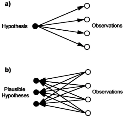
There are two logical approaches to data inference: deductive and inductive reasoning (Feng & Michie 1994; Sivia 1996; Gubbins 2004). Deductive approaches to inference usually involve a researcher (or analyst) who develops a hypothesis (or model) regarding some natural phenomenon. Observational data are then utilised to accept or reject the aforementioned hypothesis (Figure 1.2a). Deductive reasoning can be restrictive in its scope as the results of the analysis are constrained by the pre-formulated hypothesis. In contrast, inductive approaches to inference initially utilise available data/observations to identify patterns. Learned patterns are then employed to develop a range of plausible hypotheses (Figure 1.2b). The advantages of well-performing inductive approaches over deductive approaches to reasoning are based around the ability of computers to rapidly execute repetitive tasks on large digital datasets and infer plausible models without any preconceptions of their form or parameters (Sivia 1996; Burlet al.1998).

Machine learning algorithms (MLAs) are computational tools that provide analysts with a range of statistically sound methods for inductive data inference (MacKay 2003; Bousquet et al. 2004). MLAs inductively generate inferences from potentially high-dimensional

multivariate input data by constructing one or more plausible models that link observed data to the phenomena under investigation (Hastieet al.2009; Chipmanet al.2010). Both supervised and unsupervised approaches to machine learning are possible. During supervised learning, a model is induced from training data, or what is known about the problem, that best predicts samples contained within these data. Training is guided by the minimisation of some error or loss function based on the internal architecture of the learning algorithm (Bousquet et al. 2004; Hastie et al. 2009). In essence, supervised machine learning methods attempting to mimic human reasoning and learning and can be used either for classification or regression problems (Ripley 1996; Burlet al.1998; Witten & Frank 2005; Marsland 2009). In the unsupervised case, a learning algorithm is given unlimited scope in an attempt to find natural groups or clusters in data that best describe its inherent relationships (Ripley 1996; Hastieet al.2009).

1.2. Geological maps

A common task in the geosciences is the process of constructing a map1 from indirect observations that represents the location and/or properties of geological phenomena (Sambridgeet al.2006; Maiti & Tiwari 2010b). This task is traditionally approached using deductive reasoning in which forward modelling and/or inversion techniques are applied. The forward model represents what is known about the problem given a set of physical properties. Inversion then proceeds in an attempt to refine the proposed model to the observed data and the relevant physical properties of the target, i.e. the geological objects or features under investigation (Gubbins 2004).

Geological maps are essentially an abstracted representation of geologically significant features within a 2D spatial reference frame, typically lithological units. Geological maps are a fundamental base layer of information for a wide range of problems and applications (Thomas 2004) such as targeting ore deposits and hydrocarbon resources (Kusky & Ramadan 2002; Jackson 2005; Holden et al. 2008; Metelka et al. 2011; Shaheen et al. 2011), tectonic reconstructions (Dohm et al. 2007; Gibson et al. 2008; Leverington & Moon 2012), geohazard risk assessment and engineering applications (Tangestani 2004; Ramli et al. 2010; Stumpf & Kerle 2011; Sabatakakis et al. 2012), geomorphology and hydrology studies (Buselli & Lu 2001; Draskovits & Laszlo 2005) and ecological

1

modelling (Guisan & Zimmermann 2000; Anderson & Ferree 2010; Brown & Mies 2012). However, geological maps are commonly constructed from the subjective interpretations of a domain expert (the geologist) based on limited field observations. As a result, they are typically imprecise representations of the spatial distribution of geological materials (Bárdossy & Fodor 2001; Grebbyet al.2011; Lindsayet al.2013).

The collective experience and knowledge of a geologist is required to relate limited field observations and supplementary data such as geophysical measurements to geological phenomena. The expert subjective knowledge of a geologist, combined with often incomplete observations, the fact that geological and geophysical data contains some form of irreducible or deterministic noise (Scales & Snieder 1998; Ricchetti 2000; Link & Blundell 2003) and the nature of lithological units to exhibit a high degree of interclass similarities and intraclass variability (Ghimire et al.2010; Grebbyet al.2011), means that error and uncertainty are an ever present component of geological maps (Bárdossy & Fodor 2001; Gelfort 2006). Despite this, geological maps do not usually provide an indication of the uncertainty associated with its component elements. This is because it is difficult to quantify the confidence with which geologists have used to subjectively interpret the spatial distributions of lithologies during the construction of a geological map (Bárdossy & Fodor 2001; Lindsayet al.2013).

1.3. Research scope and hypothesis

Multivariate geospatial data, collected by airborne or spaceborne remote sensing platforms, complements the use of field observations for the construction of geological maps (Yanget al.1998; Shaheenet al.2011; Leverington & Moon 2012). Given the large quantity of this potentially useful data, MLAs have the potential to provide practical solutions for geological mapping applications in regions where collecting field observations is a costly, time consuming and challenging prospect. Furthermore, as MLAs require minimal user intervention in order to generate outputs, the subjectivity with which predictions are obtained is reduced (Henery 1994a; Ripley 1996). Therefore, MLAs offer an opportunity for geologists to semi-automate the process of creating first-pass geological maps of remote or inaccessible terrain using pre-existing multivariate geospatial data.

outcomes of research. This is because different learning strategies approach the task of supervised classification in contrasting ways. Given that Kotsiantis (2007) identifies five general machine learning strategies for supervised classification, different MLAs may be better suited to generating geological maps given the spatial context of geoscience data. Based on the motivations described above and the need to develop an understanding of the capabilities of different MLAs for geological mapping applications, my hypothesis is that it is possible to establish which MLAs are most suited to recurring geological mapping tasks using multivariate geospatial data. Suitability, in this context, is constrained by the requirement of MLAs to generate accurate and plausible map of the spatial distribution of geological features from the integration of disparate multivariate data, while also providing a means of gaining a high level of understanding of complex geological phenomena.

1.3.1. Major research questions to be addressed

I address the following major research questions:

1. What are the advantages and limitations associated with different MLAs in the context of geological mapping applications?

2. What are the best-practice approaches to integrating disparate geoscience data and implementing MLAs for practical real-world geospatial inference problems?

3. Is it possible to assign meaningful levels of confidence to the outputs of MLAs?

develop new functions or modify existing functions for specific purposes, which can be freely distributed to and adapted by other users.

1.4. Thesis structure

This thesis contains two review chapters followed by four chapters, formatted as manuscripts for publication, documenting groups of experiments conducted during the course of my research. The insights arising from the findings detailed in these chapters are synthesised and discussed in terms of their relevance to the hypothesis and research questions outlined previously. This is followed by a summary of key findings and conclusions.

A summary of the structure of this thesis and the contents of chapters are as follows:

Ø Chapter 2 provides a review of machine learning theory for supervised classification and unsupervised clustering algorithms and best-practice methods for their implementation.

Ø Chapter 3 reviews previous research using MLAs for geoscience classification applications. Specific focus is placed on the use of spatially distributed geoscience data for geological mapping.

Ø Chapter 4 – Cracknell & Reading (2014) published in Computers & Geosciences – documents a robust comparison of MLAs, each representing one of the five general machine learning strategies for supervised classification, applied to remote sensing geological mapping. In particular, this chapter focuses on the responses of machine learning strategies to the degree of spatial clustering represented by the training data and the inclusion of explicit spatial information.

Ø Chapter 5 – Cracknell & Reading (2013) published in Geophysics – addresses the estimation of meaningful measures of MLA prediction uncertainty as a mechanism for identifying ambiguous or erroneous classifications.

unsupervised (Self-Organising Maps) MLAs. This work demonstrates the use of machine learning for the critical assessment of pre-existing geological maps and for interpreting complex geological phenomena.

Ø Chapter 7 – to be submitted for publication in IEEE Transactions on Geoscience and Remote Sensing – investigates methods that provide MLAs with implicit spatial-contextual information for improving geological mapping outcomes.

Ø Chapter 8 presents a synthesis and discussion of the key findings in light of main research questions and aims. The significance of these findings, with respect to the implementation of MLAs for practical geoscience applications, is presented.

C

HAPTER

2 – M

ACHINE LEARNING THEORY AND

IMPLEMENTATION

This chapter documents a comprehensive review of machine learning algorithms (MLAs) for practical data inference problems. Initially, summaries of the motivations and best-practice approaches regarding the three fundamental stages that users must employ in order to implement MLAs for practical supervised classification applications are provided. This is followed by a review of the theory that underpins the five general MLA strategies for supervised learning. The advantages and limitations of these contrasting MLA strategies, as documented in published literature, are considered. This chapter concludes with a summary of MLAs for unsupervised learning and includes a description of the theory behind several well-known and popular clustering algorithms.

2.1. Machine learning

MLAs generate predictions by linking input data (variables) to desired outcomes (targets, Friedman 1997; Chipman et al. 2010). The nature of the inference problem is defined by the target data types provided to the MLAs during training. For example, the aim of classification is to generate predictions for a set of discrete classes that represent unordered descriptive categories. In contrast, the aim of regression is to predict ordered numeric values (Marsland 2009). This chapter does not address machine learning for regression problems as the objective of my research is to investigate MLAs for the classification of discrete categories representing geological features such as lithologies.

2.1.1. Supervised versus unsupervised learning

MLAs are employed to generate inferences from data (Friedman 1997) using either supervised or unsupervised approaches to learning. Supervised learning utilises training data and can be defined as function approximation (Kotsiantis 2007; Hastie et al. 2009) where the aim is to minimise an error or loss criterion (Kuncheva 2004; Marsland 2009). Training data comprises a set of discrete and unordered labels indicating known outcomes or observations. These data are used to induce or train a classification model that links variables to the classes present in the training data while minimising the error criterion. Once constructed, a supervised classification model enables one to predict the class labels of samples previously unseen by the MLA (Kuncheva 2004; Hastieet al.2009). In contrast to supervised approaches to learning, unsupervised learning only has a set of variables and no observed or prior knowledge of desired outcomes, i.e. it is data-driven (Ripley 1996). The lack of prior knowledge with which to assess the results of unsupervised learning means that the quantitative assessment of outputs is infeasible. Thus, the aim of unsupervised learning is not to minimise an empirical error function, it is to identify natural, coherent groups within data as a means of gaining insight into how these data are organised (Kuncheva 2004; Hastieet al.2009).

2.2. Supervised classification

Supervised classification can be formally described as linking one domain (input data) to another (target classes) via a discrimination function (without considering noise or random error):

Inputs (variables) are represented as dvectors of the form ۃܠ_ଵ,ܠ_ଶ, … ,ܠ_ௗۄand y is a finite set ofcclass labelsሼݕ_ଵ,ݕ_ଶ, … ,ݕ_௖ሽas indicated by the labelled data,T. Given instances ofܠ andݕ, supervised classification attempts to induce or train a classification model݂ᇱ, where ݂ᇱ _{݂such that,}

ݕො=݂ሺܠሻ, [2.2]

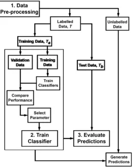
which links variables to classes (Gahegan 2000; Hastieet al.2009; Kovacevicet al.2009). The form of ݂ᇱis induced by some internal strategy that minimises the empirical error (Kohavi 1995; Schölkopf 2003; Hastie et al. 2009). In other words, given the architecture of a particular MLA, decision structures are induced that reduce the cost of classification, i.e. misclassifications, to a minimum given the information within T. In practice, as we only have class labels for a limited set of data, it is necessary to divide available data into independent groups for MLA training, Ôa (training data) and evaluation, Ôb (test data,

Witten & Frank 2005; Hastieet al.2009).

2.2.1. Classification strategies

This section outlines fundamental theory behind the five general machine learning strategies for supervised classification (Kotsiantis 2007): statistical learning algorithms; instance-based learners; logic-based learners; Support Vector Machines; and Perceptrons.

2.2.1.1. Statistical learning algorithms

Statistical learning algorithms construct an explicit statistical model that estimates the probability that a sample belongs to a particular class (Domingos & Pazzani 1997; Guyon 2009). These include, Linear (and Quadratic) Discriminant Analysis (LDA, QDA) which use density estimation techniques to find linear (or quadratic) combinations of variables that best separate multiple classes (Kotsiantis 2007). Alternatively, Bayesian models such as Naïve Bayes (NB) and Bayesian Networks (BN) provide methods for probabilistic supervised classification. These methods are superior to LDA or QDA for problems represented by high-dimensional inputs variables that exhibit non-linear relationships between multiclass targets (Witten & Frank 2005).

Theorem, which states that the probability, P, that a class ݕis correct given the data ܠ using,

Pሺݕȁܠሻ= ୔ሺܠȁ௬ሻ_୔(×_ܠ)୔(௬). [2.3]

Pሺݕሻis the prior probability and represents our knowledge of the problem, i.e. Ta.Pሺܠȁݕሻ

is the probability that the data is true given the class and represents the likelihood function used to update the prior via empirical analysis. P(ܠ) indicates the data used during analysis, which is constant for all classes, thus it can be ignored for most applications (John & Langley 1995; Sivia 1996; Domingos & Pazzani 1997). To simplify the problem, NB assumes that for a given class the input variables are independent of each other. This assumption yields a discrimination function indicated by the products of the joint probabilities that the classes are true given the data for samplei, represented by a vector of inputsܠwith valuesݑ_௜:

݂ (ܠ௜) =P(ݕො)ς௩ௗୀଵP(ܠ=ݑ௜|ݕො). [2.4]

Using this logic, the problem can be reduced to finding a vector of probabilities where the Bayes optimal classifier is represented by the maximal class probability (Figure 2.1, Duda & Hart 1973; Molinaet al.1994; Hastieet al.2009).

NB is not prone to overfitting (see Section 2.2.2.3, Guyon 2009) and often outperforms more sophisticated alternatives unless ܠcontains correlated and hence non-independent

variables (Domingos & Pazzani 1997; Witten & Frank 2005; Tanet al.2006; Hastieet al. 2009). Non-independent variables skew the NB learning process such that discrimination will effectively be concentrated on the set of dependent variables (Witten & Frank 2005). Furthermore, NB is limited where a given variable does not occur in conjunction with every class in Ta. In this case, the probability of a variable leading to the class in question

would be zero. As the final probabilities for a given class are the product of all the probabilities, the resultant will also be zero (Witten & Frank 2005; Kotsiantis 2007). The default NB formulation assumes normally distributed continuous variables. In cases where this assumption does not hold, kernel density estimation procedures that do not assume a particular distribution will improve performance (John & Langley 1995; Witten & Frank 2005).

BN (or Directed Acyclic Graphs, Pearl 1988; Ripley 1996) are an extension of NB that does not assume independent variables (Witten & Frank 2005). BN construct a graphical (network) model where nodes represent a variable and the links between nodes represent the correlation between variables. The local conditional probability distributions of a variable given its parents are represented by a set of tables, one for every linked variable. From these tables, joint probability distributions are calculated based on the independence structure within the network (Friedman et al. 1997). In circumventing the assumption of independence, calculating posterior probabilities using all data becomes computationally expensive or infeasible for large numbers of variables (Kotsiantis 2007).

An alternative approach to inducing BN is to approximate posterior probabilities using Markov-Chain Monte Carlo (MCMC) methods. MCMC, in the context of BN, is used to randomly sample variables and then weight these samples by their likelihood functions. As the number of samples increases the closer the estimation converges on their expected values (Marsland 2009). Further reductions in processing time can be obtained by only assessing a variable, its child nodes and the parent nodes of those child nodes, termed a Markov blanket. The nodes within a Markov blanket are conditionally independent of all other nodes, therefore, the variable they represent is irrelevant and not required to estimate the likelihood function (Witten & Frank 2005; Marsland 2009).

significant difference between the predictions generated by NB or those of BN (Dumaiset al.1998). Experiments conducted by Friedmanet al.(1997) showed that in many cases NB generated significantly more accurate predictions than BN.

2.2.1.2. Instance-based learners

Instance-based learning algorithms, also known as lazy learners, feature three unique characteristics that distinguish them from other learning strategies: (1) Ta is stored until

required to generate predictions for individual samples; (2) predictions are formulated by combining samples in Ta; and (3) they discard predictions once they have been generated

(Aha 1997; Wettscherecket al.1997). Unlike many other MLAs, which construct a global classification model based on all the samples in T_a, instance-based learners train a single classifier for every sample requiring prediction. The most commonly used instance-based learning algorithm isk-Nearest Neighbours (kNN, Atkesonet al.1997).

For an individual sample that requires classification, the kNN algorithm queries a selected representative, i.e. the closest neighbours, ofT_athat reside within a local region of variable space (Bottou & Vapnik 1992; Atkeson et al. 1997). This algorithm, developed by Fix & Hodges (1951) and Cover & Hart (1967) is based on the assumption that the sample to be classified is most likely to be proximal to the most abundant class contained within neighbouring observations in d-dimensional variable space (Henery 1994a; Wettschereck et al. 1997; Witten & Frank 2005; Tan et al. 2006). Thus, the majority class within neighbouringTa samples defines the predicted class label (Figure 2.2). In situations where

multiple maximal classes are identified within a local neighbourhood one of these classes

is randomly selected (Kotsiantis 2007).

The kNN algorithm can be defined formally as:

ݕො= max௖൫σ ܫ௞௝ୀଵ(ݕ௝= ܿ)൯, [2.5]

whereܫ(ݕ_௝= ܿ) is an indicator function that identifies thekneighbouringTasamples equal

to class c. It is important to select an appropriate value of k, the number of nearest neighbours to assess. Too small a value of k often results in underfitting (see Section 2.2.2.3) and susceptibility to noise. Conversely, too large a value of k will generate classifiers that are over-fitted and more likely to misclassify a Tb sample due to the

presence of samples belonging to another class. Typically, methods such as cross-validation are required to select appropriate values ofk(Tan et al. 2006; Kotsiantis 2007; Hastieet al. 2009).

In conjunction with the selection of an appropriate value of k, a similarity or distance measure is used to establish the k closest neighbours in variable space. The most commonly used similarity measure is the Euclidian distance metric, although other metrics that measure proximity between samples in variable space are possible. These metrics include the Manhattan and Minkowsky distances (Table 2.1, Hechenbichler & Schliep 2004; Kotsiantis 2007). As the proximity of T_a samples is established using relative distances in variable space scaling can be an issue. Therefore, it is recommended that continuous variables be standardised to a common scale, especially if the variables used as input are measured in different units (Molina et al. 1994; Kotsiantis 2007; Hastie et al.

Euclidian ܦሺݔ,ݕሻ=ඩ෍ ȁݔ௜ ݕ௜ȁ ௡

௜ୀଵ

Manhattan ܦሺݔ,ݕሻ=෍ ȁݔ௜ ݕ௜ȁଶ ௡

௜ୀଵ

Minkowsky ܦሺݔ,ݕሻ=ඩ෍ ȁݔ௜ ݕ௜ȁ௥ ௡

௜ୀଵ

ೝ

2009). In addition, it is easier to implement kNN using numeric variables as the distance between values is explicit rather than with categorical variables where some notion of similarity, i.e. normalisation, is required to provide a measure of scale (Witten & Frank 2005).

As all variables are treated equally by kNN, it is affected by redundant, irrelevant or noisy variables (Henery 1994a; Wettschereck et al. 1997; Hechenbichler & Schliep 2004). In addition, the computational cost of finding neighbours and storing Tacan be excessive for

large numbers of samples (Molina et al. 1994; Hastie et al. 2009). Despite this, kNN has been shown to perform well in situations where decision structures, i.e. the separation of classes in variable space, are highly irregular (Hastie et al. 2009). Furthermore, unlike logic-based learners or Perceptrons, kNN will usually generate stable predictions in light of changes inTa(Breiman 1996).

The standard kNN algorithm assumes that the k neighbouring T_a samples to the sample requiring prediction are of equal importance. Equal weighting ofk proximal samples can incorporate redundant, irrelevant or noisy variables in the resulting classification model resulting in poor performance (Wettschereck et al. 1997). Moreover, the standard kNN algorithm is vulnerable to high bias (see Section 2.2.2.3) when faced with high-dimensional inputs (Friedman 1994; Hastie & Tibshirani 1996). Adjusting training sample weights using monotonically decreasing distance decay functions emphasises the contribution of proximal neighbours on predictions, thus dampening the potential for over or underfitting (Hechenbichler & Schliep 2004). Sample weighted kNN proceeds using a weighted majority vote:

ݕො= max௖൫σ ݓ௞௝ୀଵ ௝ܫ(ݕ௝= ܿ)൯, [2.6]

whereݓ_௝indicates a weighting function based on the distance metric selected.

Adaptive kNN algorithms utilise methods that identify different values of k for a given class and/or sample. Alternatively, they modify the geometry of the search neighbourhood based on input variability (Hastie et al. 2009). Dietterich & Wettschereck (1994) outline several approaches to computing optimal local values of k. The standard local adaptive kNN (called kNNunrestricted), on which all other variants are based, uses cross-validation to

identify k values that correctly predict individual Ta samples. To classify a given sample,

majority of these samples are selected. Friedman (1994) describes the Flexible Metric Nearest Neighbour algorithm, an adaptive form of kNN that adjusts the geometry of the search region based on the local relevance of variables via recursive partitioning. An optimal k value is selected by iteratively adjusting distance metrics orthogonal to variable space axes. This generates elongate search neighbourhoods in directions where there is very little observed variability in class probabilities (Molina et al. 1994; Hastie et al. 2009). Using a similar approach, Hastie & Tibshirani (1996) developed a Discriminant Adaptive-nearest Neighbour algorithm that incorporates local LDA to estimate optimal distance metrics for adjusting search neighbourhoods parallel to the axes of variable space.

2.2.1.3. Logic-based learners

Logic-based learners use a set of criteria or rules in order to generate predictions. The simplest forms of logic-based learners incorporate a series of Boolean decisions (“and”, “or”, “if else”) that, in the context of machine learning, are automatically generated and define classification rules (Feng & Michie 1994; Witten & Frank 2005). Logic-based classification models map classes to variables by dividingTainto discrete partitions of

self-similarity (Henery 1994a). These partitions must classify a minimum number of Ta

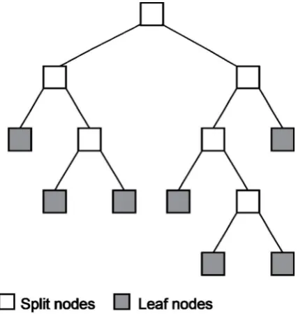
samples belonging to the classes split under the current rule (Feng & Michie 1994). Decision Trees (DT) provide a concise representation of logic-based learners (Witten &

Frank 2005) and are the foundation for more sophisticated algorithms that use this learning strategy. Breiman et al. (1984) pioneered the widespread use and implementation of DT under the pretence that they generated accurate predictions while also providing a basis for understanding the structural relationships between target classes and input variables.

DT apply conditions to a particular variable and then splits Ta based on thresholds or

Boolean decision rules (Feng & Michie 1994; Witten & Frank 2005). DT comprise a series of nodes in a cascading top-down inductive network. From each “parent” node data is split into “child” nodes that are either branching nodes, where data is subjected to splitting again; or leaf nodes, where the resulting class is put forward as a prediction (Figure 2.3). DT are constructed from a root node, the initial starting node of the trees and grown recursively unlit some stopping criterion is reached, such as the minimum purity of the leaf nodes (Breimanet al.1984). Numeric inputs are dealt with by spitting on threshold values, i.e. using greater than or less than rules, at an established point within the numeric range of a given variable (Witten & Frank 2005).

A special form of DT are the Classification and Regression Trees (CART) developed by Breiman et al. (1984). CART are binary DT that split parent nodes into two child nodes, thus avoiding the rapid fragmentation of data as can occur with multi-way spits (Hastie et al. 2009). CART use the information gain ratio (Gini Index) to defined an optimum splitting threshold for branching nodes (Breiman et al. 1984). The Gini Index calculates the information purity of child nodes with respect to that of their parent node by comparing the ratio of classes passed onto a child node. The Gini Index is defined as:

ܩ݅݊݅(ݐ) =σ ݃௝௖ୀଵ ௖ሺ1 ݃௖ሻ, [2.7]

where݃_௖is the probability or the relative frequency of classcat nodejand is given by:

݃௖= ௡_௡೎, [2.8]

possible benefit (information) for splitting a node with only one class (Witten & Frank 2005).

CART employ a tree pruning method that strives to generate small trees while maintaining accurate estimates of the true probabilities of misclassification. Small trees are advantageous as they are often easier to interpret, reduce computational cost and are less prone to overfitting (Kotsiantis 2007). Pruning trees by replacing a sub-tree (series of nodes linked to a common parent node) is designed to address the trade-off between simplicity and accuracy (Feng & Michie 1994; Witten & Frank 2005).

DT are challenged by the presence of missing values (Witten & Frank 2005) and sensitive to small changes inTa. In these situations, DT can generate significantly different splitting

thresholds, which result in high variance (see Section 2.2.2.3). Ensemble methods, or a committee of classifiers, minimise the instability of DT by combining the results of multiple classifiers (Kuncheva 2004; Hastie et al. 2009). There are two basic algorithms that use multiple DT to cast a vote on the predicted class: Random Forests™ (RF), trademark of Leo Breiman and Adele Cutler; and Boosted Trees (BT, Banfieldet al.2007; Guyon 2009; Waske & Braun 2009).

RF, developed by Breiman (2001), is an ensemble classification scheme that utilises a majority vote for class association based on the results of multiple randomised DT, known as a forest. Randomness is introduced into the algorithm by randomly subsetting a predefined number of input variables (mtry) to split at each node of individual DT and by bagging (bootstrap aggregation). Bagging (Breiman 1996) generates Ta samples for each

tree by sampling with replacement a number of samples equal to the number of instances inTa. This equates to approximately two-thirds of samples available for training while the

remaining samples are used for evaluation. Bagging is reported to improve classification predictions as long as they are not stable in the presence of alteredTa(Breiman 1996). The

Gini Index is used by RF to determine a “best-split” threshold at each node of individual DT. RF grows multiple DT and is generally insensitive to noise and model overfitting (Breiman 2001; Tanet al.2006).

samples that are difficult to classify by assigning higher weights to samples misclassified in the previous iteration, thus forcing BT to concentrate on correctly classifying these samples. The final result is obtained by combining all iterations (trained DT) using a weighted majority vote that emphasises the influence of more accurate DT in the ensemble (Freund & Schapire 1996; Banfieldet al.2007; Hastieet al.2009).

2.2.1.4. Support Vector Machines

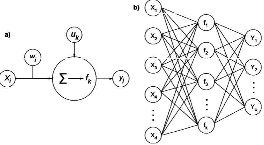
Support Vector Machines (SVM) are popular MLAs first described by Vapnik (1995; 1998). They have the ability to define decision boundaries between classes in a high-dimensional variable space by maximising the margin between two classes (Karatzoglouet al.2006; Hsuet al.2010). This approach to separating classes has been shown to reduce an upper bound on prediction error (Kotsiantis 2007). Furthermore, SVM training will always find a global minimum in contrast to other algorithms such as Artificial Neural Networks (Burges 1998; Kotsiantis 2007).

Basic SVM theory states that for a linearly separable dataset containing points from two classes there are an infinite number of hyperplanes that divide these classes. The hyperplane,h, is formally defined by:

࢝ ܠ+ܾ= 0, [2.9]

where࢝andbare solved via quadratic optimisation. The separation of two classes viahis achieved using only a subset ofTa instances known as support vectors (Tan et al. 2006).

SVM model complexity is unaffected by the number of variables because the number of support vectors identified is usually small. Thus, SVM circumvents the “curse-of-dimensionality” (see Section 2.2.3.1), i.e. the proliferation of variables causing intractable complexity and overfitting (Burges 1998). For this reason, SVM are well suited to deal with learning tasks where the number of variables is large with respect to the number of samples inTa(Kotsiantis 2007).

The maximum margin M (distance), equal to ૛

ԡ௪ԡperpendicular to h that separates the classes in question is taken to represent the optimal decision boundary. Obtaining M is equivalent to minimising the objective function:

݉݅݊࢝,௕ԡ࢝ԡ

మ

ଶ, [2.10]

Classifications are obtained by assessing which side ofhthe sample requiring a class label resides (Burges 1998).

In non-separable linear cases, SVM find h while incorporating a cost parameter C, which adjusts the penalty associated with misclassifying support vectors (Figure 2.4a). High values of C generate more complex prediction functions in order to misclassify as few support vectors as possible by way of a high penalty on error (Burges 1998; Karatzoglouet al. 2006). The objective function must be modified to incorporate this penalty term for wide margined decision boundaries with misclassifiedTa:

݉݅݊࢝,௕,కԡ࢝ԡ

మ

ଶ +ܥσ ߦே௜ୀଵ ௜, [2.11]

subjecttoݕ௜ሺ࢝.ܠ࢏+ܾሻ 1 ߦ௜,݅= 1,2, … ,ܿ,

where slack variables ߦ_௜ 0 represent the distance to misclassified support vectors from their respective marginal hyperplanes (Hsuet al.2010).

For non-linear cases, SVM use an implicit transformation of input variables via a kernel functionkern:

݇݁ݎ݊(ܠ௜,ܠ௝)=ۃ૖ሺܠ௜ሻ,૖൫ܠ௝൯ۄ, [2.12]

which returns the inner product between the positions of pairwise compared input variables (ܠ_௜andܠ_௝) in variable space (Figure 2.4b). The kernel function allows SVM to handle

linear relationships efficiently between classes and variables by projecting samples from the original d-dimensional variable space into a potentially infinite dimensional kernel space (Burges 1998; Hsu et al. 2010). It is important to select an appropriate kernel function from which T_a will be classified (Burges 1998; Kotsiantis 2007). Linear and Gaussian Radial Basis Function (RBF) kernels (Table 2.2) offer good first-choice kernels for most applications (Karatzoglouet al.2006).

The architecture of SVM described above deals with binary classification tasks. SVM can be extended to multiclass problems by combining multiple classifiers (Kotsiantis 2007). Two methods for combining SVM classifiers appear in the literature, both of which are based on a majority vote. The one-against-all method trains a number of classifiers equal to the number of classes inTa, with each classifier separating one class from the rest (Burges

1998). In contrast, the one-against-one method constructs ௖ሺ௖ିଵሻ

ଶ pairwise classification models, separating one class against another. Despite constructing more classifiers, the one-against-one method has been shown to efficiently generate robust classifications (Hsu & Lin 2002; Karatzoglouet al.2006; Kovacevicet al.2010).

Unlike other machine learning strategies, SVM do not employ density estimation to discriminate classes. In contrast, SVM exploit the geometrical characteristics of data by assessing only support vectors in order to geometrically define decision boundaries (Burges 1998; Melgani & Bruzzone 2004). However, SVM performance is sensitive to the choice of kernel, the size of the kernel, ó, used construct the transformed variable space andC(Hsu et al.2010). Therefore, Hsuet al.(2010) suggest using k-fold cross-validation to assist in establishing optimal SVM parameters for the intended application. In addition, it is recommended that input variables be standardised to a common scale (Hsu et al. 2010).

Linear ݇݁ݎ݊ሺܠ,ܠሻ=ሺܠ,ܠሻ

RBF ݇݁ݎ݊ሺܠ,ܠሻ= exp( ߪหܠ,ܠห૛)