Cauchy-Characteristic Extraction and Tidal Splicing
Thesis by
Kevin Barkett
In Partial Fulfillment of the Requirements for the Degree of
Doctor of Philosophy
CALIFORNIA INSTITUTE OF TECHNOLOGY Pasadena, California
2019
c 2019 Kevin Barkett
ORCID: 0000-0001-8230-4363
ACKNOWLEDGEMENTS
An undertaking of this size is not possible without the support and assistance provided by the many wonderful and fantastic people in my life:
To my loving parents, for having my back through all of these long years since I was a wee little lad. After nearly years, I’m finally getting out of school and moving into the real world!
To Mark Scheel and Yanbei Chen for advising me over these many years, putting up with the slow plod through these projects, and for all of the useful tools and skills I have learned.
To Jonathan, Vijay, Masha, and Matt G., and all of the other NR peers I’ve chatted with, for all of the nerdy, science discussions
To the Friday Night Dinner group, for the years of constant fun and turmoil as we horribly botched our way through a couple of campaigns
To Carla Corbit and Margo Miller, for all of the great times I have had working together with you during the practices, and especially during the fencing tournaments.
To all the crazy kids on the Caltech fencing team, for making practices and tournaments such fun to be a part of.
To JoAnn Boyd, for all the goofy faces, terrible (amazing) puns, and timely procrasti-chats.
To Sherwood, Jonas, Mike, Matt O., Denise, and all of the other cool cats on 3rd floor Cahill, for all of the fun moments between working hours.
To Sarah Gossan, for always bringing glam, glitter and cheer to the office, as well as a touch of that quintessentially British flair.
To John, Yeou, Mary, Steven, Andrew, Cameron, and all my buddies from before Caltech who have put up with my weirdness longer than most.
To Nicole Crione and all of the wonderful people I’ve met at her creative writing workshops over the past couple years.
To all of my other peers, collaborators, friends and relatives who’ve helped me on my journey.
ABSTRACT
As the aLIGO and Virgo detectors continue to improve their sensitivity for observing gravitational waves from merging compact binaries, they will require ever more precise theoretical predictions to extract a detailed understanding of the physics governing these merging systems. This thesis dis-cusses advancements within computing the gravitational waveforms along two avenues of research: the continued development of a spectral Cauchy-Characteristic Extraction (CCE) code and the pre-sentation of a novel method called ‘Tidal Splicing’ for generating waveforms for binary neutron star (BNS), black hole-neutron star (BHNS), and even Beyond GR systems.
Due to the finite extents of typical 3+1 simulations of merging binaries, the waveforms they gener-ate can suffer from near-zone effects and lingering gauge ambiguities. CCE was developed in order evolve radiating gravitational waves as they propagate outward to future null infinity, allowing stud-ies connecting the dynamical spacetime of binary evolutions to effects seen by distant observers, such as superkicks, and angluar and linear momentum fluxes. A recent spectral version of CCE showed promising improvements in accuracy and efficiency over the older finite-differencing code, PittNull. However, lingering issues with the numerics and implementation of the theory prevented it from wide spread use. We detail the developments updated its initial release and demonstrate the enhancement in accuracy they yield beyond the capabilities of PittNull.
PUBLISHED CONTENT AND CONTRIBUTIONS
Barkett, K. and Scheel, M. A. and Szilágyi B. (2019). “Spectral Cauchy-Characteristic Extraction of gravitational wave news”. In Preparation.
K.B. participated in the conception of the project, improving the numerical methods, perform-ing the tests of the code, and writperform-ing the manuscript
Barkett, K. and Scheel, M. A., et al. (2016). “Gravitational waveforms for neutron star bina-ries from binary black hole simulations”. In: Phys. Rev. D. 93(4):044064, Feb 2016. doi:
10.1103/PhysRevD.93.044064)
K.B. participated in the conception of the project, deriving the underlying theory, performing the comparisons and analysis, and writing the manuscript.
Barkett, K. and Chen Y. and Scheel, M. A. and Varma V. (2019). “Generating gravitational wave-forms for binaries with neutron stars using Tidal Splicing”. In Preparation.
K.B. participated in the conception of the project, expanding the analytic expressions, extend-ing the model, performextend-ing the comparisons and analysis of the waveforms, and writextend-ing the manuscript
Barkett, K. and Chen Y. (2019). “Computing gravitational waves beyond GR with splicing meth-ods”. In Preparation.
TABLE OF CONTENTS
Acknowledgements . . . iii
Abstract . . . iv
Published Content and Contributions . . . v
Table of Contents . . . vi
List of Illustrations . . . vii
List of Tables . . . viii
Chapter I: Introduction . . . 1
Chapter II: Spectral Cauchy-Characteristic Extraction . . . 4
2.1 Introduction . . . 4
2.2 Summary of characteristic formulation . . . 7
2.3 Inner Boundary Formalism . . . 9
2.4 Volume Evolution . . . 16
2.5 Scri Extraction . . . 21
2.6 Code Tests . . . 26
2.7 Appendicies . . . 37
Chapter III: Introduction to Tidal Splicing . . . 43
3.1 Preface . . . 43
3.2 Introduction . . . 43
3.3 Methods . . . 45
3.4 Discussion . . . 50
3.5 Acknowledgments . . . 50
Chapter IV: Tidal Splicing for BHNS and BNS Systems . . . 52
4.1 Introduction . . . 52
4.2 Post-Newtonian Theory . . . 53
4.3 Expanding PN Tidal Corrections . . . 60
4.4 Tidal Splicing . . . 64
4.5 Results . . . 68
4.6 Appendices . . . 75
Chapter V: Resonanting Ultra-Compact Object Splicing Model . . . 88
5.1 Preface . . . 88
5.2 Theoretical Framework . . . 88
5.3 Splicing Details . . . 90
5.4 Test Results . . . 91
LIST OF ILLUSTRATIONS
Number Page
2.1 Penrose diagram showing a typical CCE setup . . . 6 2.2 The difference between the numerically evolved News function and the analytic
so-lution for the linearized analytic test . . . 29 2.3 The difference between the numerically evolved News function and the analytic
so-lution for the Teukolsky wave test . . . 31 2.4 The absolute values of the News modes for the (2,2) and (2,0) for both the SpEC
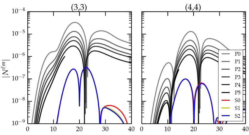
and PittNull CCE codes in the Bouncing BH test . . . 32 2.5 The absolute values of the News modes for the (3,3) and (4,4) for both the SpEC
and PittNull CCE codes in the Bouncing BH test . . . 33 2.6 The absolute values of the (2,2) News modes from our SpEC code for different
coordinate world tube radii ˘r in the Bouncing BH test . . . 36 2.7 The absolute values of the News modes for the (2,0) and (3,0) for both the SpEC
and PittNull CCE codes in the gauge wave test . . . 38 3.1 Phase difference between 1PN TaylorT4 tidal splicing and numerical waveforms . . 45 3.2 Phase difference between TaylorF2 tidal splicing and numerical waveforms . . . 48 3.3 Phase accumulation of 1PN Tidal effects . . . 49 4.1 The dynamical tides amplificationκ`as a function of orbital frequency . . . 64 4.2 Distribution of mismatches against the inspiral of the BHNS, q = 1, nonspinning
simulation across sky locations. . . 71 4.3 Distribution of mismatches against the inspiral of all numerical simulations . . . 72 4.4 Distribution of mismatches with only (2,±2) mode against the inspiral of all
LIST OF TABLES
Number Page
4.1 List of parameters for numerical simulations considered . . . 69 4.2 Universal Relations relating the static dimensionless deformability to various other
C h a p t e r 1
INTRODUCTION
One prediction of Einstein’s theory of General Relativity (GR) is the existance of gravitational waves, ripples of gravity propagating at the speed of light which very subtly distort the space they pass through. Similar to how accelerating electrons and protons emit electromagnetic radiation, a pair of massive objects orbiting around each other under the influence of gravity will emit gravi-tational radiation. The more massive the objects and the faster they are moving, the larger these ripples will be.
When two objects are orbiting each other in a binary, the emission of gravitational radiation will cause the orbits to slowly decay and the objects to orbit closer to each other. As the orbit shrinks, they orbit about each other faster, leading to a greater emission of gravitational radiation. If there are no other effects influencing the orbits, this process will continue, slowly accelerating the objects in the binary closer to each other until they collide, merging into a single object. The gravitational waves will be largest when a pair of ultra dense objects are orbiting in close proximity to each other. Thus, the binaries which will generate the strongest gravitational waves will be those comprising of either a Black Holes (BH) or a Neutron Stars (NS) during the last, decaying orbits as they coalesce into a single object.
For most of the past century, gravitational waves even from colliding BHs or NSs were far too weak for observatories on Earth to detect, as the source of those systems typically originate hundreds of millions or billions of light-years away. It has only been in the past few years, with the impressive developments with the aLIGO [2] and Virgo [14] detectors, has the technology improved to the point where these faint signals can be observed, opening a new window to peer at the rest of the universe. The first detection of colliding BHs, GW150914 [7] (named according to the date it was detected), heralded the start of gravitational wave astronomy. This direct detection of gravitational waves led to the 2017 Nobel Prize in Physics. There have since been a number of additional observations of the colliding BHs [6, 10–12], as well as a detection of colliding NSs, GW170817 [13]. As the detectors push to ever more sensitive configurations, the number of expected gravitiational wave signals they are expected to observe will only increase.
signals used to generate the template bank.
The primary difficulty of computing the possible gravitational waves to populate the template bank is that there are no closed form solutions to describing the orbits of a binary evolving according to GR. As such, researchers employ other methods to compute the theoretical signals, from numerical simulations to analytic approximants and calibrated models, each with their own advantages and disadvantages.
Numerical simulations are preferable, as they are the full calculation of the binary within GR using computational techniques. Current simulations of these binaries employ a "3+1" decompostion, where they compute the Einstein equations across 3 spatial dimension at a single time slice, then using those results in order to advance the simulations forward to the next discrete time slice. One limitation of this formulation is that such simulations only extend to a compact spatial region around binary and nowhere near the typically millions to billions of light-years of intervening distance be-tween the binary and detectors on Earth. While there are a few methods for estimating the resulting gravitational waves from the outer edge of the simulations, they are not perfect and the particular way in which the simulation chooses its coordinates can affect them.
These limitations led to the development of a method called Cauchy-Characteristic Extraction (CCE) [35, 36, 39], which can simulate how pattern of radiating gravitational waves propagate outward to arbitrarily far distances. It does so by way of a "2+1+1" decomposition of the Einstein equations, which evolves the spacetime along the trajectories of the gravitiational waves. While this method does not work for the intense, dyanmical gravity near compact orbiting objects, CCE can extract the results from the outer edge of the 3+1 simulation to compute the final signals which would be observable from Earth. This also means that we can use CCE in order to study how the local GR physics connect to measurable quantities by distant observers, such as measuring the ringdown [32], as well as kicks and fluxes of angular and linear momentum from merging binaries. While an older version of a finite-differencing CCE code has been available for use [21, 135, 136] it was only recently with the development of a spectral version of CCE which promised to be fast enough for large scale use. Chapter 2 includes detailed discussion of the numerous changes and improvements made to this spectral CCE code since its initial implementation in [87–89]. It also includes various tests of the code demonstrating its accuracy and efficiency in computing the radiated gravitational waves.
An alternative method of generating the signals from these binaries is analytic approximants which are cheap to generate while the orbit is decaying. Within these approximations, the NSs are treated as corrections to binaries comprised of only BHs. However, they are approximations so their accu-racy worsens as the objects near collision. Ironically, it is the corrections corresponding to the BH only system which are expected become inaccurate before the additional NS corrections fully man-ifest in the gravitational wave signal. In this sense, the analytic approximants for NSs in a binary are limited by the relatively poor knowledge of the BHs.
This particular dichotemy of relatively efficient simulations of BHs and cheap analytic corrections for NSs which gives rise to a hybrid method of generating gravitational wave signals for binaries with NSs that I have innovated called ‘Tidal Splicing’. This method works by treating the signal from the numerical simulations as if it had been generated as a corrected analytic approximant. Then the analytic corrections for the NSs are added on top of the numerical results, generating a new signal which approximates the orbital behavior as if the binary had been made of NSs originally. This also allows us to disentangle the contributions of individual effects, such as spinning NSs and dynamical tides, to the overall signal by tuning which effects we include when splicing the waveform. Chapters 3 and 4 give a full description of the concepts behind this model and results when compared with numerical simulations with NSs.
C h a p t e r 2
SPECTRAL CAUCHY-CHARACTERISTIC EXTRACTION
2.1 Introduction
The discovery of GW150914 [7] heralded the beginning of gravitational wave astronomy. In the subsequent years that detection has been followed up by a number of other signals observed from binary black hole (BBH) mergers [6, 10–12], as well as from the merger of a binary neutron star (BNS) system [13]. As the aLIGO [2] and Virgo [14] detectors push to ever greater sensitivities, the number of expected observations will continue to grow.
Extracting the signals from the noise involves matching the incoming data against a template bank of theoretically expected waveforms generated across possible binary configurations. The efficacy of extracting the configuration parameters (for instance, masses and spins of the binary components) from a given signal depends on the fidelity of the computed waveforms comprising the template bank; this is because errors in the template bank will bias the estimated parameters. The only ab initio method of generating accurate theoretical waveforms for merging BBH systems is via numerical relativity: the numerical solution of the full Einstein equations on a computer. Other methods of generating theoretical BBH waveforms, such as Effective One-Body solutions [53] and phenomenological models [101, 104], are calibrated to numerical relativity.
One limitation of numerical relativity simulations is that they all rely on a Cauchy approach in which the spacetime is decomposed into a foliation of spacelike slices, and the solution marches from one slice to the next. Such an approach can compute the solution to Einstein’s equations only in a region of spacetime with finite spatial and temporal extents bounded around the compact objects, whereas the gravitational radiation is defined at future null infinityI+. Extracting the waveform signal from the simulations with these finite extents requires additional work.
The most common method of extracting the gravitational radiation from a numerical relativity sim-ulation is to compute quantities such as the Newman-Penrose scalarΨ4[119] or the Regge-Wheeler and Zerilli scalars [140] at some large but finite distance from the near zone (perhaps 100–1000M, where M is the total mass of the system), typically on coordinate spheres of constant coordinate radiusr. Because these quantities or the methods of computing them include finite-radius effects, these quantities are computed on a series of shells at different radii r, fit to a polynomial in 1/r, and then extrapolated to infinity by reading offthe 1/r coefficient of the polynomial [57]. As the extraction surfaces are shells of constant coordinate radii, the choice of gauge implemented in the simulation can contaminate the resulting waveforms. Furthermore, if the shells are too close to the orbiting binary, the extrapolation procedure might not remove all of the near-zone effects.
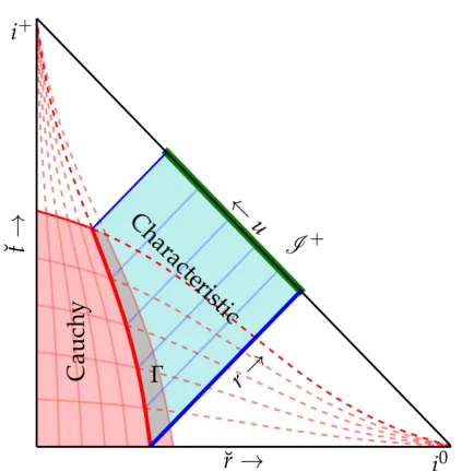
be measured. This can be done by rewriting Einstein’s equations using a characteristic formal-ism [54, 122, 139], in which the equations are solved on outgoing null surfaces that extend toI+. This formalism chooses coordinates that correspond to distinct outward propagating null rays, so it fails in the dynamical, strong field regime at any location where outgoing null rays intersect (i.e., caustics). Because of this, characteristic evolution is unable to evolve the near-field region of a merging binary system, so it cannot accomplish a BBH simulation on its own. However, it is possi-ble to combine an interior numerical relativity code that solves the equations on Cauchy slices with an exterior characteristic code that solves them on null slices; this approach is known as Cauchy-Characteristic Extraction (CCE). (See Fig. 2.1.)
Specifically, CCE takes metric data known on a world tubeΓ (thick red line in Fig. 2.1) that lies on or inside the boundary of a Cauchy evolution (red region), and treats it as inner boundary data for a characteristic evolution outward along null slices (blue curves). Because the combined CCE system uses the full Einstein equations, it produces the correct solution atI+, with the characteristic evolution properly resolving near-zone effects. The gravitational radiation is computed according to a particular inertial observer atI+(green curve). This particular observer is related to any other inertial observer by a single BMS transformation [139] (the group of Lorentz boosts, rotations, and supertranslations [138]), so up to this BMS transformation the waveform is independent of the gauge chosen by the Cauchy evolution.
The first code to implement CCE was the PittNull code [35, 36, 39]. Since its initial implementation there have been a number of improvements made, and the current iteration of that code utilizes stereographic angular coordinate patches, finite-differencing, and a null parallelogram scheme with fixed time steps for integrating in the null and time directions. Overall the code is second-order convergent with resolution [21, 135, 136]. Compared to waveforms computed from a Cauchy code by evaluatingΨ4at finite radii and extrapolating tor → ∞as described above, waveforms extracted via CCE using PittNull were shown to better remove gauge effects and to better resolve them= 0 memory modes [125, 134, 151].
Currently, PittNull requires thousands of CPU-hours to compute a waveform atI+given worldtube output from a typical Cauchy BBH simulation at multiple resolutions [87]. While that cost is smaller than the computational expense of the Cauchy simulation, it is still unwieldy, and is likely one reason that most Cauchy numerical-relativity codes do not use CCE despite the availability of PittNull. Because the metric in the characteristic region is smooth, the computational cost of characteristic evolution should be greatly reduced by using spectral methods instead of finite differencing. Such a spectral implementation of characteristic evolution has been introduced in the SpEC framework [87– 89]. Their tests showed improved speed and accuracy over the finite-difference implementation of PittNull [87, 88].
better handling of the inertial coordinates atI+. We demonstrate through a series of analytic tests that our version of CCE can compute waveforms with much lower computational cost than PittNull.
We start with a brief summary of the Bondi metric and the null formulation of the Einstein equations in Sec 2.2. A detailed explanation for how CCE works can be broken up into three distinct parts: the inner boundary formalism, the volume characteristic evolution, and theI+ extraction, which we describe in subsequent sections. Sec 2.3 describes the means by which the metric data known on a world tube is converted into Bondi form to serve as the inner boundary values for the characteristic evolution system. Sec 2.4 discusses the process of evolving Einstein’s equations from the inner boundary toI+. Sec 2.5 explains how to take the metric data computed on I+ and extract the Bondi news function in the frame of an inertial observer atI+. In Sec 2.6, we describe code tests and performance.
Throughout this paper, indices with Greek letters (µ, ν, ...) correspond to spacetime coordinates, lowercase Roman letters (i,j, ...) to spatial coordinates, and capitalized Roman letters (A,B, ...) to angular coordinates, and we choose a system of geometrized units (c = G = 1). For convenience, we have included a definitions key in appendix 2.7.
2.2 Summary of characteristic formulation
In the characteristic region (see Fig. 2.1), we adopt a coordinate system xµ = (u,r,xA), whereu is the coordinate labeling the outgoing null cones, r is an areal radial coordinate, and xA are the angular coordinates. Note that a surface of constant (u,xA) is an outgoing null ray parameterized byr; for this reason we sometimes callr a “radinull” coordinate. The metric can then be expressed in the Bondi-Sachs form [54, 139],
ds2=− e2β(1+rW)−r2hABUAUB
du2−2e2βdudr−2r2hABUBdudxA+r2hABdxAdxB,
(2.1)
whereW corresponds to the mass aspect,UA to the shift, β to the lapse, andhAB to the spherical
2-metric. The quantityhABhas the same determinant as the unit sphere metricqAB,|hAB|= |qAB|. An additional intermediate quantity,QA, is defined to reduce the evolution equations to a series of
1st order PDEs,
QA =r2e−2βhABU,rB. (2.2)
Instead of expressing the metric in terms of tensorial objects, we employ a complex dyad so that the metric components can be computed as spin-weighted scalars, and each of these scalars can be expanded in terms of Spin-Weighted Spherical Harmonics (SWSHes) of the appropriate spin weight; see Appendix 2.7 for details about SWSHes. The dyadqA has the following properties:
qAqA=0, (2.3)
If we defineqAB andqAB such that
qAB =
1
2(qAq¯B+q¯AqB), (2.5)
qACqC B =δAB, (2.6)
then
qA =qABqB. (2.7)
We express the metric coefficients and the quantityQA in terms of spin-weighted scalars J,K,U,
andQ, defined by
J =1 2hABq
AqB, (2.8)
K =1 2hABq
Aq¯B, (2.9)
U =qAUA, (2.10)
Q=QAqA. (2.11)
The determinant condition onhAB defines a relationship betweenJandKas
K = p1+JJ.¯ (2.12)
We introduce one more intermediate variableH, the time derivative ofJ along slices of constantr,
H = J,u|r=const (2.13)
Evaluating the components of the Einstein equationGµν =0 provides a system of equations for the quantities β,Q,U,W, andH:
β,r =Nβ, (2.14)
(r2Q),r =−r2( ¯ðJ+ðK),r +2r4ð(r−2β),r +NQ, (2.15)
U,r =r−2e2βQ+NU, (2.16)
(r2W),r =1
2e
2βR −1−eβ
ðð¯eβ+ 1
4r −2(r4(
ðU¯ +ð¯U)),r +NW, (2.17)
2(r H),r =((1+rW)(r J),r),r −r−1(r2ðU),r +2r−1eβð2eβ−(rW),rJ+NJ, (2.18)
where
R=2K−ðð¯K+ 1 2( ¯ð
2J+
ð2J)¯ + 1
4K( ¯ðJ¯ðJ−ð¯JðJ),¯ (2.19) andNβ,NW,NQ,NW,andNJ are the terms nonlinear inJand its derivatives, as according to [39].
The equations are presented in a useful hierarchical order: the right-hand side of the β equation involves only J and its spatial derivatives, the right-hand side of theQ equation involves only J and β and their spatial derivatives, and so on for the other equations. Therefore, given data for all quantities on the inner boundary as well as J on an initialu =constant null slice, we can integrate the series of equations in Eqs. (2.14)–(2.18) on that slice from the inner boundary tor =∞to obtain β,Q,U,W and thenH in sequence on that slice. Then, given H = J,u|r=const on that slice, we can integrate forward in time to obtainJon the next null slice.
2.3 Inner Boundary Formalism
The coordinates used to evolve Einstein’s equations in the Cauchy region (red area of Fig. 2.1) are generally different from the Bondi coordinates discussed in Section 2.2. The Cauchy coordinates are chosen to make the interior evolution proceed without encountering coordinate singularities; the procedure for choosing these coordinates is complicated and typically involves coordinates that are evolved along with the solution [26, 60, 112, 128, 141, 147]. Therefore, for CCE we must transform from arbitrary Cauchy coordinates to Bondi coordinates at the worldtube. Here, in the Cauchy region, for simplicity we assume Cartesian coordinates (˘t,x˘˘ı) in which the world tube hypersurface Γ(which is chosen by the Cauchy code) is a surface of constant ˘r, where ˘r = px˘2+y˘2+z˘2. We also define angular coordinates ˘xA˘ = ( ˘θ,φ) in the usual way from the Cartesian coordinates ˘˘ x˘ı. The world tube serves as the inner boundary of the characteristic domain (see Fig. 2.1). On this boundary, we assume that the interior Cauchy code provides the spatial 3-metricg˘ı˘, the shift β˘ı, and the lapse ˘α, along with the ˘r and ˘tderivatives of each of these quantities. Angular derivatives of these quantities are necessary as well; however, we can compute those numerically within the worldtube itself, so they need not be provideda priori.
Ref. [36] describes how to take the data provided by the interior Cauchy code and covert it into Bondi form (Eq. (2.1)) to extract the inner boundary values of the evolution quantities (J|Γ, β|Γ, . . .).
This section is primarily a summary of their results; however, we use different notation than Ref. [36].
Intermediate Null Coordinates
Our goal is to transform from the coordinates (˘t,x˘˘ı) into Bondi coordinates. It is simplest to proceed in two steps: the first step, described in this subsection, is to construct coordinates foliated by outgoing null geodesics. The second step, described in Section 2.3, will be to transform from these intermediate coordinates to Bondi coordinates.
We begin by constructing the null generator `µ˘, which involves the unit outward spatial vector normal to the world tube’s surface, sµ˘, and the unit timelike vector normal to a slice of constant ˘t, nµ˘:
sµ˘ =* . .
,
0, g˘ı˘x˘˘
q
g˘ı˘x˘ ˘ıx˘˘
+ / /
nµ˘ =1 ˘ α
1,−β˘ı. (2.21)
Eq. (2.20) depends on our simplifying assumption that the world tube is spherical in Cauchy coor-dinates, and can be generalized.From these, the null generator is
`µ˘ = nµ˘ +sµ˘ ˘
α−g˘ı˘β˘ıs˘. (2.22) The time derivatives of these vectors are
s,µ˘˘
t =
0, (−g˘ı˘+s˘ıs˘/2)sk˘g˘k,˘t˘
, (2.23)
n,µ˘˘
t =
1 ˘ α2
−α˘,t˘, α˘,˘tβ˘ı−α β˘ ˘ı,t˘
, (2.24)
`µ˘
,t˘= n,µ˘˘
t+s
˘
µ ,t˘+`
˘
µ
−α˘,t˘+g˘ı˘,˘tβ˘ıs˘+g˘ı˘β˘ı,t˘s˘+g˘ı˘β˘ıs,˘t˘
˘
α−g˘ı˘β˘ıs˘ . (2.25)
We will now construct a null coordinate system based on outgoing null geodesics generated by`µ˘. Letλbe an affine parameter along these geodesics such that the value ofλon the world tubeΓis λ|Γ = 0. We also define a null coordinate ¯uand angular coordinates ¯x
¯
A = ( ¯θ,φ) that obey ¯¯ u = t˘
and ¯xA¯ = x˘A˘on the world tube, and are constant along the outgoing null geodesic generated by`µ˘. Thus we have defined a new intermediate coordinate system, ¯xµ¯ = ( ¯u, λ,θ,¯ φ) and we will express¯ the metricgµ¯ν¯ in these intermediate coordinates.
To do this, we will need to write down the coordinate transformation from ˘xµ˘ to ¯xµ¯ in a neigh-borhood of the world tube, not just on the world tube itself, because we need derivatives of this transformation. In particular, we will need derivatives with respect to λ. The derivative of the metric componentsgµ˘ν˘ along the null direction simply is
gµ˘ν, λ˘ =`γ˘gµ˘ν,˘γ˘. (2.26) The evolution of the coordinates ˘xµ˘ along null geodesics implies that in a neighborhood of the world tube
˘
x, λµ˘ =`ν˘∂ν˘x˘µ˘ =`µ˘. (2.27)
Given the new coordinates ¯xµ¯, the metric components in these coordinates are
gµ¯ν¯ = ∂x˘α˘ ∂x¯µ¯
∂x˘β˘
∂x¯ν¯gα˘β˘. (2.28)
On the world tube,
∂x˘α˘ ∂x¯A¯ =
∂x˘˘ı ∂x¯A¯,
∂x˘˘ı
∂u¯ =0, (2.29)
where the term ∂x˘˘ı/∂x¯A¯ the standard Cartesian to spherical Jacobian. The above values of the Jacobians hold only on the world tube. In addition to the metric itself, we will also need first derivatives of the metric, including the derivative with respect toλ. This requires theλderivatives of the Jacobians evaluated on the world tube, which we represent here as
∂2x˘µ˘ ∂x¯A¯∂λ =
∂`µ˘ ∂x¯A¯ =`
˘
µ ,A¯, ∂2x˘µ˘
∂u∂λ¯ = ∂`µ˘
∂u¯ =` ˘
µ
,u¯, (2.30)
where we have made use of Eq. (2.27).
We are now ready to write out the metric in these intermediate coordinates by taking the expression in Eq. (2.28) and taking the appropriate derivatives,
guλ¯ =−1, gλ λ =gλA¯ =0,
gu¯u¯ =g˘tt˘, gu¯A¯ =
∂x˘˘ı ∂x¯A¯g˘ı˘t,
gA¯B¯ = ∂x˘˘ı ∂x¯A¯
∂x˘˘ ∂x¯B¯g˘ı˘,
gA¯B, λ¯ = ∂x˘˘ı ∂x¯A¯
∂x˘˘
∂x¯B¯g˘ı˘, λ+ `
˘
µ ,A¯
∂x˘˘ı ∂x¯B¯ +`
˘
µ ,B¯
∂x˘˘ı ∂x¯A¯
!
gµ˘˘ı,
gA¯B,¯ u¯ = ∂x˘˘ı ∂x¯A¯
∂x˘˘ ∂x¯B¯g˘ı˘,t˘,
gu¯A, λ¯ =`µ˘,A¯g˘tµ˘ + ∂x˘˘ı ∂x¯A¯
g˘ı˘t, λ+`µ˘,u¯g˘ı ˘µ
, (2.31)
and
gu¯u¯ =gu¯A¯ =0, guλ¯ =−1, gA¯B¯gB¯C¯ =δCA¯¯,
gλA¯ =gA¯B¯gu¯B¯, gλ λ =−gu¯u¯+gλ
¯
Ag
¯
uA¯,
gA¯B, λ¯ =−gA¯C¯gB¯D¯gC¯D, λ¯ , gλA, λ¯ =gA¯B¯ gu¯B, λ¯ −gλC¯gB¯C, λ¯
. (2.32)
Bondi Form of Metric
wherer is a surface area coordinate,u = u,¯ θ = θ, and¯ φ = φ. The surface area coordinate¯ r is defined by
r = |gAB| |qAB|
!14
= |gA¯B¯|
|qA¯B¯|
!14
, (2.33)
whereqA¯B¯ is the unit sphere metric.
The components of the metric in Bondi coordinates are then
gµν= ∂x
µ
∂x¯α¯ ∂xν
∂x¯β¯g ¯
αβ¯. (2.34)
The Jacobians include the derivatives of the Bondi radiusr. We compute
r, λ =r
4g ¯
AB¯g ¯
AB, λ¯ ,
r,u =r
4g ¯
AB¯g ¯
AB,¯u¯. (2.35)
Since the only difference between the Bondi and intermediate coordinates is the choice of radinull coordinates, the Jacobians for theu,θandφdirections are trivial. Eq. (2.32) gives us
guu =gu¯u¯ =0, gu A =gu¯A¯ =0,
gAB =gA¯B¯. (2.36)
The other metric components are
gur = ∂r ∂x¯µ¯g
¯
uµ¯ =−r
, λ,
gr r = ∂r ∂x¯µ¯
∂r ∂x¯ν¯g
¯
µν¯ = r
, λ2gλ λ+2r, λr,A¯gλ ¯
A−r ,u¯
+r,A¯r,B¯g ¯
AB¯,
gr A= ∂r ∂x¯µ¯g
¯
Aµ¯ =r
, λgλA¯ +r,B¯g ¯
AB¯. (2.37)
Becauseu and xA are equal to ˘t and ˘xA˘ on the world tube and are constant along outgoing null geodesics, the time and angular coordinates (˘t,x˘A˘) on the world tube determine the coordinates u and xA throughout the characteristic region, including on I+. Thus, the coordinates at I+ will be gauge-dependent, since ˘t and ¯xA¯ are dependent upon the gauge choices made in the 3+1 Cauchy evolution. We will later eliminate this gauge dependence by evolving and transforming to the coordinates of free-falling observers onI+, as described below in Sec. 2.5.
Inner Boundary Values of Characteristic Variables
Now that we have the full Bondi metric, we assemble the inner boundary values for the various evolution variables used in the volume,J, β,Q,U,W,andH. We write out the complex dyads as
qA= −1,− i sinθ
!
. (2.38)
Now because these complex dyads form the basis of the unit sphere metricqAB, and becauseqAB is indepedent of time and radius, along each ray these dyads are constant, thusqA, λ = qA, λ =0. Inverting the metric in Eq. (2.1),
gµν =
0 −e−2β 0A
−e−2β (1+rW)e−2β −e−2βUA
0B −e−2βUB r−2hAB
, (2.39)
wherehABhBC =δCA and|hAB| =|qAB|.
In the PittNull code, the quantities J, β, Q,U, andW and their λ derivatives are computed on the worldtube, and then J, β, Q, U, andW are extrapolated offthe worldtube onto a surface of constant Bondi radiusr [36]. PittNull then chooses its internal compactified radinull coordinates in the characteristic region to be surfaces of constantr.
However, in Ref. [87] and here, we avoid extrapolation, and we instead choose the worldtube to be at a constant value of our compactified radial coordinateρ,
ρ= r
R+r (2.40)
whereR(u,xA) =r|Γis the Bondi radius (Eq. (2.33)) of the world tube,
R=r|Γ (2.41)
Note thatRdepends onuandxAand thatρruns fromρ|Γ=1/2 to ρ|I+ =1. Because of our choice
of compactified radinull coordinate,Rand its derivatives evaluated on the world tube (Eq. (2.35)),
R, λ =r, λ|Γ, (2.42)
R,u =r,u|Γ, (2.43)
will appear in our equations, and we need to carefully distinguish between derivatives with respect touorxAat a constant value ofr(which appear in Eqs. (2.14)–(2.18)), and derivatives with respect touorxAat a constant value ofρ(which appear, e.g., in Eq. (2.43)).
We can now write down the inner boundary values of the characteristic variables in terms of the metric coefficients that we have computed at the inner boundary. Going back to the definition of J = 12qAqBhAB, we get the expressions
J|Γ =
1 2R2q
AqBg
AB, (2.44)
K|Γ =
q
1+J|ΓJ¯|Γ, (2.45)
J, λ|Γ =
1 2R2q
AqBg
AB, λ− 2R, λ
We can read offthe value forgur to compute β, β|Γ=−
1 2ln R, λ
.
(2.47)
We will also need β, λ|Γin order to computeQ|Γ. Directly differentiating Eq. (2.47) yields
β, λ|Γ =−
R, λ λ
2R, λ, (2.48)
but this involves the quantityR, λ λ, which appears to depend on second derivatives of the metric. So we instead compute β, λ|Γusing β’s evolution equation, Eq. (2.154):
β, λ|Γ=
R 8R, λ
J, λ|ΓJ¯, λ|Γ− K, λ|Γ2
, (2.49)
which involves only first derivatives.
The quantitiesUandW can similarly be read offfrom the metric:
U|Γ =
gr A
gurqA, (2.50)
W|Γ =
1 R −
gr r gur −1
!
. (2.51)
To getQ|Γ, we will also needU, λ|Γ, which we compute by differentiating the expression forU|Γand
using Eq. (2.48) to eliminateR, λ λ in favor of β, λ|Γ:
U, λ|Γ=− gλ
¯
A , λ+
R, λB¯
R, λ g
¯
AB¯ + R,B¯
R, λg
¯
AB¯
!
qA¯ +2β, λ|Γ
U|Γ+gλ
¯
Aq
¯
A
, (2.52)
where it is understood thatβ, λ|Γis to be evaluated using Eq. (2.49). Now that we have an expression
forU, λ|Γ, the inner boundary value ofQis given by
Q|Γ=R2
J|ΓU¯, λ|Γ+K|ΓU, λ|Γ
. (2.53)
The last quantity that we will need on the inner boundary is H = J,u|r=const. However, since the
worldtubeΓis not a surface of constantr, we must take care how we compute ouru-derivatives. In particular, differentiating Eq. (2.44) on the world tube gives us
J,u|Γ=
1 2R2q
AqBg AB,u−
2R,u
R J|Γ, (2.54)
where allu-derivatives are taken on the worldtube rather than holdingr fixed.
Note that the world tube is a surface of constantρ, our compactified radial coordinate. We introduce one last intermediate variableΦ= J,u|ρ=const, so we can write Eq. (2.54) as
Φ|Γ=
1 2R2q
AqBg
AB,u− 2R,u
Note that if the world tube is located at a fixed value of ˘r, as we assume here, the derivativesgAB,u
andR,u can be taken at constant ˘r. Instead, if the world tube is allowed to move freely (within the Cauchy ˘xα˘ coordinate system), then an additional correction factor depending on the worldtube’s coordinate velocity will be necessary to convertgAB,u|r˘=constandR,u|r˘=consttogAB,u|ΓandR,u|Γ.
To computeHin terms ofΦwe use Eq. (2.40):
H=Φ−ρ(1−ρ)R,u
R J, ρ. (2.56)
This formula will appear again in the volume evolution; see Sec 2.4. Since we have already com-puted J, λin Eq. (2.46), we convert J, ρtoJ, λ,
J, ρ=∂ ρ∂r ∂λ∂r J, λ = R
(1− ρ)2 1
r, λJ, λ. (2.57)
After substituting this into Eq. (2.56) and evaluating at the inner boundary (ρ = 1/2), the formula for the inner boundary value ofH is
H|Γ=Φ|Γ−
R,u
R, λJ, λ|Γ. (2.58)
Right now the information flow for the inner boundary formalism is entirely outgoing. That is, in-formation from the interior spacetime feeds into the CCE evolution, yet the CCE evolution does not feed back into the interior spacetime. An extention of CCE, called Cauchy-Characteristic Matching (CCM) [36] involves converting from the Bondi metric back into the world tube metric, coupling the information from the volume evolution back into the interior spacetime, effectively providing solu-tions to the boundary condition on the interior spacetime which fully satisfies the Einstein equasolu-tions. While a previous code has successfully performed CCM in the linearized case, they were unable to stabily run it for the general case [146]. Future work on our code will attempting to implement CCM in our code so that we can fully couple it to the evolution of the interior spacetime and bypass the need for separate boundary conditions for the Cauchy codes.
Computational Domain
2.4 Volume Evolution
Computational Domain
Because the domain of CCE extends all of the way out toI+where the Bondi radius is infinite, to expressI+on a finite computational domain, we define a compactified coordinate,ρ, in Eq. (2.40). This choice of compactification is subtly different from that which is used in PittNull [135]. Because they extrapolate quantities on the worldtube onto a hypersurface of constant Bondi radius, their compactification parameter is constant and unchanging during their entire evolution. By tying our compactification parameter to a fixed coordinate radius ˘r and allowing the Bondi radius to change freely, we must be careful in how we define our derivatives.
One consequence of utilizing ρis that angular derivatives computed numerically on our grid,ð|ρ, are at a constant value ofρ, so these are not the same as angular derivatives defined on surfaces of constantr, which we denote asð. Since Eqs. (2.14)–(2.18) involveðand notð|ρ, we must apply a correction factor to computeðfromð|ρ:
ðF =ð|ρF−F, ρð|ρρ=ð|ρF−F, ρ
ρ(1−ρ)
R ð|ρR, (2.59)
for an arbitrary quantityF. Similar correction factors are needed for second derivatives that appear in the evolution equations:
ðF, ρ=ð|ρF, ρ−F, ρ 1−2ρ
R ð|ρR−F, ρρ
ρ(1− ρ)
R ð|ρR, (2.60)
¯
ððF=ð¯|ρð|ρF+F, ρ
ρ(1−ρ) R2
!
2(1− ρ) ¯ð|ρRð|ρR−Rð¯|ρð|ρR
−ð|ρF, ρ
ρ(1− ρ) R ð¯|ρR
!
−ð¯|ρF, ρ
ρ(1−ρ) R ð|ρR
!
+F, ρρ ρ(1− ρ)
R
!2
¯
ð|ρRð|ρR. (2.61)
Correction factors for ¯ðF, ¯ðF, ρ,ððF,ðð¯F, and ¯ðð¯Fare obtained by appropriately interchangingð
and ¯ðin Eqs. (2.59)–(2.61).
Numerical derivatives with respect totanduare also taken at constantρon our grid, but at constant r in the equations, so similar correction factors are required there as well, as discussed below in Sec. 2.4.
We employ computational grid meshes suitable for spectral methods, Chebyshev-Gauss-Lobatto for the radinull direction andSpinsfastmesh for the angular directions.
Initial Data Slice
is ensuring the regularity of J atI+; the main physical consideration in typical applications is choosing a Jthat corresponds to no incoming radiation [21, 37].
We choose a piecewise function that takes the inner boundary valueJ|Γ and rolls it to J|I+ = 0 so
thatJon the initial slice is smooth through second radinull derivatives,
J =j0(ρ)J|Γ,
j0(ρ) =
1, ρ≤ ρ0,
10X3ρ−15Xρ4+6X5ρ, ρ0 ≤ ρ≤ ρ1,
0, ρ≥ ρ1,
Xρ = ρ1
−ρ0+ ρ1 − 1
−ρ0+ρ1ρ (2.62)
where Xρ has been chosen so that Xρ(ρ0) = 1 and Xρ(ρ1) = 0, and the polynomial j0(ρ) is determined by matching conditions at the interface of the piecewise function. Thus, J is second order smooth everywhere on the initial slice. We have currently set the bounds of this rollofffunction as (ρ0, ρ1)= (.55, .95).
Radinull Integration
The characteristic equations Eqs. (2.14)–(2.18) can be solved in sequence by integration inr from the worldtube to I+. We use a numerical radinull grid in the compactified variable ρ, and we re-express the characteristic equations in terms of ρ derivatives; see Eqs. (2.154)–(2.159). The grid points in ρare chosen at Chebyshev-Gauss-Lobatto quadrature points. The radinull equations for β, ρ andU, ρ (Eq. (2.154), (2.156)) both lend themselves to straightforward
Chebyshev-Gauss-Lobatto quadrature. Starting at the inner boundary values of β|Γ(Eq. (2.47)) andU|Γ (Eq. (2.51)),
these evolution variables are integrated out toI+.
A quick examination of the radinull equations for the evolution quantitiesQ, ρ,W, ρ,andH, ρ(Eq. (2.155), (2.158), (2.159)) reveals powers of (ρ−1) in denominators, so care must be taken to maintain reg-ularity atI+(where ρ = 1). A previous version of this same spectral CCE method [87] utilized integration by parts in order to rewrite the equations in a form without poles, allowing them to be integrated directly via Chebyshev-Gauss-Lobatto quadrature. However, integration by parts in-troduced logarithmic terms like log(1− ρ) which canceled analytically in the final expressions but which were not well represented by a Chebyshev-Gauss-Lobatto spectral expansion inρ. These log-arithmic terms spoiled exponential convergence and led to a large noise floor, limiting the accuracy of the method. We choose an alternative approach here.
The evolution equation forQ, Eq. (2.155), can be written in the form
(r2Q), ρ= QC
(1− ρ)2 + QD
(1− ρ)3, (2.63)
To better characterize the asymptotic behavior of this equation, we rewrite the system in terms of the inverse radinull coordinatex= R/r =1/ρ−1. Then Eq. (2.63) becomes
Q x2
!
,x
= C x2 +
D
x3, (2.64)
where
C =−QC+QD
R2 , (2.65)
D=−QD
R2 . (2.66)
We know the right-hand side quantitiesCandDare regular atx =0, and we seek a solutionQthat is also regular there. So we introduce new variables, motivated by Taylor series expansions ofQ,C, andDaboutI+(x=0),
Q=Q−Q|I+−xQ,x|I+, (2.67) C=C−C|I+−xC,x|I+, (2.68) D = D−D|I+−x D,x|I+−
x2
2 D,x x|I+. (2.69) Thus, by construction,QandCare both guaranteed to behave likex2near x =0 whileDbehaves asx3. Substituting these variables into Eq. (2.64) and gathering like terms, we find the differential equation
Q x2
!
,x
= C x2 +
D x3 +
2C,x|I++D,x x|I+
2x +
Q,x|I++C|I++D,x|I+
x2 +
2Q|I++D|I+
x3 . (2.70)
Because of how we have definedQ,CandD, any potential singularity issues are confined to the last three terms. To satisfy Eq. (2.70) for allx, the numerators of each of these terms must identically vanish, providing constraints and boundary conditions on the asymptotic values ofQ,C, andD,
Q|I+ =−D|I+
2 , (2.71)
Q,x|I+ =−C|I+−D,x|I+, (2.72) 0=−C,x|I+−
1
2D,x x|I+. (2.73) The last equation, Eq. (2.73) is a regularity condition onCandD. It turns out that this condition is guaranteed to be satisfied ifJ =0 andJ,x x=0 atI+.
We now integrate the equation
Q x2
!
,x
= C x2 +
D
x3 (2.74)
with inner boundary value
Q|Γ=Q|Γ+
D|I+
2 + C|I++D,x|I+
to obtainQat all radinull points. Then we reconstructQby adding back in its asymptotic values, Q=Q − D|I+
2 −x C|I++D,x|I+
.
(2.76)
Because the equation forQdoes not mix the real and imaginary parts ofQ, we follow [87] and solve for real and imaginary parts ofQseparately.
Examining the evolution equation forW, Eq. (2.158), we recognize that it has the same form as the equation forQ, Eq. (2.155). Therefore, in order to solve forW, we use the same procedure as we do forQ, following from Eq. (2.63) through Eq. (2.76) but replacing all of quantities specific toQ with theirW equivalents.
The radinull equation forH, Eq. (2.159) can be written as
(r H), ρ−r J(HT¯ −HT)¯ =HA+ HB 1−ρ +
HC
(1−ρ)2, (2.77) whereHB =ΣiHBi. The form of this equation is very similar to that of Eq. (2.63) that governs the Q(andW) radinull evolution. However, there is now the additional complication of whereby H, ρ
has a term proportional to not onlyH, but also to ¯H. This couples the real and imaginary parts of the equation.
The previous version of this code employed the Magnus expansion in order to handle this diffi-culty [87]. While the Magnus expansion might be useful for systems where the terms in its expan-sion are rapidly shrinking, there is no guarantee that will hold in general. Instead, we will write the system as a matrix differential equation, expressingH(andHA,HB,andHC) as column vectors like
H=* ,
<(H) =(H) +
-, (2.78)
and defining the quantityMas
M≡* ,
<(J)<(T) <(J)=(T) =(J)<(T) =(J)=(T) +
-, (2.79)
so thatM H here represents matrix multiplication. Then Eq.(2.77) becomes the matrix equation,
(r H), ρ−r M H =HA+
HB
1−ρ + HC
(1−ρ)2, (2.80)
As before, we convert from ρ into the inverse radinull coordinate x = R/r = 1/ρ−1 to better characterize its behavior nearI+,
H x
!
,x
+MH x = A+
B x +
C
x2 (2.81)
where
M= M
A=− HA
R(1+x)2, (2.83)
B=− HB
R(1+x), (2.84)
C=− HC
R . (2.85)
As we did with theQequation, we shall introduce one final set of variables, motivated by Taylor series expansions ofH,B,andCaboutx =0.
H =H−H|I+, (2.86)
B=B−B|I+− MH|I++M|I+H|I+, (2.87) C=C−C|I+−xC,x|I+. (2.88) Once again, these variables are constructed so thatH andBbehave asx andCbehaves asx2 in a neighborhood aboutx =0. Substituting these into Eq. (2.81), we get
H x
!
,x
+MH x =A+
B x +
C x2 +
H|I++C|I+
x2 +
B|I++C,x|I+− M|I+H|I+
x (2.89)
As before, the numerators of the last two terms must vanish, which gives us a boundary condition onHatI+,
H|I+ =−C|I+, (2.90)
and a boundary constraint onB,C, andM,
0= B|I++C,x|I++M|I+C|I+. (2.91) The last constraint is a regularity condition that is guaranteed to be satisfied if J =0 and J,x x = 0 atI+. We then integrate the equation
H x
!
,x
+MH x =A+
B x +
C
x2 (2.92)
from the worldtube toI+, with boundary valueH|Γ = H|Γ+C|I+, to obtainH on the entire null
slice. We reconstructHby computing
H=H −C|I+. (2.93)
To help ensure the stability of the system, we perform spectral filtering for each of the evolution quantitiesJ, β,Q,U,W, andHafter every time we compute them, similar to [87]. For the angular filtering, we set to 0 the highest two`−modes in the spectral decomposition on each shell of constant ρ. Thus, resolving the system up through`ma x modes requires storing and evolving the evolution
quantities in the volume up through`= `ma x+2 modes. We filter along the radinull direction by
taking the spectral expansion of the evolution quantities along each null ray and scaling thei−th coefficient by
e−108(i/(nρ−1))16, (2.94)
Time Evolution
To evolveJforward in time, we integrate
J,u|ρ=const=Φ (2.95)
at each radinull point using the method of lines. This is done using an ODE integrator, integrating forward inu, with a supplied right-hand-sideΦ. HereΦis computed using
Φ= H+ρ(1− ρ)J, ρ
R R,u, (2.96)
(see Eq. (2.56)), whereHis the result of the radinull integration, Eq. (2.18), accomplished using the method in Section 2.4.
The time integration of J (Eq. (2.95)) uses a 5th order Dormand-Prince ODE solver with adaptive timestepping [126], and a default relative error tolerance of 10−8 except where otherwise noted. Because this is a characteristic evolution, where each time step corresponds to a lightlike rather than spacelike slicing, there is no CFL condition on the size of the time steps. Thus, the step sizes are limited entirely by the error measure. The time evolution is also done in tandem with the evolution of the inertial coordinates (Eqs. (2.123)–(2.125)), and of the conformal factor (Eq. (2.107)) from scri extraction, as described below.
2.5 Scri Extraction
Once the characteristic equations have been solved in the volume so that the Bondi metric variables are known onI+, the gravitational waveform can be computed. This involves two steps. The first step is computing the Bondi News function at I+ from the metric variables there. The second step involves transforming the News to a freely-falling coordinate system atI+; this removes all remaining gauge freedom up to a BMS transformation. These steps are described below.
News Function
The Bondi metric given in Eq. (2.1) is divergent atI+wherer → ∞, so we work with a conformally-rescaled Bondi metric, ˆgµν = `2gµν, where` = 1/r, that is finite atr → ∞and which takes the form [35]
ˆ
gµν=−e2β(`2+`W)−hABUAUB
du2+2e2βdud`−2hABUBdudxA+hABdxAdxB.
(2.97)
HerehAB, β,W, andUAare the same quantities that appear in Eq. (2.1).
To facilitate the computation of the News function, we construct an additional conformal metric
˜
gµν =ω2gˆµν, (2.98)
that is inertial and asymptotically Minkowski atI+. The conformal factorω is chosen so that the angular part of ˜gµν is a unit sphere metric [149],
In terms of the original metric,
˜
gµν=Ωgµν, (2.100)
Ω=ω`. (2.101)
On a given constantu slice,ω can be computed by solving an elliptic equation related to the 2D curvature scalar,
R=2ω2+h|ABI+DADBlnω
, (2.102)
whereDAis the covariant derivative associated withhAB|I+. Expanding out the covariant derivatives
yields [35],
h|ABI+DADBlnω =
1 4
−2ð2lnωJ¯−2¯ð2lnωJ+4¯ððlnωK−ðlnωðJJ¯2−ðlnωðJ J¯ J¯
−2ðlnωðJ¯+2ðlnωðKJ K¯ +ðlnωð¯JJ K¯ +ðlnωð¯J J K¯ −2ðlnωð¯K JJ¯
+ðJð¯lnωJ K¯ +ðJ¯ð¯lnωJ K−2ðKð¯lnωJJ¯−ð¯lnωð¯J JJ¯
−2¯ðlnωð¯J−ð¯lnωð¯J J¯ 2+2¯ðlnωð¯K J K
, (2.103)
Eq. (2.102) could in principle be used to solve forωat each slice of constantu. However, we instead solve this equation forω only on the initial slice, where the equation simplifies significantly (see below), and then we construct an evolution equation forωand we evolveωas a function ofu. Note that when evolvingω, one could use Eq. (2.102) as a check to monitor the error inω; however we do not yet do so.
On the initial slice, Eqs. (2.102) and (2.103) simplify considerably; we have set J|I+ = 0 (see Eq. (2.62)), so Eq. (2.103) implies that hAB|I+DADBlnω = 4¯ððlnω and Eq. (2.19) implies that
R =2, reducing Eq. (2.102) to 1=ω2+ðð¯ lnω. This has the trivial solution ofω=1.
To derive an evolution equation forω, we instead turn to the generators atI+[35],
˜
nµ =g˜µν∇νΩ|I+, (2.104) ˆ
nµ =gˆµν∇ν`|I+ =gˆµ`, (2.105) so that
˜
nµ =ω−1nˆµ. (2.106)
Derivation for evolution of the conformal factor onI+in the frame of the compactified metric, is given in Ref [35], and can be computed by,
2 ˆnµ∇µlnω =−e−2βW|I+. (2.107)
original expression in the axisymmetric case [54]). Here we’ve factored the si slightly differently
then they did,
N = 1
16ωA(K+1) 4s1+2s2+
ðU¯ +ð¯U
s3− 8 ω2s4+
2 ωs5
!
, (2.108)
A=ωe2β, (2.109)
s1 =J2H¯,`+JJ H¯ ,`+2(K+1) H,`− J K,u`, (2.110) s2 =ðJ,`JJ¯U¯ +ðJ¯,`J2U¯ +2ðU JJ K¯ ,`+2ðU J¯ J J¯ ,`+ð¯J,`JJU¯ +ð¯J¯,`J2U+2¯ðU J2J¯,`+2¯ðU J¯ 2K,`
+(K+1)2ðJ`U¯ −2ðK,`JU¯ −2ðU JJ¯,`+4ðU K,`−2ðU J K¯ ,`+4ðU J¯ ,`+2¯ðJ,`U−2¯ðK,`JU
−2¯ðU J K,`−2¯ðU J J¯ ,`, (2.111)
s3 =J2J¯,`+JJ J¯ ,`+2(K+1)(J,`− J K,`), (2.112) s4 =ðAðωJJ¯+ð¯Að¯ωJ2+(K+1)
2ðAðω−ðAð¯ωJ−ð¯AðωJ
, (2.113)
s5 =2ð2AJJ¯+2¯ð2AJ2+ðAðJ JJ¯2+ðAðJ J¯ 2J¯−ðAð¯J JJ K¯ −ðAð¯J J¯ 2K+2ðAð¯K J2J¯
+2¯ðAðK J2J¯+ð¯Að¯J J2J¯+ð¯Að¯J J¯ 3−2¯ðAð¯K J2K
+(K+1)4ð2A−4¯ððAJ+2ðAðJJ¯+2ðAðJ J¯ −4ðAðK+2ðAð¯J−2¯ðAðJ+4¯ðAðK J
+(K+2)−2ðAðK JJ¯−ð¯AðJ JJ¯−ð¯AðJ J¯ 2
. (2.114)
The news as defined in Eq. (2.108) has spin-weight+2. However, the usual convention for gravi-tational radiation is to work with quantities with spin-weight−2. Furthermore, the news N has the opposite sign as the usual convention. By relating the News function computed here to the News function from the more typical Newman-Penrose formalism [119] (see Ref [23], in particular the discussion of computingΨ), we note that
NN-P=−2NCCE, (2.115)
where the quantity on the left is the usual definition and the quantity on the right is the one in Eq. (2.108).
Inertial Coordinates
Once the News function is computed according to Section 2.5, it is known as a function of coor-dinates (u,xA) on I+. Recall that these coordinates are chosen so that u = t˘and xA = x˘A˘ on the world tube, where (˘t,x˘A˘) are the time and angular coordinates of the interior Cauchy evolution. Therefore, the News as computed above depends on the choice of Cauchy coordinates.
On the initial slice, we choose ˜u=uand ˜xA˜ = xA. These inertial coordinates then evolve along the I+generators [35],
ˆ
nµ∂µu˜=ω, (2.116)
ˆ
nµ∂µx˜A˜ =0, (2.117)
where the ˆnµare given by elements of the compactified metric according to Eq. (2.105).
Since ˜xA˜ = ( ˜θ,φ) are not representable via a spectral expansion in spherical harmonics, thus making˜ them poor choices for our numerics, we represent the inertial coordinates using a Cartesian basis
˜
x˜ı=( ˜x,y,˜ z). We reexpand Eq. (2.117), using the transformations,˜ ∂θ˜
∂xµ =
1 ˜
x2+y˜2 −y˜ ∂x˜ ∂xµ +x˜
∂y˜ ∂xµ
!
, (2.118)
∂φ˜ ∂xµ =
1 ˜
r2px˜2+y˜2 x˜z˜ ∂x˜ ∂xµ +y˜z˜
∂y˜ ∂xµ −( ˜x
2+y˜2) ∂z˜ ∂xµ
!
. (2.119)
Plugging those into Eq. (2.117) yields the coupled equations
−y˜∂x˜ ∂u +x˜
∂y˜ ∂u =
ˆ nθ ˆ nu −y˜
∂x˜ ∂θ +x˜
∂y˜ ∂θ
!
+ nˆφ ˆ nu ∂ ∂θ → ∂ ∂φ ! , (2.120) ˜ xz˜∂x˜
∂u +y˜z˜ ∂y˜ ∂u −( ˜x
2+y˜2)∂z˜ ∂u =
ˆ nθ ˆ nu x˜z˜
∂x˜ ∂θ +y˜z˜
∂y˜
∂θ −( ˜x2+y˜2) ∂z˜ ∂θ
!
+ nˆφ ˆ nu ∂ ∂θ → ∂ ∂φ ! . (2.121)
By expanding the basis from 2 coordinates to 3, we also need to introduce a constraint which will force the ˜x˜ı to remain on the unit sphere and eliminate the extra degree of freedom, ˜r =
p
˜
x2+y˜2+z˜2 = 1. While this holds analytically, numerically ˜r will shift away from 1 during the evolution, which makes it necessary to introduce a constraint equation to the system of equations,
∂r˜ ∂u =x˜
∂x˜ ∂u +y˜
∂y˜ ∂u +z˜
∂z˜
∂u =rC˜ ( ˜r), (2.122) whereC( ˜r) is an constraint term whereC( ˜r = 1) = 0. In our code, C( ˜r) = −κ( ˜r −1) for some positive parameterκ.
With these three equations, Eqs. (2.120)–(2.122), we solve for the three ∂∂ux˜˜ı. After some manipula-tions and massaging, we obtain the evolution equamanipula-tions for the Cartesian inertial coordinates with respect to the characteristic coordinates,
∂x˜ ∂u =
˜ x ˜ rC( ˜r)+
1 ˜ r2 " ˆ nθ ˆ nu ( ˜r
2−x˜2)∂x˜ ∂θ −x˜y˜
∂y˜ ∂θ −x˜z˜
∂z˜ ∂θ
!
+ nˆφ ˆ nu ∂ ∂θ → ∂ ∂φ !# , (2.123)
∂y˜ ∂u =
˜ y ˜ rC( ˜r)+
1 ˜ r2 " ˆ nθ ˆ nu −x˜y˜
∂x˜
∂θ +( ˜r2−y˜2) ∂y˜ ∂θ −y˜z˜
∂z˜ ∂θ
!
+ nˆφ ˆ nu ∂ ∂θ → ∂ ∂φ !# , (2.124)
∂z˜ ∂u =
˜ z ˜ rC( ˜r)+
1 ˜ r2 " ˆ nθ ˆ nu −x˜z˜
∂x˜ ∂θ −y˜z˜
∂y˜
∂θ +( ˜r2−z˜2) ∂z˜ ∂θ
!
+ nˆφ ˆ nu ∂ ∂θ → ∂ ∂φ !# . (2.125)
is interpolated in time onto slices of constant ˜u, so that we then have both ˜xi˜( ˜u,xA) andN( ˜u,xA) = N( ˜u,x˜˜ı), using a cubic spline along each grid point onI+.
Then on each constant ˜uslice, we perform the spatial interpolation by projecting the News function onto its spectral coefficientsc`m, using the orthonormality of SWSHes from Eq. (2.153),
c`m( ˜u) =
Z
S2
N( ˜u,x˜˜ı)2Y`m( ˜θ,φ) sin ˜˜ θdθd˜ φ.˜ (2.126)
However, since we numerically evaluate News function on the computational grid corresponding to the characteristic coordinates, we must instead do the integration over its area elements, sinθdθdφ, so we convert the coordinates of this expression, which introduces the determinant of a Jacobian,
dθd˜ φ˜= dθdφ
∂x˜A˜ ∂xA . (2.127)
Once again, because of the difficulties of representing angular coordinates spectrally, we convert this expression from ˜θ and ˜φto ˜x˜ı. To facilitate our expansion to Cartesian coordinates, we introduce a temporary radial coordinates ˜randron the unit sphere with ˜xA˜ =(˜r,θ,˜ φ) and˜ xA = (r, θ, φ) so that we can properly define the determinants (keeping in mind ˜randrare analytically identical to 1 so will disappear from the final expressions),
∂x˜A˜ ∂xA =
∂x˜A˜ ∂x˜˜ı
∂x˜˜ı ∂xA = 1 ˜ r2sin ˜θ
!
∂x˜˜ı ∂xA . (2.128)
Plugging everything in yields the full expression,
c`m( ˜u)=
Z
S2
N( ˜u,x˜˜ı)2Y`m( ˜θ,φ)˜ 1 sinθ
∂x˜˜ı ∂xA
sinθdθdφ. (2.129)
Note that we have included a factor of sinθ/sinθ which, while analytically trivial, aids with the numerics of our code. Incorporating the sinθin the numerator generates the proper spherical area element for the integration, while we factor the 1/sinθinto the ∂φ∂ terms in the Jacobian, as numer-ically computed spherical gradients return factors ofsin1θ∂φ∂ .
If we want to convert these coefficients to the convention consistent with the Newman-Penrose notation, we must apply one last change according to Eq. (2.115),
c`mN-P=2(−1)1−mcCCE`−m. (2.130)
we have taken to representing the scri extraction portion at a significantly higher angular resolution from the rest of our code. In particular, when we properly resolve the volume evolution up to`ma x
angular modes, the use maintain a basis consisting of 2`ma x angular modes for our scri extraction
code. Our properly resolved information content is still no better than what is resolved in the volume evolution (i.e. `ma x), but this allows us to accurately project onto the inertial coordinates
with Eq. (2.129). Because the scri extration portion of the code is only a 2D surface, this choice is an insignificant contribution to the overall computational cost of our code.
While this coordinate evolution projects the News function on an inertial frame, it is not a unique inertial frame. The class of inertial observers atI+are all related to each other by the group of BMS transformations. Because our CCE inertial coordinates atI+correspond to free falling observers, the BMS frame remains constant throughout the entire characteristic evolution. Thus, the BMS frame we use in our evolution is frozen in entirely by our choice to identify our inertial coordinates with the characteristic coordinates on our initial slice (i.e. u˜ = u and ˜xA˜ = xA). This choice is in some sense arbitrary, as it is ultimately related to the coordinates provided on the world tube by the Cauchy evolution on that initial slice, and there no guarentee of consistancy between CCE evolutions on different world tubes even from the same Cauchy evolution. However, development of a consistent treatment of handing the choice of BMS frame is beyond the scope of this paper.
Computational Grid
We useSpherepackfor most of the Scri Extraction, with the final projection onto the inertial coor-dinates done usingSpinsfast. The time evolution of the inertial coordinates, Eqs. (2.123)–(2.125), and of the conformal factor, Eq. (2.107), is done in tandem with the evolution of J, Eq. (2.96), in the Volume Extraction, using the same routine (5th order Dormand-Prince) and error tolerance as specified for that evolution.
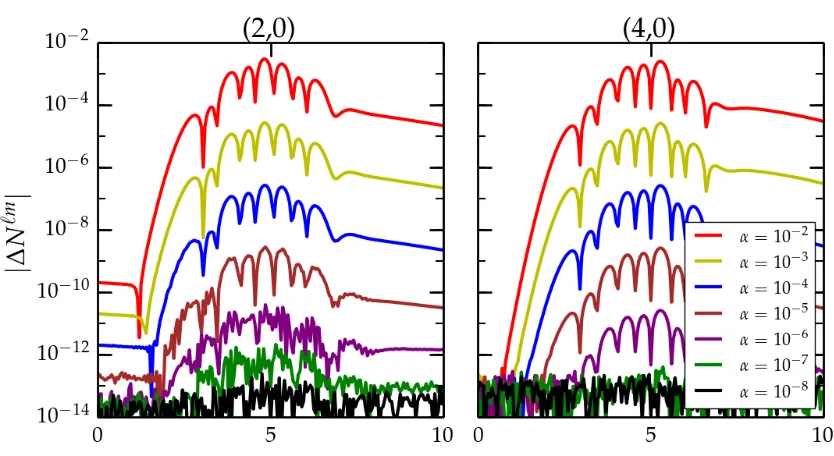
2.6 Code Tests
In order to showcase the accuracy, speed, and robustness of this spectral CCE code, we perform a number of tests on the code. We have two linearlized solutions, a trival analytic solution, and two fully nonlinear tests which outline how well the code can remove purely coordinate effects from the News output.
Linearized Analytic Solution
The linearized form for the Bondi-Sachs metric for a shell of outgoing perturbations on a Minkowski background was given in [38], though our choice of notation follows more closely with that used in [136]. We can express the solutions in terms of the metric quantities
Jl i n=p(`+2)!/(`−2)!2Z`m<J`(r)eiνu, Ul i n=p`(`+1)1Z`m<U`(r)eiνu,
βl i n=0Z`m<
Wl i n=0Z`m<W`(r)eiνu, (2.131) where ν is a real constant setting the frequency of the perturbations and J`(r),U`(r), β`(r) and W`(r) are all analytic complex functions of just the radius and `−mode of the perturbation, given below. The angular content is expressed through the varioussZ`m, which are just linear combina-tions of the typical SWSHes defined as in [38]
sZ`m =√1
2
s
Y`m+(−1)m sY`−m form>0,
sZ`m =√i
2
(−1)m sY`m− sY`−m form<0,
sZ`0 =sY`0. (2.132)
To get the linearized expression for Hl i n, we can simply take a directu derivative of Jl i n. Since
these expressions are defined according to the Bondi metric, with the Bondi radial coordinater (rather thanρ),uderivatives are taken along curves of constantr. ThusHl i n= Jl i n,u.
From this, the linearized News function can be expressed as
Nl i n =< eiνu lim r→∞
`(`+1) 4 J`−
iνr2 2 J`,r
!
+eiνuβ`
! s(`+
2)! (`−2)!
2Z`m. (2.133)
Ref [136] explicitly wrote out the solutions to the linearized evolution quantities and News function for the`=2 and`=3 modes, which we reproduce here. For`=2,
β2=B2,
J2(r)=24B2+3iνC2a−iν 3C
2b
36 +
C2a 4r −
C2b 12r3,
U2(r)=−24iνB2+3ν 2C
2a−ν4C2b
36 +
2B2 r +
C2a
2r2 + iνC2b
3r3 + C2b
4r4,
W2(r)=24iνB2−3ν 2C
2a+ν4C2b
6 +
3iνC2a−6B2−iν3C2b
3r −
ν2C 2b
r2 + iνC2b
r3 + C2b
2r4,
N2m=< iν 3C 2b √ 24 eiνu !
2Z2m, (2.134)
and for`=3, β3=B3, J3(r) =
60B3+3iνC3a+ν4C3b
180 +
C3a
10r − iνC3b
6r3 − C3b
4r4,
U3(r) =
−60iνB3+3ν2C3a−iν5C3b
180 +
2B3 r +
C3a
2r2 − 2ν2C
3b
3r3 +
5iνC3b
4r4 + C3b
r5 ,
W3(r) =
60iνB3−3ν2C3a+iν5C3b
15 +
iνC3a−2B3+ν4C3b
3r
−2iν 3C
3b
r2 − 4iν2C
3b
r3 + 5νC3b
2r4 + 3C3b
N3m =< −ν 4C
3b
√ 30
eiνu
!
2Z3m, (2.135)
where B`,C`a andC`b are all freely chosen complex constants. Note that only the values ofC`b
show up in the expression for the News.
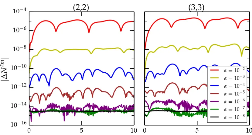
For the tests we performed here, we follow a similar setup as in [135, 136], where we evolve a system which is a simple linear combination of the (2,2) and (3,3) modes. Specifically, the parameter values are ν = 1, B` = .5iα,C`a = 1.5α, andC2b = −iC3b = .5α, where the constant αsets the
amplitude of the resulting News as well as the scale of the linearity of the system. Because we evolve the entire nonlinear solution, and not just a linearized version, we expect our results to differ from the analytic solution with differences that scale as the square of the amplitude,α2.
We place these linearized values of the evolution quantities (J,W,U, β) on a chosen world tube to serve as the inner boundary values for the volume evolution. By starting with the world tube in the Bondi metric, we bypass the entire inner boundary formalism since we are already starting with the Bondi metric quantities. To make this test even more demanding, we chose our world tube such that its Bondi radius varies both in time and across the surface, given by the formula
R=5 1+ (−.42x+.29y+.09z)(.2x+.1y−.12z)(.7x+.1y−.3z)(.12x−.31y−.5z) (x2+y2+z2)2 sinπu
!
.
(2.136)
We chose this distortion of the Bondi radius somewhat arbitrarily, ensuring that it had distortions with modes up through` = 4 as well as a time varying component with a frequency distinct from that of the linearized perturbation. This tests the code’s ability to distinguish betweenHandΦwith a correct handling of the moving world tube Bondi radius,R, at least to linear order. Since this test bypasses the inner boundary formalism, we can not make any claim about whether the coordinate radius ˘r of the world tube is moving as there is no defined coordinate radius.
The data for J on the initial slice we also read offfrom Eq. (2.131). With the world tube metric values and initial slice established, we evolve the full characteristic system. We resolve SWSH modes through ` = 8 with a radinull resolution of 20 grid points and relative time integration error tolerance of 10−8. We test the characteristic evolution against perturbation amplitudes of α = (10−2,10−3,10−4,10−5,10−6,10−7,10−8) from u = 0 to u = 10. We compute the difference between the computed News and the analytic results from Eq. (2.133),|∆N`m|= |NChar`m − Nl i n`m|in Fig 2.2. Note, we are examining the News function evalutated at theI+coordinates (u, θ, φ), rather than the inertial coordinates, ( ˜u,θ,˜ φ) because we expect the di˜ fference between the two systems to be a small correction to the linearized values.