MUTUAL INFORMATION AND THE DESIGN AND ANALYSIS OF RADAR WAVEFORMS AND SYSTEMS
Thesis by Mark Robert Bell
In Partial Fulfillment of the Requirements for the Degree of
Doctor of Philosophy
California Institute of Technology Pasadena, California
1988
11
-©
1988Mark Robert Bell
ACKNOWLEDGE:rv.IBNTS
I wish to thank my thesis advisor, Dr. Edward C. Posner, for his insightful guidance, discussions, and reviews of my work throughout the course of this research. His comments and questions have made this work both clearer and more relevant. I have been very fortunate to have an advisor with both the depth and breadth of knowledge that he possesses.
I also wish to thank the professors who make up my thesis committee, Dr. Yaser Abu-Mostafa, Dr. Charles Elachi, Dr. Joel N. Franklin, and Dr. Robert J. McEliece, for both taking the time to be on my committee and offering the excellent courses I have had the priviledge of taking with each of them.
I also thank Hughes Aircraft Company for sponsormg this work through a Howard Hughes Doctoral Fellowship.
- lV
-ABSTRACT
TABLE OF CONTENTS
ACKNOWLEDGEMENTS ... iii
ABSTRACT ... iv
LIST OF ILLUSTRATIONS ... ix
LIST OF TABLES ... xiii
CHAPTER 1. INTRODUCTION ... 1
1.1 Background ... 1
1.2 Overview ... 7
1.3 Chapter 1 References ... 10
CHAPTER 2. THE INFORMATION-THEORETIC ANALYSIS OF RADAR .. 11
2.1 The Information-theoretic Analysis of Radar Systems ... 12
2.2 Information Theory and Discrete Random Variables ... 22
2.3 Information Theory and Continuous Random Variables ... 37
2.4 Mutual Information and Radar Measurement Performance ... 45
- Vl
-CHAPTER 3. THE RADAR/INFORMATION THEORY PROBLEM ... 54
3.1 General Formulation of the Radar/Information Theory Problem ... 55
3.2 The Radar/Information Theory Problem for Discrete Target Channels ... 58
3.2.1 Solution for Discrete Memoryless Target Channels ... 60
3.2.2 The Radar/Information Theory Problem for N Observations of a Fixed Target ... 76
3.2.3 The Radar/Information Theory Problem for Finite-State Target Channels 79 3.3 The Radar/Information Theory Problem for Continuous Target Channels .. 95
3.3.1 The Continuous Memoryless Target Channel ... 97
3.4 Conclusions ... 103
3.5 Chapter 3 References ... 104
CHAPTER 4. RADAR SCATTERING MODELS ... 105
4.1 Radar Reflectivity and Radar Cross Section ... 106
4.2 The Analytic Signal Representation ... 112
4.3 Polarization, Depolarization, and Scattering ... 114
4.4 Statistical Models of Radar Backscatter from Land ... 118
4.5 A Model for Cross Polarization Measurements from Rough Surfaces ... 126
4.6 Spatial Resolution Characteristics of Radar vVaveforms ... 128
CHAPTER 5. MATCHING A RADAR WAVEFORM/RECEIVER-FILTER PAIR TO A TARGET OF KNOWN IMPULSE RESPONSE ... 148 5.1 Radar Target Detection by Energy Threshold Test ... 149 5.2 Matching a Waveform/Receiver-Filter Pair to a Target of Known
Impulse Response ... 156 5.3 Optimum Waveform/Receiver-Filter Pairs for Sphere Detection ... 170 5.4 Chapter 5 References ... 182
CHAPTER 6. INFORMATION THEORY AND RADAR WAVEFORM
DESIGN ... 183 6.1 Radar Waveform Design for Maximum Information Transfer
Between the Target and the Received Radar Signal ... 184 6.2 A Numerical Example ... 213 6.3 Radar Waveform Design and Implementation ... 228 6.4 Comparison of Waveforms for Optimum Detection and Ma."{imum
Vlll
-CHAPTER INFORMATION CONTENT OF RADAR IMAGES ... 237
7.1 Radar Images ... 238
7.2 Information Theory and Speckle Noise in Radar Images ... 259
7.3 Chapter 7 Appendix ... 276
7.3.1 Verification of Eq. (7.48) ... 276
7.3.2 Verification of Eq. (7.49) ... 277
7 .3.3 Verification of Eq. (7.54) ... 279
7 .4 Chapter 7 References ... 283
Figure
Page1.1. Block Diagram of a Generic Radar System ... 2
2.1. Block Diagram of a Generic Communication System ... 13
2.2. Block Diagram of a Generic Radar System ... 16
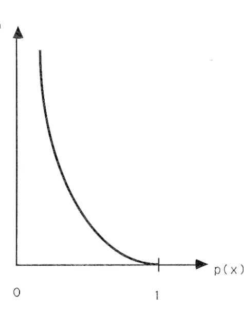
2.3. Self Information I(x) versus p(x) ... 23
2.4. Block Diagram of a Simple Communication System ... 31
2.5. Binary Symmetric Channel ... 32
2.6. The Binary Entropy Function 1-l((J) ... 34
2.7. Additive Gaussian Noise Channel ... .41
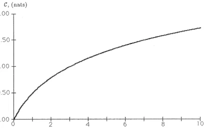
2.8. Capacity of the Additive Gaussian Noise Channel ... 44
2.9. Block Diagram of a Measurement System ... 45
2.10. Rate Distortion Function of the Gaussian Measurement Example ... .45
3.1. Block Diagram of Radar/Information Theory Problem ... 56
3.2. Block Diagram of The Target Channel ... 57
3.3. Radar/Information Theory Problem for Discrete Target Channels ... 59
3.4. Diagram of Target Channel for N
=
1 andX=
<Xj ••••••••••••••••••••• 61 3.5. Memoryless Binary Target Channel of Example 3.1 ... 65
-x-Page
3 Memoryless Discrete Target Channel of ....,,,.,_ .... ,.., ... 70
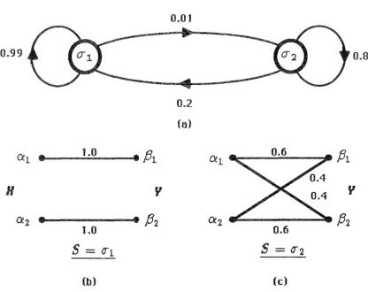
3.8. Finite-State Target Channel of Example 3.5 ... 83
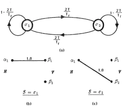
3.9. Finite-State Target Channel of Example 3.6 ... 84
10. Radar/Information Theory Problem for Continuous Target Channels ... 96
3.11. Continuous Target Channel Model ... 99
4.1. Waveform Spectra X(f) and R(f) ... 130
4.2. Constructive Interference from Two Scatterers ... 132
4.2. Two-Frequency Constructive Interference from Two-Scatterers ... 132
4.3. Single-Frequency Constructive Interference from Two-Scatterers ... 134
4.4. Radar Measurement of a Rough Surface ... 134
4.5. Constructive Interference and Waveform Bandwidth ... 139
4.6. Coordinate System of Scattering Problem ... 142
4.7. Linear Time-Invariant System Representation of Stationary Target-Scattering Mechanism ... 142
4.8. Continuous Spectra X(f) and R(/) of Radar Waveform ... 142
5.1. Probability Density Functions
/(elHo)
and/(elH1 ) . . • . . .
1525.2. Block Diagram of Radar Waveform/Receiver-Filter Design Problem ... 157
5.3. Linear System Representation of the Relation Between Q(f) and X(f) ... 163
5.5. Magnitude-Squared Spectrum JH(/) J2 versus
f ...
1735.6. Wave shape of
i(i)
for = 1 ... 1775 Wave shape of
x(i)
for T=
25 ... 1775.8. Wave shape of
i(-t)
for T=
50 ... 1785.9. Wave shape of £(1) for T
=
100 ... 1786.1. Block Diagram of The Radar Target Channel ... 185
6.2.
E(
a) as a function of a=T /W ...
1906.3. Additive Gaussian Noise Channel. ... 193
6.4. Another Interpretation the of Radar Target Channel ... 206
6.5. "Water-Filling Interpretation of IX(f)J2 •••••••••••••••••••••••••••••• 210 6.6. Example illustrating the resulting IX(/) 1 2 for a given
crb (/)
and P1111 ( / ) • • • • • • • • • • • • • • • • • • • • • • • • • • • • • • • • • • • • • • • • • • • • • • • • • • • • • • • • • • 211 6.7. r(/)=
P1111 (f)T /2<T;(f) as a function off ... 2166.8. IX(f)J2 for T
=
10 ms and Ps=
1000 W ... 2176.9. JX(f)J2 for T = 10 ms and Ps = 500
vV ...
2186.10. JX(f)J2 for T = 10 ms and Ps = 100 W ... 220
6.11. Imax(Y(i); g(i)Jx(-t)) as a function of T and Ps ... 221
6.12. Spectral Analysis of Bandwidth W Using M of Bandwidth ~/ .. 225
7.1. Spatial Sampling in an Imaging Radar System ... 241
Xll
Page
7.3. Radar Image of San Francisco Area ... 247
7.4. Resolution Cell Neighborhoods on Which
f (
q)
Conditioned ... 2557.5. 10 X 10 Binary Markov Image ... 257
7.6. ;ZIX
=
ak) and Iu(Y;ZIX=
ak) versus k for D=
4 ... 272h(Y;ZIX
=
ak)
and Iu(Y;ZIX =a,.) versus k for D=
8 ... 2727.8. h(Y;ZIX =a,.) and Iu(Y;ZJX = ak) versus k for D = 10 ... 273
7.9. h(Y;ZJX
=
a,1;) and Iu(Y;ZIX=a,.)
versus k for D=
20 ... 2737.10. h(Y;ZJX =a,.) and Iu(Y;ZIX
=
ak)
versus k for D=
50 ... 274LIST OF
Table Page
. Signal-To-Noise Ratio for Xn
(-t)
=
v1£
Son ( o:T /2, 21 /T) ... 168 5-2. Eigenvalues µmax. and Amax. for Various T ... 176 5-3. Signal-to-Noise ratios multiplied by N0 for Pulsed Sinusoid andOptimal Detection vVaveforms for Various T ... 180 7-1. Radar Operating Characteristics ... 248 7-2. Minimum Required Mutual Information for Classification into
-1-1
ON
1 . Background.
In the last fifty years, radar has grown from its infancy as a technology with rela-tively few applications into a mature technology with a wide range of applications.
The acronym radar (radio detection and ranging) indicates the impetus for the initial development of systems that use radiowave or microwave scattering to make
measurements of a remote object. Its primary use in the Second 'World vVar was
de-tecting and locating enemy aircraft. This provided both advanced warning of attack and information for the direction of anti-aircraft weapons. It was also effectively
used by the British to detect and locate German submarines [1.1-1.3].
The modern uses of radar, while still including these early applications, include
several additional applications. These include such remote sensing applications as
the measurement of water resources, agricultural resources, global ice-coverage, for-est conditions, and wind, as well as such radar techniques as ionospheric sounding,
geological mapping, radar meteorology, planetary remote sensing, and radar astron-omy. Radar has also expanded its application navigation. In aviation this can be seen in its use in air traffic control and aircraft navigation radar. In navigation at sea, radar is used aboard ships for collision avoidance and on land for harbor traffic management. Applications in the areas of military surveillance have also expanded
TRAN SM I TT I NG ANTENNA
TRANSMITTER
RECEIVER TARGET
RECEIVING ANTENNA
Figure 1.1. Block Diagram of a Generic Radar System.
DATA
OUT
not only is the target detected and located, but the physical characteristics of the
target are determined, or the target is classified by type based on its radar signature [1.4, 1.5].
A radar, as considered in this thesis, is any system that uses the scattering of
microwave radiation from an object to obtain information about that object. Such objects will be referred to as targets. Fig. 1.1 shows a block diagram of a generic radar system. The radar consists of a transmitter, which generates the signal to be transmitted, a transmitting antenna, which radiates the transmitter waveform
3-electromagnetic field scattered the direction of the receiver, and the recerner,
which detects and processes the signal collected by the receiving antenna. The transmitting and receiving antennas may or may not be the same physical antenna.
In this diagram, the "transmitter" corresponds to all signal generators, modulators,
and power amplifiers used the transmission process; the "receiver" corresponds not only to standard receiver elements such as RF amplifiers, detectors, IF
amplifiers, and filters, but also to any signal processing elements that might be used to extract information from the received radar signal (e.g., Doppler filters,
range-gating circuitry, SAR processors, etc.). While not radars in the strict sense,
instruments that make radio science measurements, or perform "radio sounding,"
can also be considered radars for the purpose of this thesis. These instruments transmit a known-or at least partially known-waveform through a medium to be
characterized, and the received waveform is then analyzed to determine how the propagating medium has distorted it. From these distortions, characteristics of the
observed medium are inferred. If the "distortion of the field by the medium" is viewed as functionally equivalent to the "scattering of the field by the target" in the above description of the generic radar system, then the generic radar model is also applicable to such radio science instruments.
When a radar system is making a measurement, the transmitted waveform radiated by the transmitting antenna propagates through space until it impinges on the target. It is then scattered by the target. general, the field incident on
intercepted by the receiving antenna is then fed to the receiver. The receiver then
processes this received field radar work dealt primarily
the desired information is extracted from it. Early
detecting presence or absence of the target, but modern radar work concentrates on the extraction of additional information about
the target as well.
Note that in Fig 1.1, a link is depicted between the transmitter and the receiver.
This represents the fact that in most radar systems, the receiver has at least partial
knowledge of the transmitted waveform. A typical reason as to why this knowledge may be only partial is that the phase of the transmitted waveform may not be known. In the case of a
bistatic
radar system-one in which the transmitter andreceiver are not collocated-the time of transmission as well as the phase of the
carrier may not be known. The general shape and polarization of the transmitted waveform will be known, however, and this knowledge will exhibit itself in the design
of the radar receiver. Some systems have very detailed knowledge of the transmitted waveform at the receiver. Systems with quadrature detectors, for example, generally have phase-lock between the transmitter and receiver, with a small portion of the
transmitter carrier fed directly to the receiver.
As many of the modern applications of radar deal not only with detecting and locating objects but also measuring the scattering characteristics of these objects, a method of characterizing measurement performance becomes desirable. In making these measurements of the target-scattering characteristics, the primary
per-
5-formance metric might be one that measures the information obtained about the
target by radar observation. Such a metric would allow one not only to determine how information can be determined about a target but also to design a radar
system that determines the maximum amount of information about a target for a
given set of design constraints-for example, a fixed bandwidth and a maximum average power.
In addition, such a metric would allow one to determine whether or not a radar
is capable of performing its desired task. Standard approaches to the problem of
radar performance have been developed in the case of radar target detection, but in the case of target identification or the precision measurement of a target parameter,
a metric based on information obtained about the target would be useful. We will now investigate a simple example that illustrates the usefulness of such a metric.
As will be discussed in detail in Chapter 4, the range resolution of a radar
system is inversely proportional to the bandwidth of the radar system. As a result, if one is making measurements of an object such as a ship, for example, greater bandwidth is required to measure the ship's fine structure than is required to make rough measurements of the ship's size. Now if we represent the received radar
waveforms by discrete samples, the Sampling Theorem requires a greater sampling rate to represent the signal of greater bandwidth-that corresponding to the mea-surement of fine structure-than it does to represent the signal of lesser bandwidth
more information than the rough measurement of the ship's size, as the measure-ment of the ship's fine structure would include within it a measuremeasure-ment of the ship's
size as well as the additional information characterizing the ship's structure. vVhat this example points out is the following: Different types of radar measurements
may require different information acquisition capabilities of a radar system. In this
thesis we will analyze this point quantitatively.
This simple example, while intuitively appealing, ignores many significant points. There is not a direct relationship between the number of samples and the
amount of information conveyed. A single sample in the first case does not
neces-sarily provide the same amount of information as a single sample in the second case.
Increasing the bandwidth may increase the number of samples required to represent the target, taking full advantage of the information contained in this larger band-width, but if the same amount of total energy is available for obtaining the samples
in both cases, less energy is available per sample in the larger bandwidth case. As a result, in the presence of noise, the individual samples will not be as reliable as in the larger bandwidth case. This example does, however, bring up the question of the trade-off between the number of samples and the energy per sample in the
design of a radar system that maximizes the information obtained about the target. In terms of practical system design, the question could be stated as follows: How
does one distribute th.e transmitted power in frequency to maximize th.e information
obtained wh.en tl1ere is a constraint on th.e average transmitter power?
-7
information theory. The measure of information proposed by Shannon [1.6] will be used to examine the ability of a radar system to collect information about a
target-that is, the information content of radar measurements will be examined. We will then examine the information-theoretic design of radar systems so that
their measurements will yield the maximum amount of information about the tar-get being observed. A particularly interesting result of this analysis is that radar systems designed for optimal target detectability-the most common approach to radar system design today-differ significantly from those that would be designed to collect the ma.ximum amount of information about a target known to be present.
This suggests that a different approach to radar waveform design should be used in the case of radars designed for target identification and precision measurement than for target detection.
1.2. Overview.
In Chapter 2 of this thesis, we will briefly review information theory by defining
the information-theoretic quantities that will be used in this thesis. This will be
done primarily to establish the notation to be used in the remainder of this thesis
and to highlight general concepts in information theory. More detailed and in-depth discussions of information theory are found References [1. 7-1. 9]. After
our brief review, we will look at the relationship between information theory and radar measurement. This will provide the motivation for a more detailed look
capabilities or measurement error.
Chapter 3, we introduce the Radar/Information Theory Problem, which forms the basis for most of the rest of this thesis. The Radar/In.formation Theory Problem addresses the problem of what a radar should transmit in order to obtain
the maximum amount of information about the target under observation. We then
look at the solution of this problem the general case.
Before the results of Chapter 3 can be applied to specific radar problems, physical models of the radar measurement process must be established. This is done
in Chapter 4. Here we will look at statistical models of electromagnetic scattering
and the appropriateness of these models to the radar measurement process. We will
begin with a brief survey of scattering models and then will examine in detail those that will be useful in our analysis.
In Chapter 5 we will apply the results of Chapter 4 to the problem of optimum
target detection. We will derive a new extension of the matched filter concept for
radar developed by North [l.10]. North's matched filter assumed that the target be-ing observed was a point target-one with no significant spatial extent. The results in Chapter 5 take into account the interference patterns arising in the scattered electric field because of the spatial extent of a target distributed in space. The result of our analysis is a design procedure that gives both a realizable waveform and a receiver filter, which together have optimum detection properties in additive Gaussian noise with an arbitrary power spectral density.
9-Here we look at the problem of designing radar waveforms that maximize the rate
of information transfer about the target to the radar. These results are of particular interest in the case of radar design for target identification and measurement. A design procedure is then developed for radar systems that maximize the rate of
information extraction about the target. We then compare the optimum detection
waveforms of Chapters 5 to those derived in Chapter 6, which provide the maximum amount of information about the target. This results in a very interesting physical and information-theoretic interpretation of the waveforms for optimal detection and information extraction.
Chapter 7, we apply mutual information to the analysis of imaging radar. Here we examine the information content of radar images generated by both real
and synthetic aperture radars. We also give an information-theoretic interpretation to some well-known results in the processing of radar images.
In Chapter 8, we summarize our results from the previous chapters and examine
1
er
11.1 Alvarez, L. W., of a Physicist, Basic Books, New York, NY, 1987. 1.2 Ridenour, L. N., Radar System Engineering, McGraw-Hill, New York, NY,
1948.
1.3 Brookner, E., Radar Tec.b.nolop;y, Artech House, Dedham, MA, 1977.
1.4 Skolnik, M. L., Introduction
to
Radar Systems, 2nd ed., McGraw-Hill, New York, NY, 1980.1.5 Stimson, G. W., Introduction
to
Ai.rborn.e Radar, Hughes Aircraft Company, El Segundo, CA, 1983.1.6 Shannon, C. E., "A Mathematical Theory of Communication," Bell Sys. Tech.. J. 27, 1948. pp. 379-423, 623-656. Reprinted in C. E. Shannon and W. W. Weaver, Th.e Mathematical Theory of Communication, Univ. Ill. Press, Urbana, IL, 1949.
1.7 McEliece, R. J ., The Theory of Information and Coding, Addison-Wesley, Reading, MA, 1977.
1.8 Blahut, R. E., Principles and Practice of Information Theory, Addison-Wesley, Reading, MA, 1987.
1.9 Gallager, R. G., Information. Theory and Reliable Communication, John Wiley and Sons, New York, NY, 1968.
11
-2
TFIE INF ON-TFIEORETIC ANALYSIS OF RADAR
In this chapter, we will examine the applicability of information theory to the
anal-ysis of radar systems. In Section 2.1, we will consider the rationale for examining radar systems from the viewpoint of information theory. This is done by examining
the similarities and differences between communication systems-which have been analyzed for the last forty years using information theory with great success-and
radar systems-to which information theory was early considered applicable [2.13],
but to which information theory has not been traditionally applied. We will see that a radar system can be seen as a "communication system" of an unusual type,
and that it is indeed reasonable to use information theory in the analysis of radar systems. In Sections 2.2 and 2.3, we will briefly review the main points of informa-tion theory. The purpose here is twofold. First, it serves to establish the notainforma-tion to
be used throughout this thesis with regard to information, but more importantly it serves to introduce its basic principles to those radar engineers reading this thesis, who may not be familiar with information theory. These sections are by no means a complete introduction to information theory. An excellent introduction and
ref-erence can be found in [2.1], on which much of these two sections is based. Having introduced the basic concepts of information theory, we will look at their relevance
of information theory to radar measurement performance.
2.1. tic Analysis of Systems.
Information theory, introduced by Shannon in 1948 [2.2], provided a new and
pow-erful framework for the analysis of communication systems. But information theory was more a new tool for examining previously known results in communication theory. It opened up a whole new realm of previouly unknown results about the
communication process, by offering new and fundamental insights into its nature.
This in turn spawned the field of error-correcting codes, providing the means by which many of Shannon's results would be realized in practice. Information theory
has had a profound impact on the design of today's communication systems and the methods of transferring information from one point to another, or from one time to another in the case of computer memories.
In this thesis, we will examine radar systems using information theory in order to derive some insights which information theory can provide into the design of radar systems. It may not be immediately apparent that information theory provides an
appropriate or even desirable framework in which to analyze radar systems. In this section, we will motivate such an approach by examining the similarities and
differences of radar systems and communication systems. References [2.3] and [2.4] provide many of the details for the analysis of communications and radar systems, both generally and specifically.
Consider the block diagram of a generic communication system shown in Fig. 2.1.
13
-2.1. Block Diagram of a Communication System.
to the destination. These two terminals are separated by the channel. The transfer
of information is done using the transmitter and receiver. 'We will now examine the function of each block in the communication system in Fig. 2.1 and determine how
they fit into the overall function of the communication system.
The source generates the message to be sent to the destination. The source may
represent any of a number of message-generating mechanisms. It could be a person speaking, a thermometer measuring temperature, a camera imaging a planetary
surface, or a computer memory with some file to be transferred. A characteristic of all sources in communication systems must be that the output of the source
is not known at the destination before the source output is transmitted across the channel. If it were known, there would be no purpose in the communication system,
as it would not provide any information, either in the mathematical sense or the informal sense, about the source to the destination. Thus, there is at least some a
transmitter maps output from the source into a suitable form for
the channel across which the message is to be transferred. Thus, the transmitter matches the message from the source to the channel. The form of the transmitter
then will be a function of both the message source and the channel. For example, if the source is human speech and the channel is free space, a microwave transmit-ter using wide deviation frequency modulation may be a good match of source to
channel, whereas if the source is a computer system with digital data files to be transmitted and the channel is an optical fiber, a pulse modulated laser may be a
good choice as a transmitter matching the source to the channel.
The channel is determined by the medium across which the information is to be transferred from the source to the destination. It may, for example, represent free space, the earth's atmosphere, a coaxial cable, or an optical fiber when the source
and destination are spatially separated. It may also represent a magnetic, optical, or solid-state storage medium when the source and destination are separated in
time, such as in a computer program, where data are stored away in memory and
then recalled at some later time. A characteristic of almost all physical channels is that when a waveform is being transmitted across the channel, it is distorted by physical processes present within the channel. As a result, the waveform received
at the channel output may not be interpreted as corresponding to the message
pro-duced by the source. These distortions may be due to any of a number of physical
- 15
exhibits itself radio communication systems as additive noise. Also present in some radio channels is multipath fading that is due to the received signals from mul-tiple propagation paths. change in the geometry of the transmitter, receiver, or propagation paths can cause the amplitude of the received signal to change. This
exhibits itself as a multiplicative noise. In optical communication systems, noise in the solid-state detectors can cause the detector to determine the presence of a pulse
from the transmitter when none is present.
The receiver observes the output of the channel and makes a decision as to what the transmitted message was. Its function is complicated by noise and distortion
present in the channel. After making its estimate of the message from the source,
it passes this decision on to the destination. The destination represents or displays the point to which the information is to be transmitted. It receives the decision on
the received message from the receiver and functions as the end user.
The role of information theory in the design of such a communication system is to determine how the transmitter and receiver will be designed in order to efficiently
and reliably transmit the information from the source to the destination, given the characteristics of the source and the channel. That is, given a model of what types
of messages the source is likely to produce and a characterization of the distorting
or noise properties of the channel, information theory determines whether or not a receiver and transmitter can be designed so as to provide reliable communication. It also provides some guidance as to how to design this transmitter and receiver.
Transmit Antenna Receive Antenna
~
--.-
Transmit-Target ~ Receive
.
...Receiver Transmitter
-
ChannelChannel I
'
~
Target Channel
I
~
I
Dest.Figure 2 Block Diagram of a General Radar System.
and the field of error-correcting codes (2.1] provides the details of the specific coding design. Information theory does, however, provide specific insights into the higher
level of system design. For example, in Reference [2.5], Shannon considers the spec-tral distribution of transmitter power for optimal communications for an additive
Gaussian noise channel with a given noise power spectral density.
We now examine a general radar system. Consider the block diagram of the
radar system shown in Fig. 2.2. The purpose of this radar system is to determine
characteristics of the target. We will now consider the function and· effect of each of these blocks in carrying out the purpose of radar.
some-times used for over-the-horizon, long-range detection radars where the increased
reflectivity of the ionosphere can be used to good advantage [2.4]. Generally, larger average transmitter powers, although not necessarily greater received powers, can
be obtained at lower frequencies, since the physical size of the components is greater, and thus greater heat dissipation can take place. In some applications, however,
such as airborne and spaceborne systems, the limitation on average transmitter power is determined by size and weight constraints on the transmitter power
sup-plies [2.4]. The frequency and bandwidth of the transmitted waveform also play a
significant role in the measurement capabilities of the radar system. This will be
examined in detail in Chapter 4.
We next encounter the transmit antenna, whose function it is to radiate the transmitter waveform into space at the target. In the case of the abstract
commu-nication channel, we did not explicitly note the antenna or the method of coupling
the transmitter to the channel. The reason for this was that it was not necessary in order to understand the function of the communication system. In the case of
radar, however, the antenna plays a more pronounced role. The characteristics of the antenna-its beamwidth, polarization, and geometry-significantly affect the outcome of the resulting radar measurements [2.6]. Antenna system design is a
significant part of the design of a radar system and in particular determines the angular resolution with which radar measurements can be made.
cannot directly separate the effects of these three elements by measurement. Any
processing that allows us to separate these effects is dependent on the estimation of the the individual effects based on assumed physical models of the individual
pro-cesses involved and measurements involving all of the effects acting simultaneously.
represents the path across which the transmitted wave-form travels as it propagates from the transmit antenna to the target. For free
space or the earth's atmosphere, this channel has little effect other than to attenu-ate the signal. This attenuation is the result of space loss (dispersion of the signal
in space) and atmospheric attenuation. Space loss is defined so as not to be a frequency-selective process, so all frequencies in the transmitted waveform are at-tenuated equally when they reach the target. Atmospheric absorption, on the other hand, is highly frequency-selective, as it is due to the absorption of electromagnetic
energy by specific molecules making up the atmosphere. The energy is absorbed at
frequencies corresponding to the molecular bonds of these molecules [2.3,pp.23,35]. In some cases, the transmit channel can distort the transmitted electromagnetic
field in still more severe ways. For example, plasmas made up of charged particles interact with electromagnetic waves propagating through them. This results in a
decrease in velocity of propagation, dispersion (frequency-dependent propagation time differences for different waveform spectral components) of the waveform, and
both amplitude and phase scintillation (rapid fluctuations about the mean value) of the wave passing through the plasma [2.7). Such plasmas exist in the solar system
19
-being modeled is used in radar astronomy measurements at high enough
frequen-cies (although these frequenfrequen-cies would be higher than those currently used in radar astronomy [2.14]).
The target is the object on which measurements are being made. It is the
element in the block diagram of which there is generally the greatest uncertainty, yet about which the most information is desired. In fact, the sole purpose of the
radar system is to obtain information about the target to reduce this uncertainty. If there were no uncertainty about the target-about its presence, geometry, physical
characteristics, and motion-there would be no need to make radar measurements of it. In a sense, the target plays a parallel role in the radar system to that played
by the source in the communication system. The transmitted waveform, having been radiated by the transmit antenna, propagates through space until it reaches
the target. Once the transmitted electromagnetic wave is intercepted by the target,
it is scattered by the target. This scattering can be viewed as a retransmission by the target of the wave impinging on the target, but the resulting scattered wave is
modified as a function of the target's geometry and physical characteristics.
The receive channel, as shown in Fig. 2.2, includes the medium between the
target and the antenna. As in the case of the channel in the communication system, there will generally be additive thermal noise present. In the case of the radar
system, the effect of the additive noise may be particularly severe. This is because of the two-way transmission path from the transmitter to the target and the target to
the target may be very faint. is especially true if the target is at a considerable distance. the case of a monostatic (single antenna) radar, for instance, the received signal power is inversely proportional to the fourth power of the range
from the antenna to the target.
The receiver detects the signal intercepted by the receive antenna and performs
any processing required to extract the desired information about the target. This
processing may involve filtering out unwanted noise, spectral analysis in order to determine the spectrum of the Doppler shift resulting from target motion, and any
radar or target motion compensation that may be required to extract the desired
target characteristics from the received signal. So we should and do include any
postprocessing of the detected signal in the receiver block as well.
The output of the receiver goes to the destination, representing the end user of the information obtained about the target. The output of the receiver that is
provided to the destination could take on any of a number of forms. For example, it could be a radar map of the target in a geological mapping system, the position and velocity of the target in an air-traffic control system, the Doppler spectrum of the target a system used to study surface scattering behavior in remote sensing, or the class of a target a target-identification system.
If we compare the block diagram of the communication system m Fig. 2 .1
to the block diagram of the radar system in Fig. 2.2, we see that several of the elements in the two systems are similar. Both systems have a transmitter that
- 21
processes electromagnetic Both systems also have a channel through which the signal passes as it propagates from transmitter to receiver, but the nature of these channels is quite different.
the communication system, the information to be received by the destination
has its origin at the source. The channel acts primarily as the medium across which the message is to be transferred, and as a result, acts primarily to corrupt
the message sent from the source to the destination. In the radar, however, it
is the channel, or the target channel to be precise, that contains the source of information. In the communication system, then, the transmitter responds to the
message generated by the source and transmits a waveform to the receiver. In
the radar system, the target responds to the transmitted waveform and scatters a modified waveform to the receiver. The source of uncertainty to be reduced in the scattered waveform is only the result of the target channel itself, since the receiver
has knowledge of the transmitted waveform. Thus, the radar system functions by probing the target and measuring its response. So the target itself acts as the source
of information or the "message source." The transmitter merely provides the energy in an appropriate form for it to do so.
target will not, however, respond to differing waveforms of identical energy in identical ways. While this is true of the idealized point targets encountered in
theoretical radar analysis, scattering from targets of spatial extent generates inter-ference patterns. These interinter-ference patterns can differ significantly for transmitted
How does the shape or frequency content of the transmitted waveform affect the amount of information obtained about the target by radar measurement? In this
thesis, we will examine this question, using information theory. The following two
sections provide a brief introduction and review of information theory.
2.2. and Dis e Random Variables.
Let be a discrete random variable (finite or countable) taking on values from a
set
=
{x1,x2 , ... }. For eachx E Rx, Ietp(x)=
P{X=
x}, the probability distribution of X. vVe wish to obtain a measure of the information obtained byobserving X. Equivalently, we wish to obtain a measure of the a priori uncertainty in the outcome of X. In order to do this, we will define for each x E Rx a quantity I(x) called the seH-informa.tion of x, by
I(x) = - log p(x). (2.1)
The base of the logarithm is left unspecified and determines the units of I(x). The two most commonly used bases are base-2 and base-e, yielding units of bits and nats, respectively. In this thesis, base-e or natural logarithms will be used almost
exclusively when a specific base needs to be specifed. This is done to simplify
calculations. N ats can be converted to bits by dividing by a scale factor of In 2. Fig. 2.3 shows a graph of I(x) as a function of p(x ). For any given x E Rx, p(x) E [O, 1]. Note that as the event = x becomes less probable, the self-information I ( x) increases, and that as the event becomes more probable, the
23
I (x)
p ( x)
0
Figure 2.3. Self-Information
I(x)
versusp(x ).
is raining in Los Angeles"-contains more self-information than a likely event-"It
is raining somewhere." Intuitively, this is appealing, since if we are told the obvious, we feel we have obtained very little "information," whereas when we are told the not
so obvious or the unlikely, we feel we have obtained significant "information." Note as well the relationship between self-information and the certainty of an event's
[image:36.531.157.395.92.398.2]self-information provided by its occurrence becomes larger.
Defining I(x) as we have, we see that I( X) is a new random variable, defined in terms of the random variable X. The expectation of the random variable I(X), denoted by (X), is called the entropy of X, and is given by
H(X) = - p(x) log p(x ).
(2.2)
sERx
If p(x) is equal to zero for any x E Rx, p(x) log p(x) is defined as p(x) log p(x) 0,
the limit asp approaches zero from above:
lim plogp = 0. p-+O+
If X and Y are jointly distributed discrete random variables taking on val-ues from Rx = {x1,x2, ... } and Ry = {y1,y 2, ... } respectively, and having joint
probability distributionp(x,y) = P{X=x,Y=y}, then the self-information in the joint occurrence of X = x and Y = y is I(x,y) = -logp(x,y). The joint entropy
H(X, Y) of X and Y is
25
-now consider several properties of the entropy function. These properties
are easily proved, as References [2.1, 2.8]:
1. p =
(p(.x
1),p(x2 ), . . . ) be the probability distribution of X. Then H(X) is continuous in p.2. H(X) ~ 0, with equality if and only if all but one of the p(xJ) are
equal to zero.
3. For a finite random variable X with Rx =
{x1, ... ,xr},
H(X)::; log r,with equality if and only if for all Xj E Rx, p(xJ) =
l/r.
4. If X and Y are jointly distributed random variables,
H(X, Y) ::; H(X)
+
H(Y),with equality if and only if X and Y are statistically independent.
5. H(X) is a convex
n
function of p.We have previously noted that the entropy (X) is the mean value of the self-information
I(X),
and thatI(x)
was small for events that occurred with greatcertainty. follows then that H(X) must in some sense measure the average uncertainty of the outcome of X. \Vhen H(X) is large, there is a greater a priori
uncertainty in the outcome of the random variable X. We will now consider the five properties of entropy listed above in light of viewing entropy as a measure of a
Property 1 states that entropy of is continuous in the probability distribution
of . This can be interpreted as saying that small changes in the probability distribution of X produce small changes in the entropy of X. This is a reasonable
property of an uncertainty measure, as it states that very similar distributions have
very similar a priori uncertainty.
Property 2 states that entropy measures the uncertainty of X as a positive
quantity, and that if the outcome of X is certain, the entropy of X is zero. This is an intuitively appealing property of an uncertainty measure.
Property 3 states that if there are a fixed, finite number of outcomes of X, then there is an upper bound on the entropy of X, and this upper bound occurs
only when each of the outcomes is equally likely. This is a reasonable property of an uncertainty measure, as intuitively, the case of equiprobable outcomes has the
greatest uncertainty-no single outcome is more favorable than another.
Property 4 states that for two random variables, the joint entropy of their outcomes is less than or equal to the sum of the entropies of the individual outcomes.
Furthermore, the joint entropy of their outcome is exactly the sum of the entropies of the individual outcomes when the two outcomes are statistically independent. This, too, is a reasonable property of an uncertainty measure. It states that if the
two outcomes are statistically independent, then the uncertainty of the outcome of the two jointly is the sum of the individual uncertainties. If, however, there is statistical dependence between the two outcomes, observation of the outcome of
27
instance the joint uncertainty of the two random variables is strictly less than the sum of the two individual uncertainties.
Property 5, convexity down, while not having the direct intuitive appeal of
the previous four properties, is significant in that it greatly simplifies finding
dis-tributions that maximize the entropy of X, as well as solving related optimization problems in information theory. This is a fortunate benefit of adopting entropy as an uncertainty measure.
As can be seen from these five properties of entropy, entropy is a very rea-sonable measure of the a priori uncertainty in the outcome of a discrete random
variable. In fact, although several measures of uncertainty that have some of the
above properties have been proposed [2.9], only the entropy function (or actually
o:H(X),
where a: is any positive real number) satisfies all of these properties [2.10].Also, the entropy function measures the average code length needed to specify a source [2.1,2.3], but we shall not pursue this point of view here.
Consider again the jointly distributed discrete random variables X and Y,
with joint distribution p(.x, y ). Let p(x) be the (marginal) distribution of X and p(y) be the distribution of Y. Then the conditional probability distribution of Y
conditioned on X = x is
( I )
-
p(x,y)
p y x - p(x) '
and the conditional probability distribution of X conditioned on Y = y is
( I )
-
p(x,y)
pxy - p(y).
(2.4)
Given that X = x, the conditional entropy of , i.e., the entropy of Y conditioned
on X
=
x, isIX=
x)= -
L
p(ylx)
logp(ylx).
(2.6)
vERy
Similarly, the entropy of X conditioned on Y - y is
H(XIY
=
y)
= -
L
p(xly)logp(xly). (2.7)<>ERx
vVe define the conditional entropy H(YIX) by averaging over all x E Rx. This yields
H(YIX) = - p(x)
L
p(ylx) logp(ylx)<>ERx vERy
(2.8)
= -
L L
p(x, y) logp(y Ix).<>ERx vERy
Similarly,
H(X IY) = -
L
p(y)
L
p(xly)
logp(xly)vERy sERx
=-I::
p(x,y)
logp(xly ).(2.9)
sERx vERy
vVe now define a quantity of central importance in information theory, known as mutual information. Consider again the jointly distributed discrete random
vari-ables X and . The mutual information between X and Y, denoted I(X; Y), is defined as
I(X; Y) - (X) - H(XIY). (2.10)
29
amount of information provides about X. is interesting to note that
; Y) =
H(X) -
(X!Y)- L
p(x) Iogp(x)
L L
p(x,y)logp(xly)a:ERx a:ERx yERy
"
"
p(xly)
= L.t L.tp(x, y)
logp(x)
xERx vERy
x ERx yERy
p(x,y)
p(x,y)Iog p(x)p(y)
"
"
p(ylx)
L.t L.t p(x,y)logp(y)
x ERx vERy
= -
L
p(x)
logp(y)+
L L
p(x,y)logp(ylx)
xERx yERy
=
H(Y) -
H(YIX).Thus, there is a symmetry in X and Y exhibited by I(X; Y), since I(X; Y) is not only equal to
H(X) -
H(XIY), but also toH(Y) -
H(YIX). Thus, we have"
"
p(x,y)
I(X;Y)=I(Y;X)= L.t L.tp(x,y)logp(x)p(y)'
xERx vERy ·
(2.11)
and we see not only that I(X; Y) is the information that observation of Y provides about X, but also that I(X; Y) is the information that observation of X provides about Y; hence, the name mutual information given to I(X; Y).
The mutual information I(X; Y) has several interesting properties. \Ve note some of them [2.1]:
1. I(X; Y) ;?::: 0,with equality if and only if and Y are statistically independent.
3. I(X; Y) is a convex
n
function of the input probabilities p(x).4. I(X; Y) is a convex U function of the conditional probabilities p(y Jx ).
\Ve can generalize the definitions of entropy and mutual information to include
not only discrete random variables, but discrete random vectors as well. Let X =
( X 1, ... , X m) be an m-dimensional random vector of random variables X l, . . . , X m, with X taking on values from the set Rx. Let p(x) = P{X = x}
=
P{X1 =Xj1, • • • , Xm =
Xj.,,.,}
be the probability distribution on X. Then the entropy of therandom variable X is
H(X) -
L
p(x) logp(x). (2.12)xERx
Let Y = (Y1, ... , Yn) be an n-dimensional random vector of random variables
Y1, ... , Yn, with Y taking on values from the set Ry. Let p(y)
=
P{Y=
y}
-P{Y1 = Yj1 , • • • , Yn = Yj,.,} be the probability distribution on Y. Let X and Y be jointly distributed with joint distribution p(x, y) = P{X = x, Y = y }. Let p(xJy) = P{X = xJY = y} and p(yJx) = P{Y - yJX = x}. Then the joint entropy of X and Y isH(X,Y) -
L L
p(x,y)logp(x,y). (2.13)xERx yERy
The entropy of conditioned on X is
H(YJX) = -
L
p(x) p(yJx) logp(yJx)=-
2=
p(x, y) logp(yJx).31
-...
CHANNEL .... RECEIVER
TRANSMITTER F F
x
y
Figure . Block Diagram of a Simple Communication System.
The entropy of X conditioned on Y is
H(XIY) = -
L
p(y)L
p(xiy) logp(xiy)yERy sERx
= -
L L
p(x, y) logp(xiy).(2.15)
:rERx yERy
The mutual information between the random vectors X and Y is I(X; Y) =
H(X) -
H(XIY)= H(Y) - H(YIX)
(2.16)
=
L
p(x, y) logp~x);(y).
:rERx yERy
We will now introduce the concept of the communication channel in the discrete
case. Consider again the discrete random variables X and Y. \Ve have previously looked at them abstractly as jointly distributed random variables, but now we will
examine how they might arise in a typical discrete communication system. Consider
the communication system depicted in Fig. 2.4. we have a transmitter that
1 - (
1 -
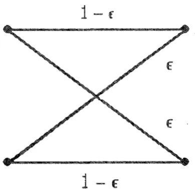
£Figure 2.5. Binary Symmetric Channel
{x1, ... ,xm}· The message is the random variable X with distribution
p(x).
The transmitted message X proceeds through the channel, which stochastically maps to a discrete random variable Y at the channel output. Y takes on one of n symbols from the alphabet Ry ={y1, ... ,
Yn }. The stochastic mapping of the channel is governed by the conditional probability distributionp(ylx)
= P{Y =vlX
=x}.
(2.17)The resulting channel output Y thus has the marginal probability distribution
p(y)
= ~p(x)p(ylx) .
[image:45.514.156.351.112.301.2]33
-As a concrete example of a discrete communication channel, consider the binary symmetric channel (BSC) shown in Fig. 2.5. Here the input and output alphabets
are identical; that is, - Ry =
{0, 1}. \Ve will assume the input probability
distribution is{
P x - O·
p(x)= 1'-p, x=l'. (2.18)
The conditional probability distribution that governs the channel behavior is
{
1 - e, x = 0,y O;
( I
x) =
e, x = 0,y = 1;P y e, x l,y = O;
1 - £, x - l,y = 1.
(2.19)
If we assume that the goal of the BSC is to reproduce faithfully the input symbol
at its output, then it can be seen that the probability of error for the BSC is £,
and the probability of correct transmission is 1 - £. Of course, we would intuitively expect that the smaller £, the better the channel. Let us verify this by calculating
the mutual information between X and Y for the BSC. From Eq.s (2.2) and (2.9) we have
H(X) = -p logp - (1 - p) log(l - p),
and
H(XIY) - -p(l - e) log(l - e) - pdog £
- (1-p)(l - e)log(l - e)- (1-p)eloge
= -dog£ - (1 - e) log(l - e). Thus, from Eq. (2.10) we have (noting that I(X; Y) ~ 0)
---
---~---t---._log 2
0.0 0.5 1.0
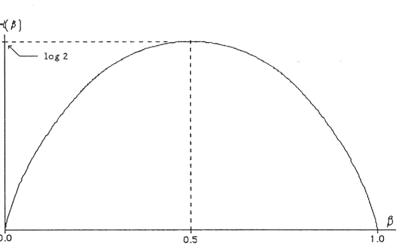
Figure 2.6. The Binary Entropy Function 'H.(/3).
If for all j3 E [O, 1], we define (recalling as above 0 log 0 = 0)
'H.(/3) = -/3 log/3 - (1 - /3) log(l - /3), (2.20)
then
I(X;
Y) =max[ 0, 1-l.(p) -1-l.(i;)], (2.21)where 1-l.(/3) is called the binary entropy function.
[image:47.524.59.458.80.325.2]35
-I(X; )
as given Eq. (2.21), we note that for allp and€ such that 11.(p)>
1i.(E),I(X;Y)
is just the difference 1i.(p) -1i.(E), and for all other p and E, I(X;Y) is zero. From Eq. (2.21) we see thatI(X;
Y) is maximized whenp = 0.5. · can be seen by noting that Eq. (2.21) is maximized when 11.(p) is maximized, and 11.(p) isma.ximized when p = 0.5. So the BSC provides the maximum mutual information between input and output when the input symbols 0 and 1 are equiprobable. \Ve
also see that
I(X;
Y) is maximized when 11.(E)
= 0, which occurs when either€= 0 or € 1. That this is true for € - 0 makes intuitive sense, since this is the case inwhich no errors whatsoever occur. That this is true for the case of € = 1 may at first seem surprising, since this is the case of the channel's always making an error.
But if a binary symmetric channel always makes an error, X = 0 always produces
Y = 1 and X - 1 always produces Y = 0. Such a channel is really a very reliable channel. The receiver simply assumes that when Y - 1 is received, X = 0 was sent, and that when Y = 0 is received, X = 1 was sent.
Of particular interest is the fact that for all p and€ such that 11.(p) ~ 1i.(E),
I ( X; Y) = 0, and the channel is of no use whatsoever. In such cases, the channel error rate € satifies the following inequality:
for all p and € such that 1i.(p) ~ 1i.(€).
Such channels are of no use m conveymg information m effect there is
greater uncertainty in the channel's performance than there is in what message was sent. If one chooses the most likely symbol to be transmitted as the transmitted
rule based on actual observation of the channel output.
the above example, we noted that for any given binary symmetric channel and associated 7-l(E), p = 0.5, the mutual information I(X; Y) was max-imized. general, any channel with mutual information I(X;Y) H(X) -H(XIY), there will be a maximum value of I(X; Y) over all probability distribu-tions p(x ). This quantity is known as the capacity of the channel. We will denote the channel capacity by C. Thus, the channel capacity is defined as
C
= max{I ( X;
Y)}.;:{x) (2.22)
The channel capacity is the largest rate at which information can be transferred
across the channel. Shannon [2.2] showed more importantly not only that the capacity C of a channel was the maximum rate at which information could be sent across the channel, but also that, with proper encoding, information can be sent
across the channel at any rate less than C with arbitrarily small error. The capacity
37
-2 • Theory
c
Variables.In the previous section, we examined entropy and mutual information for discrete
random variables and vectors, but usually, and particularly in this thesis, we are in-terested in the case of continuous random variables and vectors. vVe will now obtain
expressions for the mutual information between two continuous random variables.
Consider a continuous random variable X defined on the real line R with probability density function (PDF) f(x). The differential entropy of X is defined by
00
h(X) = -
j
J(x) log /(x) dx. (2.23) -ooThe differential entropy is not the limit of the Riemann sum obtained. by discretizing
the real line into intervals of size .6.x [2.1]. For such a case we would have a Riemann sum of the form
But
lim
H(X)
=
lim {- Lf(xk)logf(x;;).6.x}~s_,O ~s_,O
k
= lim {- Lf(xk)log/(xk)}+ lim {-log.6.x}
~s_,O ~s-0
k
00
=
-!
f(x)logf(x)dx- lim {log.6.x}.~s_,O - 00
- lim {log .6.x} = oo,
~s-0
(2.24)
Assume we another continuous random variable defined on R and that and Y are jointly distributed with joint PDF f(x,y). Assume also that f(x) is the marginal pdf of
X,
f
(y) is marginal pdf of y,f
(xjy) is the PDF of Xconditioned on , and
f
(y Ix) is the PDF of Y conditioned on X. \Ve can then define the joint differential entropy00 00
h(X, Y) == -
j j
J(x,y)logf(x,y)dxdy, (2.25)- 0 0 - 0 0
and the conditional differential entropies
00 00
h(XjY) == -
j j
f(x,y)logf(xjy) dxdy, (2.26) -oo -ooand
00 00
h(YjX) == -
j j
f(x,y)logf(yjx)dxdy. (2.27) -oo -ooConsider again the limiting process of the Riemann sum approximation to an entropy, but this time using the conditional entropy H(XjY). In the limit as .6.x -+ 0, we obtain
lim lim H(XjY) == lim lim {-L L f ( x1,y1;).6.x.6.yiogf(xJIYk).6.x}
C.s-+O Ay-+0 ..:).s-+O As-+O
j k.
- lim lim {-
LLf(xJ,Yk).6.x.6.ylogp(xJIY.~)
As-+ 0 As-+ 0
j k
- lim lirn {'\:"""' J(x1,yk).6.x.6.yiog.6.x}
As -+ 0 C.s -+ 0 L..;
J k
00 00
- j j
f
(x, y) logf
(xjy) dx dy - lim log .6.x.As-+O
- 0 0 - 0 0
(2.28) Again, we note that the second term of the Riemann sum diverges as .6.x -+ 0, so
39
-term that results the limit is what we have defined as the differential entropy of
conditioned on
considered evaluating the entropy of a continuous random variable by dis-cretizing it into intervals of length l::,.x and forming a Riemann sum representing the
entropy of the discretized random variable, and then letting l::,.x go to zero. This was not useful because the Riemann sums diverge as l::,.x goes to zero. In both
Eqs. (2.28) and (2.29), the problem was a term of the form - log l::,.x. If, however, we do the discretization of both
H(X)
and H(XjY), form the mutual informationI(X;Y), and then take the limit as l::,.x--+ 0, we obtain lim
I(X;
Y)=
lim {H(X) - H(XJY)}Aa:---.O Aa:-+O
-h(X)-
lim log/::,.x-[h(XJY)- lim log!::,.x]Aa:->O Aa:-+O
(2.29)
=
h(X) -
h(XJY) lim [log l::,.x - log !::,.x]Ll.a:-+ 0
=
h(X) -
h(XjY).Thus, in the limit, as l::,.x --+ 0, we have that the mutual information is well defined and is given by
I(X;
Y) =h(X) -
h(XJY). (2.30)So the mutual information between two jointly distributed continuous random vari-ables X and is given by Eq. (2.30). A more detailed proof of this relationship is given in Reference [2.1). The above argument, however, illus~rates the process by which (2.30) is obtained.
The mutual information