Ames Laboratory ISC Technical Reports Ames Laboratory
3-1955
Ratio of solid velocity to mixture velocity in slurry
flow
Richard J. Burian
Iowa State CollegeGlenn Murphy
Iowa State CollegeFollow this and additional works at:http://lib.dr.iastate.edu/ameslab_iscreports Part of thePhysics Commons
This Report is brought to you for free and open access by the Ames Laboratory at Iowa State University Digital Repository. It has been accepted for inclusion in Ames Laboratory ISC Technical Reports by an authorized administrator of Iowa State University Digital Repository. For more information, please [email protected].
Recommended Citation
Burian, Richard J. and Murphy, Glenn, "Ratio of solid velocity to mixture velocity in slurry flow" (1955).Ames Laboratory ISC Technical Reports. 97.
Abstract
The study consisted of two parts, a theoretical analysis of the problem and an experimental investigation under controlled conditions. The theoretical analysis resulted in an equation which expressed the velocity ratio in terms of dimensionless parameters representing the distribution of the particles in the mixture, the slip between the solid particles and the adjacent fluid, and the velocity distribution of the fluid in the conduit.
Keywords Ames Laboratory
Disciplines Physics
:r
5
c.w().ICLASSI FlED
AL
I5c..-5~~
UNCLASSIFIED
/
ISC-586Subject Category: ENGINEERING
COMMISSION
RATIO OF SOLID VELOCITY TO MIXTURE VELOCITY IN SLURRY FLOW
By
Richard J. Burian Glenn Murphy
March 1955
Ames Laboratory Ames, Iowa
This report was prepared as a scientific account of Govern-ment-sponsored work and is made available without review or examination by the Government. Neither the United States, nor the Commission, nor any person acting on behalf of the Commis-sion makes any warranty or representation, express or implied, with respect to the accuracy, completeness, or usefulness of the information contained in this report, or that the use of any infor-mation, apparatus, method, or process disclosed in this report may not infringe privately owned rights. The Commission assumes no I iabi I ity with respect to the use of, or For damages resulting with respect to the use of any information, apparatus, method, or proc-ess disclosed in this report.
This report has been reproduced directly from the best available copy.
Printed in USA, Price
50
cents. Available from the Office of Technical Services, Department of Commerce,I.
II. III.ISC-586 TABLE OF CONTENTS ABSTRACT
INTRODUCTION
REVIEW OF LITERATURE HATERIALS AND EQUIPMENT
A. Haterials
1. Size determination
2. Specific weight determination
B. Equipment
IV. EXPERH'JENT AL PROCEDURE
A. Velocity Ratio Tests B. Solid Distribution Tests
V. THEORETICAL APPROACH VI. EXPERIMENTAL APPROACH VII. DISUCSSION
VIII. CONCLUSIONS
IX. SUGGESTED TOPICS FOR FURTHER INVESTIGATION X. SUGGESTED CHANGES IN THE EQUIPMENT
XI. SUMMARY
XII. LITERATURE CITED XIII. APPENDIX
A.
Derivations of Equations Used1. Determination of concentration
2. Determination of velocity ratios
B. Experimental Data
1. Velocity ratio tests
2. Solid dlstribution tests
Ames Laboratory at
Iowa State College F. H. Spedding, Director Contract No.
W-7405
eng - 82RATIO OF SOLID VEIDCITY TO MIXTURE
VELOCITY IN SLURRY FLOwl
by
Richard
J.
Burian and Glenn MurphyABSTRACT
The study consisted of two parts, a theoretical analysis of the problem and an experimental investigation under controlled conditions. The theoretical analysis resulted in an equation which expressed the velocity ratio in terms of dimensionless parameters representing the distribution of the particles in the mixture, the slip between the solid particles and the adjacent fluid, and the velocity distribution of the fluid in the conduit.
In the exoerimental part of the study a dimensional analysis was performed on the variables which seemed most likely to influence the problem. The dimensionless parameters were then combined into a single equation by use of the principles of similitude. In this way the equation obtained is entirel;}r general within the range tested. The tests were performed on slurries composed of several types of glass, steel and lead spheres in water flowing through a glass tube. The conclusi~ns drawn include: the velocity ratio (l) increases as the size of the particles and the velocity increases, (2) decreases as the density of the particles increases, and (3) is independent of temperature and concentration.
The equation obtained from the theoretical analysis was written in the form of the experimental equation and the corresponding terms compared. Since the theoretical analysis involved several simplifying assumptions, it was thought that one or several of these caused some di,screpancy in 1 the results. The various assumptions were discussed and the ones most
likely in error pointed out.
ISC-.586 1
I. INTIDDUCTION
The use of slurries, or fluidized solids as they are sometimes called, is becoming popular for certain types of materials handling operations. Slurries can be used to advantage for moving bulk materials as grain, coal,
ash, sand, gravel, cement and powdered chemicals. For thesetypes of
materials slurries provide a clean, low cost and easy method of transport.
In its broadest sense, a slurry may be defined as a suspension of solids in a fluid. Some fields of engineering limit this definition to include only stable suspensions {suspensions in which the particles will not settle out such as thick mud, paste, etc.), suspensions using only a specific fluid or suspensions containing particles within a certain size range. Other fields such as those concerned with wind and sand erosion make use of the definition in its broadest sense.
The engineer designing a slurry system for materials handling must consider such factors as power consumption, efficiency and mass rate of flow of the solid. However, he must also consider erosion of the conduit and the effect on the shape of the particles due to the jostling they receive during transport and stopping at their destination. It would
therefore be advantageous for him to be able to predict the average velocity of the particles in the flow of a slurry. Little is yet known, however, about the physical laws which govern slurries and in the past the engineer has had to rely almost entirely upon trial and error in the design of slurry systems.
The investigation was performed with the intention of adding to the knowledge of the physical characteristics of slurries. The specific object was to develop an expression for the ratio of the average velocity of the solid component to the average velocity of the entire mixture in a slurry. The problem was approached from both the analytical and experimental view-points and the results compared.
II. REVIEW OF LITERATURE
A search of the literature revealed that little work was done on studying the laws governing slurry flow before about 193.5. All the work done before this time and a good share of that done more recently has concerned itself with specific cases and as a result little is known today about the general behavior of slurries. Some investigators have, however, made generalizations from the results of their studies.
most of the sand was dragged along the bottom of the pipe at a low velocity and the other in which all of the sand vias suspended in the fluid and
flowing rapidly. In between these two regions existed a transition reeion where part of the sand was dragged along and part of it was suspended. The
upper limit of the low velocity region was determined to be from
3.5
to 4fps while the lower limit of the high velocity region was determined to be
from 4 to 10 fps depending upon the coarseness of the sand and the uniformity of size.
Howard (17) observed the same type of flow regions in tests with sand
and water in a 4-inch, horizontal pipe. However, he noticed that in the
transition region the layer would move spasmodically. He defined the upper
limit of the low velocity region to be abolt 6 fps and the lower limit of
the high velocity region to be about
7.5
fps.In this same series of tests, Howard (16, 17) also determined the
distribution of the solid in the mixture. He used a 7/16-inch diameter sampling tube which he could place at any point on the cross section of the
pipe. From his tests on plain walled pipe he obtained a series of diagrams
of the cross section of the pipe with contour lines representing the
per-centage of the total solid flowing above the contour. The contour lines
were approximately parallel to the horizontal diameter of the cross section indicating that the di~tribution of the solid varies only with the vertical distance from the center of the pipe and not with the radial distance.
From his tests Howard concluded that the majority of the solid flows in the
lower third of the pipe. Tests of this same nature were conducted by
Gladfelter (13) on pipes containing rifling. The rifling actually consisted of helical vanes on the inside of the pipe. From his tests, Gladfelter
found that the rifling caused a more uniform distribution of the solid.
Richardson (23) defined three similar regions of flow for open
channels with the exception that all three regions could exist simultaneously,
within the channel bed, at the boundary and in the main stream.
As a result of his studies on pneumatic handling systems, Korn (19) defined three modes of particle transport. In the first of these the velocity is so low that the particle skips or hops alo~g the bottom of the
pipe with the length of each jump dependent upon the momentum of the particle.
As the velocity is increased, the velocity gradient of the fluid becomes so
steep near the pipe wall that the difference in pres~:ure across the diameter
of the particle causes it to be drawn toward the center of the pipe and the particle strikes the pipe wall only occasionally. In the third mode of
transport the particles are so fine that the entire mixture acts as a true
fluid. The first of these modes of transport can be said to be sb:ilor to
the transition region of flow as defined by Blatch and Howard while the
second mode is similar to the high velocity region. The third mode of
ISC-586
3
The velocity at which the particles settle out faster than they are picked up into suspension was defined by Wood and Bailey (28) as the choking velocity. They concluded that it is approximately the same for all concen-trations. Chatley (5) stated that since other experimenters have found the components of the velocity of the fluid particles perpendicular to the direction of flow at full stream turbulence to be about 15% of the mean flow velocity, the particles of solid should be suspended when the mean velocity of the fluid reaches a value 6 to 7 times the settling velocity for the particles.
The mechanism of particle transport was studied by White (25). He stated that at low velocities the drag on the particles by the fluid is almost entirely a function of the viscosity of the fluid while at high velocities the drag is primarily due to the pressure drop across the "length" of the particle.
Dobbins (12) stated that the mechanism causing suspension in turbulent flow operates on the law that two masses can not occupy the same space at
the same time. When an incremental volume of mixture in the stream flows upward due to turbulence, an incremental volume of mixture at some other point in the stream must move downward. If the concentration of the solid is greater at the lower levels, the incremental volume moving upward goes from a region of high concentration to one of low concentration while the incremental volume moving downward goes from a region of low concentration
to one of hir,h concentration. The net effect is an upward transport of solid. ~fter a time the net upward transport will be balanced by downward transport due to gravity. Dobbins assumed equilibrium to exist and arrived at the expression
where Vl is the settling velocity, ~ is an exchange coefficient between the two levels, Yl and Y2 are the distances from the stream bottom to the two levels and C1 and C2 are the concentrations at these two levels. Wood and Bailey (28) derived an equation for the flow of particles in a gaseous medium. The equation was of the form
where x is the distance traveled (in feet) by the particle from rest, v
the roughness of the conduit wall. This equation indicates that the particle must travel an infinite distance before it attains its maximum velocity. This is because a state of equilibrium can not exist since the gas is continually expanding as it flows through the conduit and the particles continue to be accelerated in the directioP of flow.
The most thorough analysis of the forces acting on a particle in a compressible fluid was per.f'ormed by Pinkus (21). The first part of his analysis, taken from DallaValla {10, pp 24-29), was for the motion of a particle in a two dimensional field. Newton's Second Law of MOtion was applied in the directions of the two axes and an equation in differential form was obtained for the velocity of the solid. This equation contains a drag coefficient which can be assumed to rg11ow either of two different patterns.
Pinkus first assumed that the coefficient was a constant and integrat~d the equation. For this he obtained Vs ~ 1
v f
,1-~~
.
I'Fw'i'tj=o=cA===
where vs is the ratio of the velocity of the solid to the velocity of Vf
--the fluid, f is the-Fanning friction factor, m is the mass-of' a particle, D is the pipe diameter, ~ is the density of the fluid, C is the drag
coefficient and A is the projected area of the particle.
4.8
In the second case, Pinkus as~umed that y!C:= 0.63 ~ where d is the diameter of the particle and~ is the viscosity of the fluid and v::;: {vrvs)• Upon integration the equation became Vs ~ 5 ..
A
~-1 ~
• .L
""'"l't2V=-r~Pr-where
L23 •
6.o5 ;o.
75vr] -
~r,
S=
-
Ati, L1 ::;:js2
- 4Pr,
2nr
T=
2hr.,2,
andP= 2f - 0.2faA
•
ISC-586
5
Pinkus then performed a series of tests on two siz.es of sand in air. The large sand had a mesh range of 28 to 48 while the small sand had a mesh range of 60 to 100. For the case where the drag coefficient was a constant equal to 0.44 he obtained values of velocity ratio of
0.33
for the small sand and 0.20 for the large sand. When he let the drag coefficient equal the function of Reynolds Number given above, he obtained values of 0.5 -0.6 for the small sand and 0.28 -0.33
for the large sand. He checked these values against published values of velocity ratio calculated from experi-ments b,y Cramp (7) and by Hariu and Molstad (15). Cramp used grain withair as the medium flowing in a horizontal pipe. He determined the velocity of the solid by allowing the grain to discharge into the atmsophere and measuring the distance the grain traveled before striking the ground. Hariu and Molstad performed tests on two sizes of sand in two vertical tubes of 1/4-and 1/2-inch diameter. Their large size of sand was about five times as large as that used by Pinkus and the small size was about two and a half times as large as that tested by Pinbts. Their method of determining the velocity of the solid was developed by Cramp and Priestley (8) and is explained below. Cramp obtained values of velocity ratio between 0.4 and 0.47. Hariu and Molstad arrived at values for the large sand of 0.25 to 0.28 and for the small sand of 0.66 to 0.74.
B.y comparing these values with his own results, Pinkus concluded that the assumption that the drag coefficient is a function of Reynolds
Number is more nearly correct.
Cramp (6) also derived an analytical in vertical flow. It was of the form vs
Vf
equation for the velocity ratio
=
l-
-
~
rw-
where W is thevf
-y ;(
weight of one particle and ~is a coefficient determined
qy
adjusting theupward flow of fluid in the tube until the solids are just suspended but neither rise nor fall. He compared this equation with values obtained experimentally by usinc the method developed by Cramp and Priestley (8). In his tests the velocity of the fluid was varied between 10 and 20 fps.
The analytical and the experimental values differed by about 40% at the
lower end of the range to about 5% at the upper end.
The method used by Cramp and Priestley (8) to measure the velocity
of the solid was to let the slurry flow through a conduit which had two
shutters in it a known distance apart. When the system had been run long
enough to enable them to calculate the weight rate of flow, the shutters
were simultaneously closed, trapping the grain between them. The section
of conduit between the shutters was removed and the weight of trapped solids measured. They were then able to calculate the velocity of the solids from the equation v : ML where M is the weight rate of flow of the solid, L is
s ~
Two other experimenters, Belden and Kassel
(3),
developed an empirical expression for the velocity of the solid in vertical flow in the turbulent region. Their equation was of the formVs ::; 1/2 [v - vi .. Gs ..
j{~
--
=-v
-
1
-
.
-.. - -G-s- ) 2-
-=
-
-4;s viws ws Ws
where vi == 1.32 vkd
(~~
-
-
~
wf) ( l ) and where v is the nominal gas• uJf
velocity, Gs is the weight rate of flow of the solid per unit area, ws is the specific weight of the solid, vi is the "slip" velocity,
g is the acceleration of gravity, d is the particle diameter and wf
is the specific '\-Ieight of the fluid.
Two 11rule of the thumb" equations were developed by DallaValla (ll)
for flow in horizontal and vertical conduits using air as the medium.
For horizontal flow he obtained 'h = 16,200
r
t
s
;&tl
0.4
whilefor ve-t:Lcal flow he obtained vv = 54,700 [ (
~
.. 1 _,:
s1- d •6 where (:..8 is s-the specific gravity of -the particles and d is -the diameter of -the
particles in feet. These equations are for air having a specific weight of 0.075 pcf.
Jones and Hermges ( 18) measured the velocity of the solid in a
transparent tube by taking pictures of the flow. By taking double
exposures, separated by a very short but known time interval, they were able to measure the velocity at which the particles were traveling. Tests
were performed on a mixture of coal in water but the results were not
published.
III. MATERIALS AND ~UIPMENT
A. Materials
In selecting the solids to use for the tests the following qualifi-cations were considered:
1. The solids should be of several different sizes but each size
should be uniform.
ISC-586
3.
The solids should be of several specific weights.4.
The particles of solid should be large enough and dense enough to settle out of water in a short time.There were readily available five sizes of particles which fulfilled
the requirements reasonably well. They consisted of two sizes of glass,
two sizes of steel and one size of lead spheres. Although the larger size glass particles were not perfect spheres but rather more on the order of ellipsoids, it was assumed that this variation would have a negligible effect.
The glass particles were purchased from the Minnesota Mining and
Manufacturing Company, the steel particles from Pittsburg Crushed Steel
Company and the lead from the National Lead Company.
1. Size determination
Two methods were used to determine the size of the particles. One 7
was to take measurements of the particles through a microscope with a
traveling eyepiece. The other was to take magnified pictures of the particles and make measurements of the photographs. By the second method the shape of the particles could be studied more easily.
Samples of the particles were obtained by successive quartering of the
entire amount. The particles were mounted by dispersing them in Canada
balsam between two glass specimen slides.
The magnification of the photographs was determined by preparing slides of small wires of known size and photographing them at the srune time as the particles and with the same camera focusing. The size of the wire used was determined by means of measurements taken under a microscope and checked with a micrometer.
The measurements taken on the photographs were made across two perpen-dicular diameters of each particle. In the case where the particles were oblong rather than spherical, the measurements were made across the major
and minor diameters. The measurements taken under the microscope were made
only in the direction of motion of the eyepiece regardless of the orientation of the particle. The average size of the particles was determined as the arithmetic average of all the measurements.
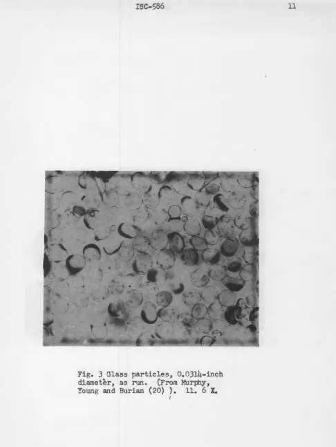
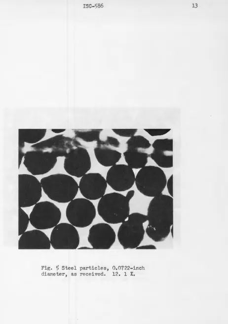
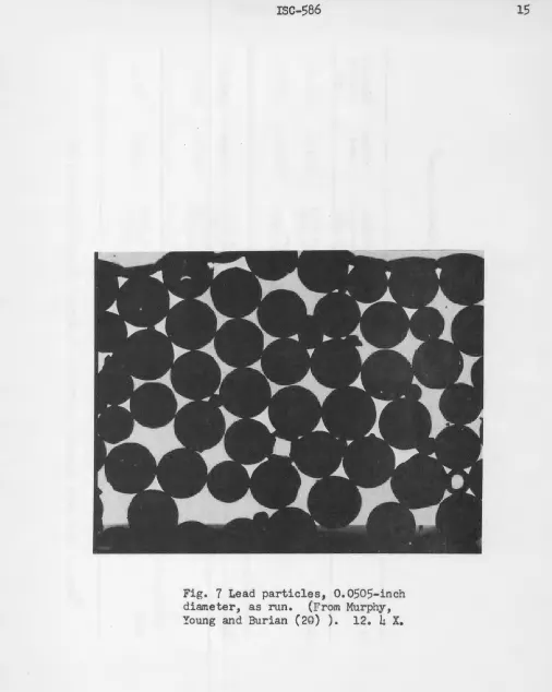
As a check against the amount of breakace or deformation of the particles during the tests, photographs were also taken at the completion of the tests and the results compared to those taken before. It was found that even with the glass, there was no significant difference in the size
of the pictures taken. Those labeled "as received11 are pictures taken before
the tests were performed while those labeled 11as run" are pictures taken after
the tests were completed. In Table l the results of the size determination are tabulated. All but one of the photographs in Figs. l through
7
and most of the data in Table l originally appeared in Murphy, Young and Burian (20).2. Specific weight determination
The specific weight of each size of particles was determineq Qy the method of displaced volume. A representative sample of the particles was
thoroughly dried and added to a graduated cylinder partly filled with a
fluid. The change in the volume readinG and in the gross weight of the
cylinder enabled the calculation of the specific weight of the particles. Two fluids were used in these determinations, water and carbon tetrachloride. The results are also tabulated in Table 1.
B. Equipment
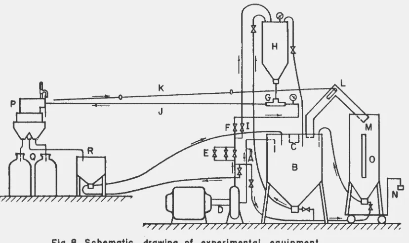
The equipment used in this investigation was used for other studies of slurry flow and was modified for these tests. It cousisted of a pump and motor unit, a water supply tank, a solids feeding tank, a weighing tank, platform scales and a glass test section, pa~t of which could be removed. The glass section was about 12 feet long with an inclined return section of approximately the same length. The inclined section had a slope of about
l inch per foot. The removable piece, which was situated on the incline, was about 47 l/4 inches long and had an internal diameter of approximately 0.3 inches. The exact internal diameter of the removable section varied from time to time because of the breakage experienced with these sections while continuously handling them. The same size tube was used for all the tests on any one size of particle, however. The sizes of the removable sections are included in Table 2 which is in the chapter, Experimental
Approach. The tests to determine the solid distribution were conducted in a horizontal tube having an internal diameter of 0. 314 inches. A schematic
diagram of the equipment is shown in Fig.
8.
Water from an outside source entered the system on the inlet side (A)
ISC-586
Fig. 1 Glass particles, 0.0114-inch diameter, as run. (From Murphy, Young and Burian (20) ). 86. 0 X.
Fig. 2 Glass particles, 0.0314-inch
diameter, as received. (From Murphy,
ISC-586
Fig. 3 Glass particles, 0.0314-inch diameter, as run. (From Murphy, Young and Burian (20) }. 11.
6
X. [image:17.548.30.516.24.670.2]ISC-586
Fig.
S
Steel particles, 0.0722-inch diameter, as received. 12. l X. [image:19.548.60.522.28.684.2]ISC-586
Fig.
7
Lead particles, 0.0505-inchdiameter, as run. (From Murphy,
[image:21.549.11.517.37.671.2]Material
Glass
Steel
Lead
*
Table l
Smnm3.ry of particle size and specific weight ieterminations*
Method of sj ze
determination
microscope photographs microscope photofraphs
microscope photorraphs microscope photographs mic:roscooe photographs
Number of observations
35
80
--161
37
28
40
87
53
117
Maximum observed inches0.0134
0.0136
--0.0474
0.0199
0.0175
0.0812
0.0929
0.0523
0.0598
Minimum observed incheso.oo6o
o.
0091--o. 0215
0.0103
0.0100
o.o612
o.o6Jo
0.0395
0.0373
Average inches0.0114
0.0314
0.0149
0.0722
o.osos
Much of thj~ data appeared ori~inally in Murphy, Young and Burian
(20).
Specific weight
ISC-586
17
[image:23.550.64.478.196.442.2]the water in the inlet line of the pump, fresh water only was supplied to the pump. If at hi~h rates of flow the outside source could not supply the entire amount of water required by the pump, the amount of water that was drawn from the supply tank was so small that no trouble was encountered with the valves plugging. The water in the system was continuously changed by means of the discharge throurh the weir in order to keep the w~ter at a nearly constant temperature. Any fines that were washed out the weir were collected and periodically added to the system.
The pump and motor unit (D) consisted of a l-inch Worthington Slurry Pump driven by a 5-hp electric motor. Since the pump was a slurry pump no difficulty resulted from allowing the fines to pass through it. With this unit velocities up to 22 fps were obtained.
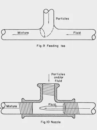
The rate of flow through the glass section was controlled by a bank of three valves (E) in parallel. The valves were of different sizes to enable coarse and fine adjustments of the flow. A quick-closing valve (F) was used to stop the fluid flow sharply. The solids were fed into the glass section by the feeding tee (G) from the solids feedinr, tank (H). A sketch of the feeding tee used is shown in Fig.
9.
The rate of solids feeding was con-trolled by regulating the pressure in the feeding tank with the valve (1).For the tests to determine the velocity ratio of the solid to the mixture, the mixture flowed from the feeding tee through the horizontal part of the glass section (J) and back through the inclined part. On the incline between the bend and the removable section (K) was a "settling" section about 60 diameters long. When the mix~ure reached the top of the inclined section it was directed by the ~flipperfl (L) into either the supply tank or the weir,hing tank (M).
The weighing tank, resting on platform scales
(N),
had a glass window (0) in the side upon which was a piezometer scale for obtaining the volume of mixture in the tank. In the bottom of the weighing tank was a 3/4-inch pipe tee into which was constructed a nozzle for "sucking" the particles and the fluid from the tank and forcing them to flow back into the supply tank. A sketch of the nozzle is shown in Fig. 10. A similar nozzle was situated at the bottom of the supply tank for moving the particles up to the feeding tank.For the tests to determine the solid distribution the inclined section of the glass tube was cut out of the system and a separator (P) placed at the end of the horizontal section. From the separator the mixture flowed either into the two carboys (Q) or into the waste bucket (R). In the bottom of the waste bucket a nozzle similar to the one in the bottom of the
Mixture
ISC-586
Particles
Fig. 9 Feeding tee
1
Particles and/or fluidFig.IO Nozzle
19
[image:25.547.92.433.106.563.2]The separator, shown in Figs. 11 and 12, ~onsisted of three components, the flow divider, the ttflipper" and the multiple fnnnels. The flow divider consisted of a metal plate which attached to the frame supportinf, the glass conduit, and a slidinr~ box. The box was divided into two compartments as shown in Fir. 12 with the front of the dividing wall filed to a knife edge. A micrometer which had the anvil removed by cutting the C-section at about
the center was attached to the metal plate by the stub end of the C-section. The spindle of the micrometer was attached to the top of the sliding box by means of a flat brass beadng. Four sprinp:s were attached from the metal plate to the back of the sliding box to hold it a~ainst the plate and to support its weight. Hith this arrangement it was possible to move the knife edrc;e vertically across the end of the r·lass tube and cut the flow at any desired distance from the bottom of the tube.
The flipper was located directly below the divider. It consisted of two funnels attached to each other and mounted upon bearings in such a way that the flow from the divider could be directed into either side of the multiple funnel unit situated below. The multiple funnel component was divided into three sections. One section extended across the entire back of the unit while the other two comprised the front half. The back funnel discharged into a tube leading to the waste bucket while the front sections discharged into tubes leading to the carboys. The carboys, each of which had a capacity of five gallons, had piezometer scales on the side to measure the volume of the mixture collected in them.
Additional pieces of equipment included a mercury thermometer, a triple beam balance, a Toledo scales, a stop watch and a 3/8-inch pneumatic vibrator to aid in controlling the solids feeding rate. For a time, an Erector Set motor with a bad set of bearings was used as a vibrator before the pneumatic one was obtained. \<!he rever possible, flexible tubing was used in preference to pipe or metallic tubing. For areas where the pressure did not exceed 35 psip;, tygon tubing was used. Although it would stand hip,her pressures at temperatures in the neirhborhood of 20° C, it would swell to the burstinr;
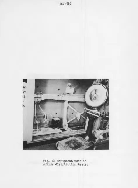
point when tests at 50° C were being conducted. Therefore, in the parts of the system using flexible tubing and where the pressure exceeded 35 psig, cloth reinforced rubber tubing was used. Pictures of the equipment are shown in Figs. 13 and 14.
IV. EXPERIME~!TAL PROCEDTTRE
ISC-586
Fi~. l l Close-up view of
the separator equipment.
/
,..,
/
/
/
23
ISC-586
25
A. Velocity Ratio Tests
The steps used for collectinr the data for the solid to mixture velocity ratio are given in the following outline in sequence.
1. The tap water was turned on and adjusted to the desired temperature.
2. The solids were forced by the nozzle at the bottom of the supply tank from the supply tank up to the solids feedinr. tank and the tank bled of any air. It was thought necessary to bleed the feed-ing tank to provide a const~nt head of water above the particles and thus avoid a possible source of trouble. It was noticed on occasion that when an excessive amount of air was present the rate of feeding of the solids became difficult to control.
3.
After the weighing tank was checked to be sure that it was empty and the scales upon which it rested were balanced, the motor driving the pump was started.4.
Fluid alone was allowed to flow through the test section and dis-charge back into the supply tan,k. The gage pressure immediately upstream of the feeding tee was increased to the necessary value to obtain approximately the desired velocity.5. The clamp on the tygon feeding tube was released and the pressure
in the feedin~ tank was increased until the feeding rate of the solids was such that the desired concentration was obtained. At low velocities it was possible to check the concentration before running the tests by collecting the slurry in a 500-ml graduated
cylinder and measuring the net weight and volume from which the specific weight could be calculated. The value of concentration could then be read from a ?raph of concentration versus specific weight. At high velocities it became impractical to use this method because of the rapidity with which the cylinder was filled. However, i f the tests for any one concentration were ~n starting with low velocities and proceedlng by increments to the higher velocities, when it became impractical to check the concentration each time, it was possible to see the trend in the concentration
change and to make the valve adjustments accordingly. In this way the desired concentration could usually be obtained within 1 to 2%.
6~ When equilibrium had been reached the test was begun by directing the flow into the weighing tank and starting the stop watch
simultaneously.
8.
After checking to be sure that the system was still in a state of equilibrium, the quick-closing valve and the tygon feeding tube were sharply closed and the pump motor turned off.9.
The weighing tank scales and the piezometer readings, the time and the temperature were recorded.10. The fluid was allowed to drain slowly out of the inclined section and the removable tPst section removed in such a manner that none of the particles lying on the bottom of the tube was lost. One end was stopped with a cork and water taken from the supply tank was poured in the other. The water was taken from the supply tank to obtain, as nearly as
possible, water of the same temperature as that with which
the test was run. The other end of the tube was then stoppered, the tube weighed on a triple beam balance and the length between the corks measured.
11. After all of the data vrere recorded, the rrixture in the weighing tank was pumped to the supply tank. When the quantity of part-icles collected in the supply tank became so great that it was thought an insufficient amount was left in the feeding tank to allow another run, the p-artictes were again moved up to the feeding tank.
Tests were run over a range of velocities for three different concentration ranges and at three different temperatures. The limits for each concentration range were considered as !
2.5%.
The nominal concentrations were generally 10, 20, and30%.
H9wever, for the tests on lead, 40% was substituted for the 10% since because of the density of the lead, a small number of particles was left in the test section when the system was stopped. This resulted in a large percentage error for a small error in the weight of the tube and mixture. The temperatures at which the tests were run were approximately 17,35
and50°C
although for the smaller size of glass particles, a series of tests were also run at about8°C.
The temperatures were controlled by proper adjustment of the hot and cold water taps except the latter which was obtained by adding ice to the supply tank and turning off the water taps entirely. The temperatures tended to be greater at low velocities than at high velocities. It is believed that this was due to the increased"churning" in the pump at the low rates of flow.
Some difficulty was had with the control of the feeding rate of the solids for the larger steel particles. This was overcome by increasing the size of the feeding tee and attaching a vibrator to the tee. At first the only thing available for a vibrator was a small Erector Set motor with a worn set of bearings. This provided ample vibration to allow good feeding control. Later a pneumatic vibrator was purchased to
Isc-S86 27
B. Solid Distribution Tests
The procedure used to conduct the tests for determining the solid distribution was quite similar to that just given. Steps 1. through 6. were identical with the exceptions that in step
J.
the separator micrometer was adjusted to the desired reading and the tare weight of the carboys was taken instead of balancing the weighing tank scales, in step4.
the slurry was directed into the waste bucket before the test was ber,un rather than back into the supply tank, and in step 6. when equilibrium was reached the flow was directed into the carboys. From this point the procedure differed somewhat.7. When either of the carboys became full the flow was directed back into the waste bucket and the stop watch stopped.
8. The feeding tube was clamped off and the pump motor stopped.
9.
The piezometer readings of the two carboys, the rross weight of each of the carboys, the time and the temperature were recorded.10. The carboys were emptied into the waste bucket and the particles transported back to the supply tank.
Tests were conducted at three velocities of approximately 7.5, 15.0 and 21.1 fps and at combinations of five concentrations of approximately 10, 15, 20, 2S,and 30% on the smaller size of p,lass particles. At each concentration £or each velocity nine runs were made with the separator micrometer set at a different position each time. In this way nine points were obtained for the curve of percentage of the solid above h versus
B-where h is the distance from the bottom of the tube to the knife edge and Dis the diameter of the tube. For each group of nine runs the velocity and the concentration were held as nearly constant as possible. All tests were run at tap water temperature which varied between 12.7 and l5.8°C.
For both types of tests sufficient calculations were made after each run to be sure that no gross error was made in any of the readings. The data for the tests are tabulated in the Appendix.
V. THEORETICAL APPROACH
In order to obtain an analytical expression for the ratio of the velocity of the solid to the velocity of the mixture in the flow of a slurry, several assumptions were made. It was first assumed that the
mixture flows at a constant veloci~ and that the distribution of the solid particles in the tube does not change with respect to length or time. It was further assumed that the distribution of the particles is only a
function of the vertical distance and not of the distance from the center of the tube. This last assumption is based on results of experiments performed
distribution of the fluid analytically an equation was assumed. '!he equation for the velocity of the fluid was taken as
vr
=
vo
(R - r)n (1)R
where v is the velocity of the fluid at a distance r from the center of
r
the tube, v is the velocity at the center of the tube, R is the radius of the tube
an8
n is an unknown which is constant for any given velocity of the mixture. It was also assumed that the presence of the particles does not affect the shape of the velocity curve.The slip was defined as
v - v
S - r p
vr
where vp is the velocity of the particle at r.
vp := vr (1 - S).
(2)
Then
(2a)
It was assumed that at any given mixture velocity the slip is a constant. The average velocity of the total solids passing through the tube is
where N. is the number of particles passing through an incremental area
per unit time and the summation is over the cross section of the tube. This can be rewritten as
where
(3)
(3a)
or
ISC-586
dN ~ e.Lda l.
29
V t (4a)
p
where d~ is a differential volume rate of flow of mixture, ei is the volume concentration of particles in the mixture passing through the differental area (defined as the volume of the particles per volume of mixture per unit area), V is the volume of a single particle, L is an arbitrary length, t is th~ time and da is the differential area. From
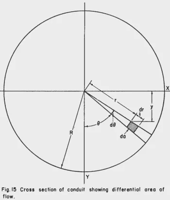
Fig. 15 it is seen that da
=
r dr dg. (5)If equations (1), (2a), (4a) and
(5)
are substituted in equation (Ja) there resultsei r dr de
(6)
This equation could not be integrated, however, until an expression for ei was obtained. Rather than to assume an equation it was decided to run a series of tests and from them to arrive at a logical form for the equation. The method in which these tests were performed was explained in the chapter, Experimental Procedure.
In these tests the slurry flow was divided into two parts by a hori-zontal knife edge placed alternately at different heights in the stream. The percentage of the solid flowing above the knife edge was then calculated and plotted versus~ as shown in Figs. 16, 17, and 18 where h is the vertical distance from the bottom of the tube to the knife edge and D is the diameter of the tube. This method assumes that the solid distribution is only a function of the vertical dimension as indicated by Howard (16, 17).
Figs. 16, 17 and 18 were plotted from tests conducted at three mean mixture velocities and for combinations of five different weight concen-tractions. These figures were then used to determine the relative solid distribution curves shown in Fig. 19. These were obtained by dividing the
~ean curves drawn in Figs. 16, 17 and 18 into ten equal increments in the _ direction, detenn:lming the percentage of the solid flowinv, through the
y
Fig. 15 Crou section of conduit showing differential area of flow.
[image:36.544.94.444.133.543.2]ISC-586
31
1.0 I I I I I -1.0
r-
-g
=0.0363&.
2.85-~
SymbolPt
_!!.__-•
10•1.-~\
0 20•1.+
30•1.-1-
\
-0.9
0.8
0.7
-0.8
-0.6
-0.4
1-1\
-'
0.6 -0.2
0.0-k
1-"'
-t-
."'
-l'\.
t-
\
-0.4
0.3
0.2
0.4
~!'to
1--
\-
1--l\
I I I I
0.2
0.1
0.0 1.0
0.6
0.8
0 20 40 60 80 100
1.0 -r.o
0.9
%=0.0363 -0.8
Symbol es 0.8
•
m.., •
-0.60
oo•t.
+
30~.0.7 -0.4
0.0 1.0
0 20 40 100
ISC-586 33
1.0 -1.0
0.9
~
= 0.0363 -0.8Symbol es
0.8 -0.6
•
15%0 25%
0.7 -0.4
0.0 1.0
0 20 40 60 80 100
Percentage of solid above h
-1.0 r--~-.,..--,...-.,..--,...-,..---,---r---r--r--.-.----r-.---,r---r--r---r-__,
-0.8
-0.6
-0.4r---~----~----~----+-~~+---~~~;---r---r_,
-0.2 y
R
o.o0.2
0.4
0.6
0.8
. __ Symbol
•
0
+
Vm es
7.5 f p s 10,20,30% 15.0 fp s 10,20,30%
21.1 fps 1!5,2!5 01.
1.0, _____ ~~-~~-~~-~~-~~-~~-~~-~---~~~
0.0 0.2 0.6 0.8 1.0 1.2 1.8
Relative solid concentration-3
ISC-586 35
area of the tube cut off in this increment, and dividinG this by the
fractional area through which it flows. The values obtained were assumed
to be the values existing at the center of each increment and were plotted
av,ainst
!,
where y is the vertical distance to the center of the incrementfrom theRhorizontal center line of the tube cross section and
R
is the radiusof the tube. The relation between~ and! can be seen in Figs. 16, 17, and
18 where the two are shown as ordinRtes onRapposite sides of the graph.
It was assumed that the curves in Fir,. 19 could be approximated by a
polynominal equation of the third degree. The equations so obtained for the
different velocities are
7.5 fps:S"
~1.46 r~l.l9 (~)- 0.752(~)
2
-l.36(ft)J_J,15.0 fps:
b'
= 1.66 [1+0.053(~)
- l.03(ft) 2 +0.057C'j)j '21.1 fps:
S
=
1.44~-0.070 (~-
0.477(~)
2
+0.165(i)~.
(7)
(8)
(9)
Since the relative solid concentration,
5
,
represents the incrementalvolume concentration at any point in the tube, the equation can be thought
of as exoressi.ng the distribution of the solid in the tube. Then in equations
(7), (8) and
(9),
e. would replace~ , the concentration per unit area at the center of the tUbe, e , would replace the multiplier on the right sideof each equation, but the0constants inside the brackets would remain the
same for each equation since they determine only the shape of the curve.
IImvever, for the purpose of using this form of equation for the concentration
distribution term in the derivation of the equation for the velocity of the
solid, the constants inside the brackets were replaced by a, b and c to
make the equation general. In the general case, the concentration at any
point in the cross section of the tube is
ei
= •
0~.aCftl
+b(~)
2
+ c(~)
3
~
•
(10)
From Fig. 15 it is seen, however, that
y
=
r cose
• (ll)If eq11ations (10) and (11) are substituted in equation (6) the expression
+c{~cose~
r dr degives
This equation when integrated
= 8(1-S)v0
vs
cn+l) l (n+2) + -( - - ) n+l -(--)-(--)-(n+2 3b n+3 ·-n+-4) • ( 13 )
~
The term, v , can be eliminated by replacing it with an expression
involving the me~n velocity of the fluid. I f the assumed equation for the
velocity distribution is integrated over the entire cross section of the
tube one is able to obtain an equation relating the mean veloci~ of the
fluid to the veloci~ at the center of the tube. Then
. (Avr da
v ::::) 0 .
f
loA
dawhere vf is the mean velocity of the fluid. Substituting equations (1)
and (5) in equation (14) and integrating gives
1
(n+l) (n+2) •
Dividing equation (13) by equation (15) gives
vs
=
4(1-S)Vf 4+b
(i
l
---=-3b_l.
L
(n+3) (n+4):J
(14)
(15)
(16)
The ratio of the mean velocity of the fluid to the mean veloci~ of
the mixture (derived in the Appendi~ is given by
Vf
=
f
S -em
ISC-586
31where
fs
is the density of the particles, em is the density of the totalquantity of mixture transported and {mt is the density of the mixture in
a given length of tube. The difference between the two mixture densities is discussed in the Appendix.
Multiplying equation (16) by equation (17~ gives
4(1-S)
4+b
ri
+ 3b / .
L-
(n+3) (n+4'.J(18)
This is an expression for the ratio of the veloci~ of the solid to the veloci~ of the mixture in terms of three unknowns; n, which controls the fluid velocity distribution; b, which controls the solid distribution; and
S, which is the slip between the fluid and the particles.
VI.
EXPERIMENTAL APPROACHThe experimental approach was begun
qy
first performing a dimensional analysis. The following list of variables was considered as possibly having an influence upon the ratio of the velocity of the solid to the velocity of the mixture:symbol dimensions
g ~
ML-3
ML-lT-1
MT-2
L
L
ML-3
ML-3
LT-2
mean velocity of the solid mean veloci~ of the mixture
density of the fluid
viscosity of the fluid
surface tension
Diameter of the tube
diameter of a particle
density of the particles
density of the mixture in the weighing tank acceleration of ~;ravity
By the Buckingham Pi Theorem these quantities can be grouped into eight dimensionless terms. One possible relationship between these can be written as
1[
f
nv2 2f
m2 v 2 {jDVf'
s,
c(j
(19)vs =
.2!!....t.
f m. f m. i._,(f
Dg /-1'
'
D7f
vm
cr-The term fm represents a concentration term and can be replaced by
-n
the term, es, which is defined as the weight of solid per weight of
mixture collected in the weighing tank. The relationship between es
and
f'
m is derived in the Appendix. It was assumed that" 0(. was the-n
same for all particles and therefore was a controlled variable. Equation (19) can be rewritten as
vs
=
¢,
[ es, Vm, r r ? Cf m , ~,2 o_nvm.
u
Dv 2vm Dg _,t' f ' D
(20)
The procedure used in determining the form of the function of equatlon
fre)
was to hold ali-the terms on the rieht side of the equation constantexcept o"ne which was varied over a desired ranee. The effect of this variable upon the ratio of the velocity of the solid to the velocity of
the mixture was then measured.
Because the removable section of the glass conduit was on an incline,
it was necessary to assume that the velocity ratio as measured on the
incline was the same as for a horizontal tube. Actually this would not be strictly so, but observation of the flow in both the horizontal and
the inclined sections of the glass conduit indicated no detactable difference
in the flow except in a few instances at the lowest velocities.
The equation used to calculate the velocity ratio was
(21)
where rJmt is the density of the mixture in the removable elass tube,
ISC-586
39
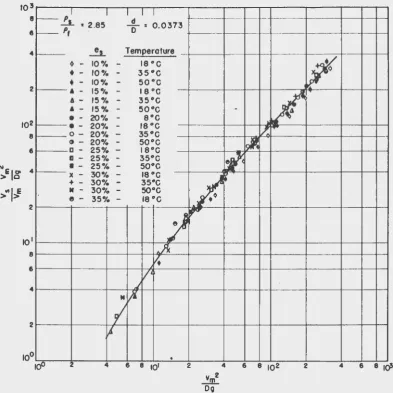
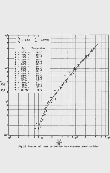
From2the tests ~onducted it was possible to plot a separate curve
of vs vm versus Vm for each of the five types of particles. These
vm Dg Dg ..V~Dv
curves, shown in Figs. 20 through 24, indicate that es, ' 1 · m and
/ I
~2 /
fr-·m do not affect the value of the velocity ratio beyond the limits
~ £
of experimental error. By introducing the paraneters, d and ( s, the
15
""71
five curves were combined and the equation of the resultant curve written as
where
This
B _ P
o.oL.
- (-(_S) •
r
f
can be rewritten in the form l
0.12 d'Cl60
f
s [13 do.
71(fl
s -1.28 v i B-1.00- vm2 -1.00/(-J ( _ ) (_) _ ) ( - ) ( - ) 1
D ( f D ,/ f Dg Dg
-v m 2
which shows more clearly the effect o~Dg on the ratio of the velocity
of the solid to the velocity of the ffilxture.
(23)
(22a)
In Table 2 the values of the dimensionless parameters and the range
of the tests for each group of particles are tabulated. The experimental
data collected fron the tests are tabulated in the Appendix.
VII.
DISCUS~IONThe major portion of this investigation was directed along experimental
lines, and equation (22) is the result of these efforts. This equation
indicates that, within the limi~s tested, the ratio of the velocity of
the solid to the velocity of the mixture is a function only of the geometry
of the particles and the conduit, the densities of the particles and the
fluid, and the velocity of the mixture. The fact that the concentration
and temperature do not influence the velocity ratio is obvious by the
absence of terms involving concentration or temperature dependent
103 8 8 4 2 102 8 6 ·N
'"101
4> 0
2 I 10 8 6 4 2
t - - p' I I d I I f - -- - - - -·-
-..:.1. • 2.85 0 = 0.0373
t - - pf
_!I_ Temperature ~
-
10%-
18 •c~
.
- 10%-
35•c.
-
10%-
50°C'
-
15% - 18°Clit
A - 15%-
35•c'
-
15"1. - 5o•c-.
-
20% - 9•c.
-
20% - I8°C:/.:
0 - 20% - 3s•c
<t - 20% - 5o•c
~
0 - 25% - 19•c
-a - 25% - 35•c
r¥<
I - 25% - 5o•c X - 30%
-
19•c;f.
+ -
..
30%-
35•c-
30%-
so•ce - 35% - 19•c
j
r
Ji<
v.
v
"
Ml/i
I
,J. •2 2 4 6 e 102 2
.!.JJl
oo
Fig. 20 Results of tests on 0.0114 Inch diameter glass particles.
[image:46.540.79.473.166.560.2]~
Is
1--·-
-.
pf 2.524 2 lo2 8 6 2 101 8 6 4 2
1 ·
-e,
v- 5% I ) - ro% f-· -· -10% ~- 10%
4 - 15% • -20%
r--o- 20%
'----()- 20%
D - 25%
~x- 30%
+- 30% _ N - 30o/e
ro0
ro0 2
-4 ISC-.586I
I I
~yd
~
0 • 0.111
";
~
.. --
f--Tem~eroture
r/
50 °C
reoc
i
35 ° c - ! - - -···-· r--50 °C
)~
18°C18°C 35°C
50°C "/Woo 35°C
+1 ~
reoc
If
35°C
50°C eJ
/
/
) / .) , · ·-6 8 101 2 4 6 8 102 2 4 6 8 lo'
Vm2
DO
Fio. 21 Results of tests on 0.0314- inch diameter oloss particles.
4
2
6
Nr;lo 4 ::>"10 101 8 6 4 2
- Ps I ld I I
= 7.50 = 0.0487
- pf 0
-v
-
es Temperature/
-~
-
1o•;. - 18 ~c•
-
10% - 35 •cA
-
15% - 18 •c- 4
-
15%- 35 •c,/
A
-
15%- so•c•
-
20%- 18 •c 0 - 20%- 35 •c- c t
-
20-t. - so •c1
_ o-
25%-
18 •c•
-
25%- 35 •c~·
-·
-
25% - so ·c 6X - 30%- 18~
£v
+
-
30%- 35•c-
..
-
30-t.- so•cIS.
- - ---e
-
35%- 19•c~J
e
-
35,. - 3s•c•
- 68.7-t.- 1a•c-·--
-./,
-~
-~r - -- ---- -~---·-··-· --- ·- --- ---;;
~:.·
,.
e
1/~·
" I
0
2 2 2
vm2
og
[image:48.540.83.470.52.660.2]6 4 2 6 2 101 8 6 4 2 ISC-586
~ I ~ I I
- - _s - - - -1----
---·-• 7.!50 : 0.245
Pt 0
- - - - -- --- ---- ~----
--.---
- -
es Temperature - - ----y - !5 •;.
-
1e·•c 17-
s•;.-
35•c'
-
5%-
5o•c··-·-- --~ -10%
-
1e•c - ----•
- 10%-
35•c•
-10%-
5o•cj -15% - 1e•c
6 - 15% - 35•c
---a
-
15%-
5o•c - -~-
·
-20% - 1e•c - ---- .-------+'f)(
0 -20% - 35•c 6~
- -() -20% - 5o•c
'"
(_
D - 25% - 1e•c 0
_ a -25%
-
35•c-:t.
-•
-25%-
5o•c M GlX - 30% - 1e•c
+ -30%
-
35•c !M -30%
-
5o•c 6f - - -e -35% - 1a•c
.;;
e -35% - 35•c e
1--- - ----
--()
lO"
- - - --->----
,
•ye
- -- - --- --- --- ---;~ 17/
2 4 6 8 10' 2 4 6
x
Og
Fig. 23 Results of tests on 0.0722- inch
43
6
-- - - -f
--·
/---
--- ~r
---- --- - _X_ _
~·
~:#
()--
---•
~ tp - -
--- ---1---f---
f--- f-
---·-- ---
-2 4 6 e
1rr
[image:49.534.56.464.52.653.2]lOS
•
•
2
101
•
6
2
r -
~
! d'
I I ,.- · . 11.3 0 . 0.1!56 n
t - - - Pf
m+
v
,.x~__!!.._ Tem~erature
-~
•
- 10 .,. - 35•c"
- 1!5 .,. - 1e•c4 - 15 .,. - 35•c
•
-20%-
1e•c.V
0 - 20.,./o - 35•c
() -20% - 5o•c
0 -25% - 1e•c II - 25% - 35•c
I -25% - 5o•c Si{~'
X -30% - 1eoc
'
I•+ -30% - 35•c ...
M -30% - 50°C
a,j
~e -35% - 35°C
e -35% - 50°C
f
II -40% - 1e •c
I
II ~4Q% - 35° cIll -40% - 50° c
r - v -45% ~
35° c
·;r
J
~
,,
f
I
0
t
1
2
Vm2
6 8 ld 2 4 2 4 6 8 lOS
DQ
Table 2
Particles tested and range of the tests of velocity ratio
Particle Particle Trbe d ~..:-s
diameter dianeter
I5
r" f e Rao~;eof te:::lts
vm2 ·Temperature
inches irches \ dS
oc
/0
Dg
Glass
0.0114
0.306
0.0373
2.85
8.0 - 58.2
2.00 - '319.
7.5 - 52.7
H(/)
0
0.0314
0.283
2.52
4.9 - 32.3
5.89 - 641.
IGlass
0.111
13.8 - 52.8
\Jl.co
0'-Steel
0.0149
0.306
0.0487
7
.so
7.4- 34.7
2.24 - 376.
14.0 - 51.8
Steel
0.0722
0.295
0.245
7.50
2.9 - 38.4
3. 73 - 591.
13.6 - 52.3
Lead