Article:
Liu, R., Van Vliet, D. and Watling, D.P. (2006) Microsimulation models incorporating both
demand and supply dynamics. Transportation Research A, 40 (2). pp. 125-150. ISSN
0965-8564
https://doi.org/10.1016/j.tra.2005.05.003
[email protected] https://eprints.whiterose.ac.uk/
Reuse See Attached
Takedown
If you consider content in White Rose Research Online to be in breach of UK law, please notify us by
White Rose Research Online
http://eprints.whiterose.ac.uk/
Institute of Transport Studies
University of Leeds
This is an uncorrected proof version of a paper originally published in
Transportation Research A. It has been peer reviewed, but does not include the
final publisher’s corrections.
White Rose Repository URL for this paper:
http://eprints.whiterose.ac.uk/2488/
Published paper
Liu, R.; Van Vliet, D.; Watling, D.P. (2006)
Microsimulation models incorporating
both demand and supply dynamics
- Transportation Research. Part A: Policy &
Practice 40(2) pp125-150
UNCORRECTED
PROOF
2
Microsimulation models incorporating both demand
3
and supply dynamics
4
Ronghui Liu
*, Dirck van Vliet, David Watling
5 Institute for Transport Studies, University of Leeds, Leeds LS2 9JT, UK
Received in revised form 25 April 2005
8 Abstract
9 There has been rapid growth in interest in real-time transport strategies over the last decade, ranging
10 from automated highway systems and responsive traffic signal control to incident management and driver
11 information systems. The complexity of these strategies, in terms of the spatial and temporal interactions
12 within the transport system, has led to a parallel growth in the application of traffic microsimulation models
13 for the evaluation and design of such measures, as a remedy to the limitations faced by conventional static,
14 macroscopic approaches. However, while this naturally addresses the immediate impacts of the measure, a
15 difficulty that remains is the question of how the secondary impacts, specifically the effect on route and
16 departure time choice of subsequent trips, may be handled in a consistent manner within a microsimulation
17 framework.
18 The paper describes a modelling approach to road network traffic, in which the emphasis is on the
inte-19 gratedmicrosimulation of individual trip-makersÕ decisions and individual vehicle movements across the
20 network. To achieve this it represents directly individual driversÕ choices and experiences as they evolve
21 from day-to-day, combined with a detailed within-day traffic simulation model of the space–time
trajecto-22 ries of individual vehicles according to car-following and lane-changing rules and intersection regulations.
23 It therefore models both day-to-day and within-day variability in both demand and supply conditions, and
24 so, we believe, is particularly suited for the realistic modelling of real-time strategies such as those listed
25 above. The full model specification is given, along with details of its algorithmic implementation. A number
26 of representative numerical applications are presented, including: sensitivity studies of the impact of
day-to-27 day variability; an application to the evaluation of alternative signal control policies; and the evaluation of
0965-8564/$ - see front matter Ó2005 Published by Elsevier Ltd.
doi:10.1016/j.tra.2005.05.003
*Corresponding author. Tel.: +44 113 343 5338; fax: +44 113 343 5334.
E-mail address:[email protected](R. Liu).
www.elsevier.com/locate/tra
UNCORRECTED
PROOF
28 the introduction of bus-only lanes in a sub-network of Leeds. Our experience demonstrates that thismod-29 elling framework is computationally feasible as a method for providing a fully internally consistent,
micro-30 scopic, dynamic assignment, incorporating both within- and between-day demand and supply dynamics.
31 Ó2005 Published by Elsevier Ltd.
32 Keywords: Microsimulation; Network; Route choice; Variability; Real-time strategies
33
34 1. Introduction
35 Recent years have seen a massive increase in real-time advanced technological strategies
36 designed, for example, to reduce congestion, improve network efficiency, promote public trans-37 port use, decrease pollution and/or increase road safety. At the network-wide level, these include: 38 responsive, optimised traffic signal control, e.g. SCOOT (Hunt et al., 1981); congestion-based
39 road pricing (Oldridge, 1990); dynamic route guidance/information and variable message signs
40 (Emmerink and Nijkamp, 1999); congestion management strategies, e.g. freeway ramp-metering, 41 gating (Papageorgiou et al., 1989); public transport priority measures such as responsive bus sig-42 nal controls (Quinn, 1992), bus lanes and guided bus schemes (Liu et al., 1999).
43 A general property of all these strategies is that they both respond to—and in turn influence—
44 prevailing congestion levels, rather than being designed on the basis of long-term average condi-45 tions. That is to say, the variation in traffic conditions is just as important a consideration as the 46 mean. Variabilities include the temporal distribution of flows, as well as the variation in travel 47 times and delays both within and between days. It includes not onlynaturalvariability associated 48 with normal trip making decisions but alsounnaturalvariability associated with incidents or acci-49 dents. In order to evaluate these systems and to determine the best strategy for implementation, it 50 is crucial to have a reliable evaluation model that fully incorporates the effects of variability. In 51 addition, since these strategies all must be implemented within the wider transport system, it is 52 important that such an evolution model reflects thenetwork effects of any measures.
53 The analysis of traffic networks has traditionally been based on WardropÕs equilibrium principle 54 (Wardrop, 1952), predicting a long-term average state of the network. Such a model assumes stea-55 dy-state network supply and demand conditions from day-to-day and within different periods of a 56 day, and therefore has great difficulty in representing the dynamics of the transport systems and 57 many of the above mentioned contemporary transport policies whose major purpose is to deal with 58 variability in demand and network traffic conditions. In addition there is strong evidence that, by 59 ignoring most sources of day-to-day and within-day variabilities, conventional equilibrium models 60 tend to over-estimate network performance and therefore to produce biased results (Mutale, 1992).
61 Partly in response to these deficiencies, enormous advances have been made in the way in which
62 traffic networks may be modelled. Among which is the advances in the use of microsimulation 63 technique in modelling drivers and driver behaviour in transport networks. By explicitly repre-64 senting the individual entities, i.e. the people and vehicles, that act and interact in a transport net-65 work system, microsimulation modelling provides an extremely flexible framework whereby 66 disaggregated, behaviour-based research can be incorporated and tested.
67 A large number of traffic microsimulation models have been developed in order to study
UNCORRECTED
PROOF
69 are studies of:automated highway systems, such as lane routing (Eskafi et al., 1995; Lee and Lee, 70 1997), merging control (Ran et al., 1999; Hidas, 2002), ramp-metering (Hasan et al., 2002) and the 71 integrated control of access, lanes and routes (Ben-Akiva et al., 2003); automatic vehicle control72 systems (Chang and Lai, 1997) such as adaptive cruise control (Marsden et al., 2001; Suzuki
73 and Nakatsuji, 2003) and intelligent speed adaptation (Liu and Tate, 2004);traffic management
74 measures, ranging from bus priority schemes (Quinn, 1992; Liu et al., 1999) to tollbooth design
75 (Huang and Huang, 2002), pedestrian facility design (Liu et al., submitted for publication) and 76 responsive traffic signal systems (Kosonen, 2003; Niittyma¨ki and Turunen, 2003; Bullock et al., 77 2004);Incident Management Systemsincluding incident recognition (Mussa et al., 1998), incident 78 detection (Khan and Ritchie, 1998; Sheu, 2004), and incident response strategies (Sheu and Ritch-79 ie, 2001; Cova and Johnson, 2003); real-time driver information systems (Hu and Mahmassani, 80 1997; Dia, 2002; Adler et al., 2005; Rossetti and Liu, 2005); traffic flow stability analysis ( Cha-81 kroborty and Kikuchi, 1999; Huijberts, 2002; Davis, 2003; Bham and Benekohal, 2004); and 82 theprediction of environmental impacts, including exhaust emissions (Yu, 1998), energy consump-83 tion (Ambrosino et al., 1999), and safety (Ko¨ll et al., 2004).
84 It is noticeable that a great majority of these applications have focused on problems of a short-85 term forecasting nature, where microsimulation is able clearly to demonstrate its advantages over 86 static, macroscopic approaches in estimating theimmediatetraffic flow impacts of some measure. 87 However, in the present paper we are particularly interested in the potential for microsimulation 88 as a medium-term transport planning tool. In this latter case, it is crucial to consider thesecondary
89 effects1 caused by drivers changing their travel decisions on subsequent trips in response to their 90 new experiences of traffic conditions. Thus, for example, the implementation of a new responsive 91 traffic signal system at an intersection may lead to reduced delays in the short term, but in time 92 (over a period of days and weeks) this may lead to traffic diverting from alternative routes or 93 changing their time of trip departure, leading to a medium-term change in the magnitude and pro-94 file of the flows that impinge on that intersection. In spite of all the criticisms of the static equi-95 librium paradigm, it is the ability of such an approach to deal with both the immediate and 96 secondary effects that has led to its popular use in transport planning. If microsimulation is also 97 to take its place as a mainstream approach to transport planning, it must be able to address such 98 secondary effects.
99 How have microsimulation approaches been used to address these secondary effects? Three
100 main approaches may be identified. In the first approach, the secondary effects are neglected
101 (e.g.Laird et al., 1999). This might lead one to conclude that, therefore, no secondary effects will 102 occur in the model, but this may not be quite true. In particular, if the microsimulation input data 103 requires turn probabilities to be input at each intersection (rather than, say, complete routes to be 104 defined), thenÔroutesÕare implicitly reconstructed by making Monte Carlo draws for each vehicle 105 according to these turn probabilities. If some control measure is then applied which affects the
106 sequencing of vehicle arrivals, then there will be an impact on the sampled turn proportions
107 due to the effective change in sequence of the random numbers generated. Thus, even though 108 no behavioural model is supplied to represent the secondary effect, an apparent effect may occur 109 simply due to Monte Carlo noise. It is difficult to justify such an impact as desirable, since the
1 The term
UNCORRECTED
PROOF
110 modeller has no control over it, and indeed both anecdotal and theoretical evidence exists to sug-111 gest that such turn-based definitions may lead to implausible cycles (vehicles re-visiting the same 112 link a number of times) of arbitrary length (Akamatsu, 1996).113 In the second approach, the secondary effects are predicted by using a coarser model which is
114 either run once in stand-alone mode prior to the microsimulation (for example, Montero et al.,
115 2001, propose the use of a static equilibrium model, with the equilibrium turning fractions then 116 input as turn probabilities to the microsimulation), or is based on some aggregated feedback loop 117 from the microsimulation (Fellendorf and Vortisch, 2000; Barcelo´ and Casas, 2004). In neither 118 case are the secondary-level decisions made on the basis of consistent assumptions and aggrega-119 tion levels with the microsimulation, and so one is open to the same criticisms levelled at the static 120 equilibrium approaches.
121 The third approach is to use some consistent mechanism to feedback the travel experiences at
122 the microscopic level and simulate individual trip choices (Liu et al., 1995; Nagel and Barrett, 123 1997; Hu and Mahmassani, 1997). In this approach, then, one effectively defines a dynamic pro-124 cess that explains driversÕday-to-day learning and trip-to-trip travel choice adjustments. A further 125 advantage of this approach is that one can avoid the problems of turn-probability based
defini-126 tions (noted above), by requiring the day-specific inputs to the microsimulation to be complete
127 paths traversed at particular departure times, the paths and departure times both being selected
128 by the dynamic process model explaining the day-to-day adjustments. The price paid for such 129 an approach is, however, a much more complex model to interpret, with complex issues of con-130 vergence, stability and even existence of attractive states to handle.
131 In spite of these latter comments regarding model complexity, it is our belief that the third ap-132 proach noted above is the most appropriate for taking microsimulation into mainstream transport 133 planning, since it offers both an integrated (single model) and consistent (all decisions and expe-134 riences made at individual level) approach to the problem. This paper describes a particular model 135 framework based on such an approach. The model, code named DRACULA (Dynamic Route 136 Assignment Combining User Learning and microsimulation), integrates a microsimulation of 137 individual drivers day-to-day learning and route choice model with a traffic microsimulation mod-138 el of the car-following and lane-changing nature. In combination they model the evolution of the 139 traffic system over a representative number of days so that both within-day and between-day vari-140 abilities are included.
141 The structure of the paper is as follows. The general structure of the DRACULA microscopic
142 framework of day-to-day dynamic network models is introduced in Section 2. The methodological 143 and algorithmic aspects of the day-to-day evolution model (Section 3) and the within-day traffic 144 simulation model (Section 4) are then described in detail. A brief description of the DRACULA 145 software design and implementation is given in Section 5. Potential applications of such a model 146 framework and demonstrations of its applicability in tests of realistic policy measures are given in 147 Section 6, followed by concluding remarks (Section 7).
148 2. DRACULA model structure
149 As with conventional equilibrium models the DRACULA approach begins with the concept of
con-UNCORRECTED
PROOF
151 trast with conventional models, in DRACULA both the demand and supply sub-models are 152 based on microsimulation and both evolve from day-to-day. In DRACULA, trip makers are indi-153 vidually represented and their daily route choices (demand) are made based on their past experi-154 ence and their perceived knowledge of the network conditions. Individual vehicles are then moved 155 through the network (supply) following their chosen routes according to rules governing car-fol-156 lowing, lane-changing and intersection control. The demand stage predicts the level of individual 157 demand for daynfrom a full population of potential drivers and the supply model for dayn deter-158 mines the resulting travel conditions. The costs experienced by drivers are then re-entered into 159 their individualknowledge baseswhich in turn affect the demand model for dayn+ 1. The process 160 continues for a pre-specified number of days. The overall structure of the framework and the 161 interaction among its various sub-models are illustrated in Fig. 1.162 The framework combines a number of sub-models of traffic flow and driversÕchoices for a given
163 day with a day-to-day driver learning sub-model. In its most general form it has the following 164 structure although, as we shall discuss later, certain alternative methods or simplifications are pos-165 sible within most stages.
166 1. [Input data] Load data on network representation and origin–destination trip matrix.
167 2. [Population generation] Establish a population of potential drivers with individual
characteristics.
169 Day-to-day (demand) loop:
170
171 3. [Initialisation—Part I] Set initial driver perceptions for each link in the network. Set day
counter k= 1.
173 4. [Daily demand] Select the total day-kdemand for each origin–destination pair according to
some given probabilistic rules.
175 5. [Departure time choice] Individuals travelling on the day adjust their departure time to travel based on previous experience.
177 6. [Route choice] Each individual travelling on the day chooses a route based on their current
perception of traffic conditions and previous experiences. The travel time component of the cost is based on the individualsÕdeparture time and their predicted arrival times at each link/ turn.
181 7. [Supply variability] Select global network supply condition for day k prior to loading by
some given probability laws to simulate effects such as weather and lighting conditions.Local
variations in network conditions (such as road works, incidents occurring on the day) are also specified.
185 Within-day (supply) loop:
186
187 8. [Traffic loading] A microscopic simulation of traffic conditions on daykis carried out given the choices and supply variability above. Drivers experience within-day variable link and turn travel times for the route and departure time they have chosen.
UNCORRECTED
PROOF
(b) [Vehicle generation] Vehicles enter the network at their chosen departure time. Each vehicle is assigned a set of individual characteristics.
(c) [Vehicle movement] Each vehicle follows the pre-specified route. Their speeds and posi-tions are updated according to car-following, lane-changing and gap-acceptance rules, and traffic regulations at intersections.
(d) [Traffic control update] For each signalised junction, update the stage change-over clock according to desired signal plans (fixed plans or responsive). Check if any incident is to start or to finish.
(e) [Data collection] Individual driversÕexperience within-day are stored. Aggregated mea-sures such as queue length, travel time, speed, flow, emissions, fuel consumption are recorded for every turn, link, route, and O–D pair, and for the whole network.
(f) [End of day] If all drivers have finished their journey, terminate the day; otherwise
increment the simulation clock and return to step 8b. 204
INPUT DATA Network Representation
Trip Matrix
POPULATION GENERATION
DEPARTURE TIME, ROUTE SELECTION
TRAFFIC MICROSIMULATION DAILY
DEMAND
DRIVER LEARNING
Individual trip plan: route, dept-time List of individuals to
travel on day k
New perception of the network
Individual travel experience on the day DAY -TO-DAY EVOLUTION
SIMULATION OUTPUT Distributions of link and
route flows, costs
UNCORRECTED
PROOF
205 9. [Learning] At the end of dayk, drivers update their perceptions based on their experiences of206 link and turn travel times on the day.
207 10. [Stopping test] If some stopping condition is satisfied, terminate; otherwise increment the day
208 counter and return to step 4.
209
210 Note that this process will not converge to a single equilibrium point but will continue to vary 211 from one day to the next. Instead, our objective is to determine the probability distribution of 212 individual day-to-day states, appealing to the theory of stochastic processes (Cascetta, 1989; Can-213 tarella and Cascetta, 1995; Watling, 1996; Hazelton and Watling, in press).
214 Similar models of this day-to-day structure have been considered previously byAlfa and Minh
215 (1979), Ben-Akiva et al. (1986), Vythoulkas (1990), Emmerink et al. (1994), Nagel and Barrett 216 (1997), Hu and Mahmassani (1997), though generally with the day-to-day evolution represented 217 as a deterministic process, with the aim to converge to a fixed point.
218 Details of the functionality of steps 2–7 and step 9 are discussed in Section 3. Section 4 intro-219 duces the traffic microsimulation model used in step 8.
220 3. Day-to-day evolution of travel demand and network conditions
221 3.1. Modelled population
222 In principle, the modelled population can include all the potential drivers in the study area.
223 Each individual member of this population has certain characteristics (such as household origin, 224 work place, car-ownership status, driving style, etc.) and a history filein which the accumulated 225 experience of previous choices and travel conditions encountered is stored. Equally the vehicle 226 they drive will have certain fixed characteristics such as vehicle size and engine type which do 227 not change from day-to-day. As far as feasible the distribution of characteristics should match 228 as closely as possible that of the area being modelled.
229 In practice, however, simplifications and compromises will need to be made. More
pragmati-230 cally therefore we aim at generating a population whose trip making behaviour at the aggregate 231 day-to-day level matches the averages and variances observed in real life. In our applications, the 232 population is derived from an existing conventional trip matrix Tijfrom origini to destinationj. 233 We then assume (see also Section 3.2 below) that the day-to-day variability in the number of trips 234 may be described by a normal distribution whose mean isTijand whose variance isb2dT2ij where 235 bd> 0 is a user-set coefficient of demand variation. Hence the demand for ijtrips on day kis:
tðijkÞ¼NorðTij;b2dT2ijÞ ðtruncated at zeroÞ ð1Þ
239 We define our population of potentialijtravellers to beTmaxij , the pragmatic maximum number of 240 trips generated by Eq.(1). Although the maximum of Eq.(1)is effectively infinite, in practice we use:
Tmaxij ¼Tijþ3bdTij ð2Þ
UNCORRECTED
PROOF
246 model run. The most obvious application of this is in a before-and-after study of a scheme, in 247 which the initialisation of theÔafterÕrun is based on the final conditions of theÔbeforeÕrun. Sim-248 ilarly, the initialhistoriesof drivers—i.e. their remembered experiences on the network—may be 249 set to be their accumulated experiences in the previous run.250 In addition todrivers, the modelled population also includes elements such as buses following 251 fixed routes, for which clearly route choice and aknowledge baseare not issues. They will, how-252 ever, require their own appropriate vehicle characteristics.
253 3.2. Day-to-day demand
254 On any particular day within the evolution of the model each member of the population makes
255 a decision as to whether to travel or not. In principle the decision could—and should—be based 256 on the individual characteristics of that member of the population, so as to differentiate between 257 regular commuters and one-off shopping trips and to include elements of their knowledge base. In 258 practice a more pragmatic approach has been used whereby individual decisions are constrained 259 by the predicted daily trips for their particular origin–destination pair.
260 Thus for each origin iand destination j we:
261 (1) select the mean demand level appropriate to dayk, denoted tðijkÞ, from Eq.(1); 262 (2) form the probabilitypðijkÞ¼tijðkÞ=Tmaxij ;
263 (3) each potential traveller then independently chooses to travel on daykwith probabilitypðijkÞ.
264
265 Note that clearly, any reference to driversÕhistories or choices made during the simulation re-266 lates to the fixed pool of potential travellers who keep their identification through the simulation, 267 rather than the day-to-day varying pool of individuals who actually make a journey through the 268 network.
269 A generalisation of this method is also permitted, in which different user classes are defined,
270 which differ only in their propensity to travel (representing, for example, shopping trips which 271 may be made less frequently than journey-to-work trips).
272 3.3. Departure time distribution
273 The choice of departure time within DRACULA may be handled in a number of different ways.
274 The default and simplest method is to randomly assign a desired departure time for each potential 275 driver in the modelled population according to some departure time profile. When drivers choose 276 to travel on daynthey will depart at their desired departure time, independent of their experience 277 and route choice. The departure time profile could be flat or distributed probabilistically accord-278 ing to some user-specified distribution, for example, a step function over time slices.
UNCORRECTED
PROOF
285 (a) preferred arrival time at the destination, aijm;286 (b) trip time from the previous daytðijmkÞ; and 287 (c) departure time on the previous daydðijmkÞ.
288
289 For example,aijmcould be randomly drawn at the start of the simulation from a specified time
290 profile as in the first method.
291 The difference between the desired and actual arrival time on day kis then:
dijmðkÞ ¼dðijmkÞ þtijmðkÞ aðijmkÞ ð3Þ
294 The driver is assumed to (independently between days and from other drivers) be indifferent to
295 a lateness ofemt
ðkÞ
ijm, which is modelled as in proportion to the actual travel time. The proportionem 296 for individual m is drawn from a uniform [0,e] distribution, wheree is a user-defined maximum 297 lateness tolerance factor and anem= 0 means zero tolerance to lateness. Hence, we define the per-298 ceived lateness as:
DðijmkÞ ¼dðijmkÞ emtðijmkÞ ð4Þ
301 If DðijmkÞ >0, the users adjust their departure time so that the perceived lateness would be zero if 302 yesterdayÕs trip time were repeated, then,
dijmðkþ1Þ¼dijmðkÞDðijmkÞ ð5Þ
306 Otherwise,
dðijmkþ1Þ¼dðijmkÞ ð6Þ
309 Thus, in the model described, no early arrival correction is made, but this is readily incorporated 310 by settingdðijmkþ1Þaccording to Eq.(5)regardless of the sign ofDðijmkÞ. The flexibility of the framework 311 enables a more general departure time choice to be implemented easily at a later stage.
312 3.4. Route choice
313 By default, each driver travelling on a particular day chooses their minimum perceived
gener-314 alised cost route based on the traditional concept of utility maximisation that underlies virtually 315 all current traffic assignment models. The key difference is in the concept ofutilityorcostwhich is 316 now an attribute that evolves and varies over days. At the start of any day, each individual forms 317 a perceived cost at a linear combination of relevant attributes (travel time, distance, generalised 318 cost, tools, etc.). For those attributes that are not static, primarily travel time, the travel time used 319 for each link is the one that emerges from the learning process described in Section 3.5 based on 320 that driverÕs individual history.
321 An alternative choice model implemented in DRACULA is theboundedly rational choice, based
322 on the work of Mahmassani and Jayakrishnan (1991). This model assumes that drivers will use
323 the same (habit) route as on the last day in which they travelled, unless the cost of travel on 324 the minimum cost route issignificantlybetter than that on their habit route. The threshold is that 325 a driver will use the same route unless:
UNCORRECTED
PROOF
328 whereCp1andCp2are costs along the habit and the minimum cost routes respectively,gandsare329 global parameters representing the relative and the absolute cost improvement required for a 330 route switch.
331 These rules are only intended as an example of the range of rules that could possibly be imple-332 mented in a flexible approach such as DRACULA. Alternative behavioural rules that could be 333 provided in the future include the concept of risk minimization, with drivers perceiving cost vari-334 ances as well as means.
335 The route choices are made and fixed before the trips start; drivers follow their chosen routes 336 through the network to their destinations and will not (within the current state of model develop-337 ment) make en-route diversion when, e.g., encountering congestion.
338 3.5. Learning
339 After each journey individuals use their experienced travel times on the links used on that jour-340 ney to update their perceived link travel times according to the following conditions:
341 (a) experiences more than Mdays old are forgotten; and
342 (b) the perceived travel cost is the average of (at most) the lastN remembered experiences on
that link. 344
345 HereMandNare global parameters set at the start of simulation, although their effect will be 346 specific to each individualÕs experience. It may reasonably be argued that these parameters should 347 be allowed to vary with the driver and/or trip type, and indeed this may be incorporated in the 348 framework described.
349 Generally, it is expected that N will be the main parameter affecting perceived cost; M is
350 intended mainly as a device for drivers to ultimately forget a single bad experience of a link which 351 may occur particularly in the atypical, initial warm-up days. Therefore, it is expected thatN<M.
352 3.6. Supply variability
353 The effect of day-to-day variability in network conditions is represented at two levels. The
354 global variabilityrepresents the effects of weather, daylight, etc., on the network. It is represented
355 in the model by a variable link cruise speed drawn from a normal distribution whose mean isVl 356 and whose variance is b2sV2l where bs> 0 is a coefficient of global supply variation. Hence the
357 cruise speed for linkl on day kis:
vðlkÞ¼NorðVl;b2sV 2
lÞ ðtruncated at a minimum speedÞ ð8Þ
360 Local variabilityis in the form of incidents (e.g., breakdowns or road closures) which may occur
361 one day but not another. This is represented before loading by specifying the location and dura-362 tion of the incidents.
UNCORRECTED
PROOF
366 4. The traffic simulation367 The traffic model in DRACULA is a microscopic simulation of the (pre-specified) individual
368 vehiclesÕ movements through the network. Drivers follow their pre-determined routes and
369 en-route encounter signals, queues and interact with other vehicles on the road. A large number
370 of such microscopic vehicle models have been developed in the past at varying levels of complexity 371 and network size (e.g. in some the network is effectively a single intersection)—see a review by
372 Algers et al. (1997). An essential property of all such models is that the vehicles move in real-time 373 and their space–time trajectories are determined by, e.g., car-following and lane-changing models 374 and junction controls such as signals.
375 The traffic simulation model developed for DRACULA is based on fixed time increments; the
376 speeds and positions of individual vehicles are updated at an increment of 1 s. Spatially, the sim-377 ulation is continuous in that a vehicle can be positioned at any point along a link. The simulation 378 starts by loading the simulation parameters, network description including global and local var-379 iability and trip information (i.e. the demand and routes determined by the demand model). It 380 then runs through an iterative procedure at the pre-defined time increments, within which the 381 tasks in steps 8(a)–(f) described in Section 2 are performed.
382 4.1. Network representation
383 The network is represented by nodes, links and lanes. A node is either external, where traffic
384 enters or leaves the network, or an intersection. All major UK intersection types are modelled; 385 these include priority give way, traffic signal controlled intersections, roundabouts, and fully or 386 partially signalised roundabouts. A link is a directional roadway between two nodes and consists 387 of one or more lanes. A link is specified by its upstream and downstream nodes, cruise speed, 388 number of lanes, and turns permitted to other outbound links from the downstream node. Vehi-389 cles move in lanes and follow each other according to the car-following rules. They travel through
390 intersections alonginter-laneswhich are smoothed curves connecting the inbound and outbound
391 lanes. The crossing point of two inter-lanes is a conflict point. Various access restrictions such as 392 one-way streets and reserved lanes, and geometric designs such as flared approach to intersections 393 (where an approach is widened into separate turning lanes) are represented.
394 4.2. Vehicle generation
395 Vehicles are individually characterised, including a technical description of the vehicle (vehicle 396 type, length, maximum acceleration and deceleration capability) and behaviour of the driver 397 (reaction time, stopping distance headway, acceptable time gap, desired speed, desired accelera-398 tion and deceleration). These characteristics are randomly sampled from truncated normal distri-399 butions representative of that type of vehicle:
Pu ¼NorðPu;b2vP2uÞ ðtruncated at P min u and P
max
u Þ ð9Þ
UNCORRECTED
PROOF
404 coefficient of variation of vehicle characteristics which can be made vehicle-type specific. For 405 example, there may be greater variability in car driversÕ desired speed and acceptable gap than 406 those of drivers of large goods vehicles. The characteristics for each vehicle are chosen at the start 407 of a simulation run and they remain the same for the same vehicle from one day to the other. Pub-408 lic transport vehicles are represented with additional information such as service number, service 409 frequency, bus stops en-routeand passenger demand (Liu et al., 1999).410 The default values (as used in the numerical results reported in Sections 6.3–6.5) are based on a
411 number of sources including May (1990), Institute of Transportation Engineers (1982), Gipps
412 (1981). A discussion on the choice of parameter values for microsimulation models and their 413 impact on model results is presented inBonsall et al. (in press).
414 4.3. Vehicle movement
415 Vehicles are moved in real-time and their space–time trajectories are determined by their
416 desired movements, response to traffic regulations and interactions with neighbouring vehicles 417 according to car-following and lane-changing rules and simulation of conflicts at intersections. 418 A detailed description of the vehicle movement simulation model incorporated in DRACULA
419 can be found inLiu (2005). The key driving behaviour modelled is presented below.
420 4.3.1. Car-following model
421 The car-following model represents the longitudinal interactions among vehicles in a single
422 stream of traffic. It calculates the following vehicleÕs speed and acceleration in response to stim-423 ulus from the preceding vehicle. Depending on the relative distance to the preceding vehicle, 424 the following vehicle is assumed to be in one of three different following regimes: free-moving, 425 normal following, or close-following.
426 When a vehicle is the leading vehicle in a platoon, or is long way away from its downstream
427 intersection, it is assumed that the vehicle can accelerate or deceleratefreelyin order to maintain 428 its desired speed.
429 When the space headway becomes shorter, the following vehicle will enter thenormal following
430 regime and will take a controlled speed derived from a linear function of the relative speed and 431 distance to the preceding vehicle. When the space headway gets very small and the vehicle is de-432 scribed as inclose-following regime, the driver will prepare to stop in case the preceding vehicle
433 brakes suddenly. A stopping distance based car-following model as proposed by Gipps (1981)
434 is used here to describe such close-following regime.
435 4.3.2. Lane-changing model
436 The model firstly identifies the reasons for a lane-changing desire. The following reasons or
437 types are considered:
438 (a) bus stopping at bus stops;
439 (b) avoiding an incident (e.g. accidents, road works, parked vehicles);
440 (c) making junction turning movement at the immediate downstream intersection;
441 (d) moving into a lane reserved for their type, or avoiding a restricted-use lane;
UNCORRECTED
PROOF
443 (f) giving way to a merging vehicle or to a bus merging from a bus lay-by; or
444 (g) anticipating a lane-changing need of type (a), (c) or (d) in a downstream link. 445
446 The first three types are mandatory, i.e. the lane-changing has to be carried out by a certain
447 position on the current link, for example the location of the bus stop. The other types are
448 discretionary; whether such a discretionary lane-changing can be carried out depends on the
449 actual traffic conditions. For example, a vehicle would only change lane to gain speed if the speed 450 offered by the adjacent lane issignificantlyhigher than that on their current lane. The threshold is 451 a behavioural variable that can be calibrated to the observed local behaviour.
452 Once a lane-changing desire is triggered and the target lane selected, a gap-acceptance model is 453 used to find the gaps in the target lane which are acceptable to the driver wishing to change lanes. 454 A variable critical gap is modelled to reflect the phenomenon of impatient drivers for whom the 455 critical gap decreases with each passing gap (e.g.Kimber, 1989; Taylor et al., 2000). The stimulus 456 required to induce the decrease of critical gap is modelled as the time spent in searching for accept-457 able gaps. A minimum gap is used to set a lower boundary to the gap-reduction formulation.
458 4.3.3. Intersection simulation
459 In the model, vehicles start to react to traffic controls (traffic signals or give way sign) at a 460 downstream intersection when they reach a certain distancedsto the intersection.dsis used to rep-461 resent both the physical sight distance to the intersection and the sensitivity of drivers to intersec-462 tion control. Only the lead vehicle in a platoon reacts to intersection control; the following 463 vehicles follow the preceding ones according to car-following rules until they become the lead 464 vehicle.
465 At traffic signal controlled intersections, the model tries to take into account some of the unsafe 466 driving behaviour such as adopting a smaller headway when passing through the green phase, 467 passing traffic signals at amber or even at the start of red. The right-turning (for drive on the left) 468 vehicles (the number of these vehicles is dependent on the size of the junction) who needs to give 469 way to opposing straight-ahead vehicles can wait into the middle of the junction for a gap to 470 cross.
471 For a give way intersection, the model uses a visibility parameter to represent the geometric
472 openness of a junction and to model the phenomenon whereby, instead of stopping by the stop 473 line, some drivers may even accelerate to join in or to cross the major flow if they can see the sit-474 uation on the major road. The critical gap decreases as the time a driver spent waiting for an 475 acceptable gap increases.
476 Unlike the common method of representing roundabouts as series of one-way links, the model
477 represents a roundabout as a single node with a circular link around it. Vehicles approach a 478 roundabout as though approaching a priority junction: get into the correct lane for its junction 479 turning and give way to circulating traffic on the circular link.
480 4.4. Simulation outputs
481 To measure the performance of a network, the simulation provides summary statistics on the
UNCORRECTED
PROOF
484 the second-by-second individual vehiclesÕlocations and speeds. The model also provides point- or 485 loop-based detector measures on headway distribution, flow, occupancy and speed. For each bus 486 service, the model summarises the means and variances of total journey time and journey time 487 between stops; these measures can help distinguish service delays due to traffic congestion from488 those due to poor management. A graphical animation of the vehiclesÕ movements can also be
489 shown in parallel with the simulation, giving the user a direct view of the traffic conditions on 490 the network.
491 A clear distinction is made between the performance of a network and costs associated with a
492 given demand (Liu, 2005). The performance of a network or a single link can be measured in
493 terms of vehicle-km and vehicle-hour travelled in a defined period. These are the engineering 494 descriptions of the performance of the link or a network at a given point in time or over a given 495 time period, and can be used to estimate the link or network equivalent of speed–flow relation-496 ships. The performance measures can be obtained by dividing the simulation period into a number 497 of equal performance periods and aggregating the parts of the vehicle trajectories within each 498 period.
499 The supply costs reflect the costs experienced by a driver using the network at a given level of 500 demand; they can be used to describe the way in which costs of using a network rise as demand-501 levels increase. Since any journey through a network will pass through a number of different traffic 502 states and the costs incurred will be affected by both the journey length and the route taken, as 503 well as by the impacts of other demands on the network both at that time and in earlier time peri-504 ods. In order to measure these costs, individual vehicles need to betrackedthrough the network 505 and their origin–destination trajectories summarised. The summation can be done either over a
506 departure time period or an arrival time period where all vehicles departed or arrived during the
507 period respectively are summarised. In DRACULA the departure time aggregated supply mea-508 sures are recorded.
509 5. Implementation
510 DRACULA has been developed as a flexible framework through modular implementation of
511 its sub-models. We described in Sections 3 and 4 the most general formulation of the demand and
512 supply models. At its most detailed level, DRACULA represents individual driversÕday-to-day
513 choice making processes and individual vehiclesÕmovements through a network; this version of
514 the model is hereafter called thefull model.
515 In practice, however, it may be desirable to run the model with a number of simplifications.
516 Thus, the traffic supply model may be based on a more conventional static network model with 517 macroscopic flow–delay functions but with variable parameters such as link capacity, while the 518 demand model is based on the full evolution of driver choices from day-to-day. An application 519 of the latter approach is described in Section 6.2.
520 Similarly the demand route choice can be derived from a static equilibrium assignment, but
ap-521 plied to the vehicle-by-vehicle simulation. We have developed a link with an existing equilibrium
522 model SATURN (van Vliet, 1982) in that the SATURN network data can be used by
UNCORRECTED
PROOF
525 essentially the same basic network data as a mesoscopic simulation model such as SATURN— 526 nodes, links, number of lanes per link, lane markings, signal operations, give way rules, etc., with 527 some extra data related to the geometry and size of intersections for example. The links with exist-528 ing models is very useful for microsimulation models, in that it helps bring microsimulation mod-529 elling to the traditional network modellers with relative ease. The development, testing and 530 application of microsimulation models can also benefit greatly from the large data bank of exist-531 ing modelled networks.532 The flexibility of the framework ensures that, while keeping its novel aspects in one way or the 533 other, DRACULA can be integrated to a greater or a lesser extent into existing models. Current 534 data bases will almost certainly provide the best starting points for new models.
535 The computer implementation of the model framework imposes no limitation on the size of the
536 network or the demand level. The processing speed does not appear to be affected significantly by 537 the size of a network, but decreases with the number of vehicles in the network increases. The pro-538 cessing speed improves significantly if the graphical animation of the simulation is switched off.
539 Fig. 2 illustrates the simulation processing speed (measured as the ratio of the time simulated 540 to CPU time), without animation, as a function of traffic density in a network using a Pentium 541 II-300 PC. The network is the north Leeds network described in Section 6.5. It can be seen that 542 the processing speed decreases exponentially as flow density increases. Even at the full demand 543 (23,000 vehicles/hour) the simulation ran 20 times faster than real time. This shows therefore that 544 this modelling framework is computationally feasible as a method for providing a fully internally 545 consistent, microscopic model of both demand and supply dynamics.
546 6. Applications
547 6.1. General
548 While in theory DRACULA could be applied to studies of long term and large scale network
549 changes, such as the construction of new motorways or a bypass, this is an area where conven-550 tional aggregate equilibrium models are likely to be satisfactory (although the difficult question 551 of demand responses such as departure time changes arises even here). However the behaviourally
North Leeds Network
0 20 40 60 80 100 120 140
0 0.2 0.4 0.6 0.8 1 1.2
Density /23,000 vehicles
Simulation Speed Factor
UNCORRECTED
PROOF
552 sounder microscopic models could be used to test certain key assumptions of macroscopic models, 553 and to suggest alternative methods (possibly empirical modifications) which might improve con-554 ventional techniques.555 It is in the general area of testing real-time policies that we feel the use of microscopic models to 556 be essential. For example it is an ideal environment for a detailed simulation of responsive signal 557 control systems (such as SCOOT), including the potential effects on driver re-routing. Similarly it
558 can be used to model congestion pricing schemes such as those proposed byOldridge (1990)where
559 the charge—if any—is determined by the precise space–time trajectory of individual vehicles. In
560 addition disaggregate demand models, in which each individualÕs propensity to pay for travel
561 may be represented, offer a sounder behavioural basis than aggregate models.
562 A key feature of the model is its ability to consider multiple classes of users, which may differ in 563 one or more of the following characteristics:
564 (a) informed or non-informed, and the nature of information available;
565 (b) speed-control equipped or not;
566 (c) behavioural response rules;
567 (d) traffic performance characteristics (length, acceleration, deceleration, risk);
568 (e) vehicle types which determine their access to physical facilities (such as bus lanes, HOV lanes and guideways for guided buses).
570
571 Finally, it offers an opportunity to measure variability within a modelling framework. Variabil-572 ity in journey time reliability is an issue which is probably felt to be crucial by most commuters 573 but generally disregarded by most models.
574 Next we present some results from applications of DRACULA in studying the variability effect,
575 in modelling dynamic systems on driversÕroute choices and system performances, and in scheme
576 evaluation. The results and discussion are primarily intended to illustrate the applicability of the 577 DRACULA approach, and to show that the model responds logically to changes in model 578 parameters.
579 6.2. Day-to-day variability (simplified model)
580 In this section, as a precursor to the main model results, we report the qualitative findings of 581 applying a simplified DRACULA model, in order to indicate the sensitivity of the model predic-582 tions to day-to-day demand and supply variability. A highly simplified traffic model is used, with a 583 static flow–delay relationship for each link and no junction-based delay. In particular, below 584 capacity travel time is assumed to increase with flow according to a power-law, with delays 585 increasing linearly above capacity according to deterministic queuing theory.
586 On the demand side, the full evolution of driver choices from day-to-day (as described in
Sec-587 tion 3) is modelled. On the supply side, link capacities vary randomly (according to a uniform dis-588 tribution) from day-to-day to simulate crudely the effect of parking, accidents, etc.
589 Preliminary tests with the above model have been performed on a number of networks, ranging
UNCORRECTED
PROOF
593 more of a sensitivity analysis. For this reason, it is not appropriate to report absolute figures. In-594 stead, the general themes arising from the tests are reported. These will serve as hypotheses, to be 595 tested in the next sub-section on different scenarios.596 Stability of the model was examined by comparing day-averaged link flows and travel times
597 from runs with different numbers of total days simulated, different numbers ofwarm-updays
dis-598 carded, and different pseudo-random number seeds. In addition, successive n-day-average flows
599 were compared (n= 10) as a measure ofÔstabilityÕ. Different networks tended to need a different 600 number of days to stabilise to the same level, although 50–100 was generally found to be ade-601 quate. The apparent stability was verified by comparing runs with different random number seeds, 602 where it was confirmed that the differences in mean flows were attributable purely to sampling 603 variation.
604 The general findings were:
605 (a) As might be expected, link flow variances generally increased with a decrease in the
behav-ioural parameter M (see Section 3.5) over the range tested from 5 to 20. Provided M was
somewhat less than the number of (non-warm-up) days simulated, mean flows were not greatly affected. For large values ofM, certain pathological cases existed where single very bad experiences in early days had a significant effect on final flows.
610 (b) When the behavioural parameterN(Section 3.5) was set to 1 (all drivers unfamiliar with the network), the model produced unstable—and perhaps implausible—flows for long periods. However, for larger values ofN(36N610) this instability was not evident. The mean flows did not vary greatly withNin this latter range.
614 (c) Increasing the variability in OD demand was found to increase the variance in link flows,
though it did not substantially affect mean flows. For 36N610, these mean flows were
found to be well-approximated by a deterministic equilibrium model applied to the average OD matrix.
618 (d) Variability in capacity, when applied to certain critical links, was found to have the greatest effect on long-term mean flows, these being rather different to the equilibrium prediction from average capacity values.
621 (e) Generally, even in cases where equilibrium and mean day-to-day flows were similar, the
former model consistently under-estimated average total travel time in the network (as expected—seeCascetta, 1989; Mutale, 1992).
624
625 6.3. Day-to-day variability (full model)
626 In this section, the full day-to-day model was used to study the effects of demand and supply
UNCORRECTED
PROOF
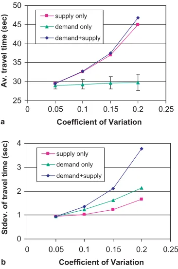
634 a single equilibrium state but continue to vary ad infinitum.Fig. 4 compares the relative impacts 635 of demand and supply variability on the averages and variances in daily vehicle travel times; the 636 comparison is made under the assumption that a demand variability range of 0 <bd< 0.2 is
com-637 parable to a supply variability range of 0 <bs+bv< 0.2. BothFigs. 3 and 4show that the
day-to-638 day total vehicle-hours are much higher on average at higher variability than at lower variability. 639 More specifically Fig. 4(a) shows that the demand variability on its own does not substantially 640 affect the averagetravel times, most of the increases being due to supply variability. However, 641 the demand variability introduce greatervariationin day-to-day travel times than does the supply 642 variability (Fig. 4(b)). This implies that a network becomes more unreliable as the demand vari-643 ation increases.
644 A further study was carried out on the network, withbd, bs, and bv all being set at 0.2 and a
[image:20.544.116.499.112.378.2]645 total of 1000 days being simulated.Fig. 5shows the frequency distribution of total network travel 646 times by day over the 1000 days simulated. It can be seen that the distribution is skewed towards 647 higher travel times, illustrating the existence of a small number of days with very high total travel 648 time. These days, although relatively few, have a significant impact on the average result since 649 they are not compensated by days with extremely small total travel time. Thus the mean travel 650 time of 98.6 is significantly greater than the mode of 88.7 and the median of 95.0.
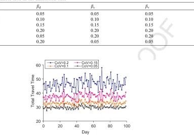
Table 1
Coefficient of variances used in the simulation tests
Test number bd bs bv
1 0.05 0.05 0.05
2 0.10 0.10 0.10
3 0.15 0.15 0.15
4 0.20 0.20 0.20
5 0.05 0.20 0.20
6 0.20 0.05 0.05
20 30 40 50 60
0 20 40 60 80 100
Day
Total Travel Time
CoV=0.2 CoV=0.15
CoV=0.1 CoV=0.05
UNCORRECTED
PROOF
25 30 35 40 45 50
0 0.05 0.1 0.15 0.2 0.25
Coefficient of Variation
Av. travel time (sec)
supply only
demand only
demand+supply
0 1 2 3 4
0 0.05 0.1 0.15 0.2 0.25
Coefficient of Variation
Stdev. of travel time (sec)
supply only
demand only
demand+supply a
b
Fig. 4. Average (a) and standard deviation (b) in daily travel times as a function of demand and supply variability.
Average Travel Time
160.0170.0180.0 190.0200.0 210.0 150.0
140.0 130.0 120.0 110.0 100.0 90.0 80.0 70.0
Frequency
200
175
150
125
100
75
50
25
[image:21.544.177.360.95.372.2]0
UNCORRECTED
PROOF
651 6.4. Responsive traffic signals
652 In this example, we apply the full model to a study of the effect of responsive signals on network 653 performance and driversÕroute choice. The model was tested on a small artificial network with 654 four possible routes, four signalised junctions and two O–D pairs (see Fig. 6).
655 The signals may be set by a simple responsive equi-saturationpolicy where the green
propor-656 tions allocated to each stage are determined based on the number of vehicles discharged in the 657 previous cycle. Here, signal cycles were kept constant and a minimum green period of 8 s was 658 maintained. In addition, a fixed plan optimised to the average traffic condition is used for com-659 parison. A total of 100 days and two levels of variability in daily demand (bd= 0.05 and 0.2) were
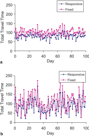
660 simulated. The averages and standard deviations in network total travel times (in vehicle-hours) 661 are summarised inTable 2. Day-to-day total vehicle-hours are shown inFig. 7(a) and (b) for the 662 low and high levels of variability respectively.
663 It can be seen that:
664 (a) Under both signal control policies, both the average and variance in vehicle-hours are higher
665 at higher demand variability. This conforms with the results found in Sections 6.2 and 6.3.
666 (b) Average travel times are lower under the responsive policy than under the fixed plan.
B
A C D E F
G
[image:22.544.157.402.331.493.2]H
Fig. 6. The network for testing the signal control policies. Intersections C, D, E and F are signalised and the two O–D pairs are A to B and B to A. One-way streets are indicated by arrows.
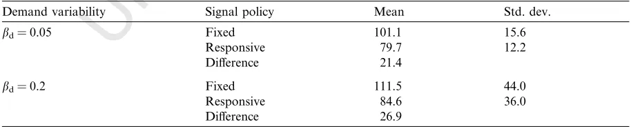
Table 2
Summary results of network total travel times (in vehicle-hours) under the two signal control policies
Demand variability Signal policy Mean Std. dev.
bd= 0.05 Fixed 101.1 15.6
Responsive 79.7 12.2
Difference 21.4
bd= 0.2 Fixed 111.5 44.0
Responsive 84.6 36.0
[image:22.544.46.503.568.660.2]UNCORRECTED
PROOF
667 (c) The responsive policy performed even better over the fixed signals under higher demand
var-668 iability; the average difference in travel times between the responsive signals and the fixed
669 plans is 26.7 s withbd= 0.2 compared with 20.4 s whenbd= 0.05 (Fig. 7).
670
671 The better travel performances produced by the responsive signals have also played an
impor-672 tant role in driversÕroute choice. Changes in signals were seen to attract drivers to the more direct 673 routes. With the responsive plans all drivers were assigned to the two minimum distance routes by 674 the end of 100 days, whereas with the fixed signal all four routes were used.
675 6.5. Scheme evaluation
676 In this example, we apply the full DRACULA model to a large, real-life network to examine
677 the short-term effect of a demand-management measure on driversÕroute choice and network
per-678 formance. The network covers a triangular area in the north of Leeds between the outer ring road 679 and the city centre (seeFig. 8). There are some 200 intersections, 400 links and 23,000 car trips per 680 hour in the morning peak period. The radial routes carrying most of the traffic to the city centre in 681 the morning are Kirkstall Road on the east, Meanwood Road on the west, and Otley Road and 682 Spen Lane in the middle.
0 50 100 150 200 250
0 20 40 60 80 100
Day
Total Travel Time
Responsive
Fixed
0 50 100 150 200 250
0 20 40 60 80 100
Day
Total Travel Time
Responsive Fixed a
[image:23.544.180.360.94.367.2]b
UNCORRECTED
PROOF
683 The proposed scheme introduces bus-only lanes on Otley Road inbound from the ring road to
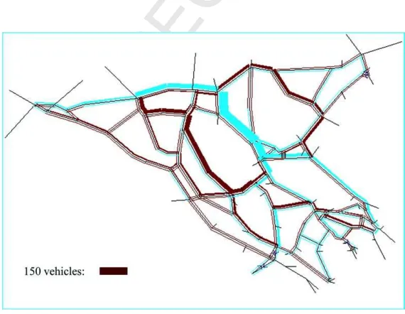
[image:24.544.131.416.90.299.2]684 Shaw Lane (shown as zigzag links inFig. 8). The road space available to general traffic is hence 685 reduced from two lanes to one. The remaining lane is further narrowed to reduce the free-flow 686 speed. The full DRACULA model is used to compare the route switching and travel time changes
Fig. 8. The North Leeds network. The proposed bus-lanes run along the links shown as zigzag lines. One-way streets are indicated by arrows.
[image:24.544.131.416.403.624.2]UNCORRECTED
PROOF
687 for the before-and-after scenarios. A total of 100 days were simulated withbd,bsandbvall being688 set to 0.1. Only the car trips were simulated. The first 50 days the network operates without the 689 capacity reduction on Otley Road. The bus lane was introduced on day 51 and was in operation 690 till the end of day 100.
691 With the severe reduction on road capacity along Otley Road, it is expected that some route
692 switching to alternative routes must take place. Fig. 9shows the differences in average link flows 693 between the 20-days before and 20-days after the introduction of the bus lane. It can be seen that 694 flow through the upper Otley Road was significantly lower after the introduction of the bus lane, 695 due to the reduction of road capacity on Otley Road. Much of those flows were diverted to nearby 696 Spen Lane or Meanwood Road. An analysis of trips from the top of Otley Road just outside the 697 Ring Road to the City Centre (an O–D pair whose minimum distance route is along Otley Road) 698 reveals that the average journey time has increased by 10% after the scheme was introduced.
699 7. Conclusions
700 Many papers have been written highlighting the potential advantages of microsimulation
ap-701 proaches over traditional static equilibrium models. However, to compete with the full function-702 ality of the equilibrium approach, especially in transport planning applications, we believe that it
703 is essential to have an integrated approach to modelling driversÕ medium-term travel decisions
704 (choice of route and departure time, based on prior travel experiences) and the short-term evolu-705 tion of traffic flow. Such an integrated approach has been described in this paper, where all deci-706 sions are treated at the microscopic level, and a consistent approach to supply and demand 707 modelling is utilised. We have subsequently demonstrated how such an approach may be used 708 to test complex measures and obtain forecasts that are beyond conventional equilibrium ap-709 proaches, such as predictions of policy impacts on the variability in travel times and flows.
710 By explicitly modelling variability at several levels the approach avoids the potential bias of
711 conventional models to over-estimate network performance as mentioned in Section 1. By work-712 ing at a disaggregate microsimulation level it deals naturally with time-dependent queues which 713 occur with junctions which are near or just over capacity. It can also deal with lane choice and 714 lane sharing problems whereby a single vehicle at the head of a lane which is turning to the offside 715 and is blocked by opposing traffic may therefore block that lane for straight ahead and/or near-716 side turns. By operating in real time it may be used to provide inputs to other real-time models 717 such as vehicle emission and dispersion models or noise models. Since these processes do not di-718 rectly affect driver behaviour they can be thought of as add-ons—albeit very important ones— 719 rather than integral components.
720 While a particular collection of assumptions, which we have referred to as DRACULA, has
UNCORRECTED
PROOF
728 1950s, it is only more recently that serious momentum has begun to test alternative theories729 against field data, beyond simple tests of aggregate consistency (Chakroborty and Kikuchi,
730 1999; Brackstone et al., 2002; Rakha and Crowther, 2003; Wu et al., 2003; Bham and Benekohal, 731 2004). We believe the continued study of field data to be one of the important priority areas for 732 future research in this area.
733 Acknowledgments
734 We wish to acknowledge a grant from the UK Engineering and Physical Science Research
735 Council and useful discussions with a large number of colleagues both at ITS and elsewhere over 736 a long period of time.
737 References
738 Adler, J.L., Satapathy, G., Manikonda, V., Bowles, B., Blue, V.J., 2005. A multi-agent approach to cooperative traffic
739 management and route guidance. Transportation Research B 39 (4), 297–318.
740 Alfa, A.S., Minh, D.L., 1979. A stochastic model for the temporal distribution of traffic demand—the peak hour
741 problem. Transportation Science 13, 315–324.
742 Algers, S., Bernauer, E., Boero, M., Breheret, L., Dougherty, M., Fox, K., Gabard, J.-F., 1997. Review of
743 microsimulation models. Delierable No. 3, SMARTEST Project, EU. Available from: <www.its.leeds.ac.uk/
744 projects/smartest/deliv3f.html>.
745 Akamatsu, T., 1996. Cyclic flows, Markov process and stochastic traffic assignment. Transportation Research 30B (5),
746 369–386.
747 Ambrosino, G., Sassoli, P., Bielli, M., Carotenuto, P., Romanazzo, M., 1999. A modeling framework for impact
748 assessment of urban transport systems. Transportation Research 4D, 39–73.
749 Barcelo´, J., Casas, J., 2004. Heuristic dynamic assignment based on AIMSUN microscopic traffic simulator. Paper
750 presented at the 5th Triennial Symposium on Transportation Analysis, Guadeloupe.
751 Ben-Akiva, M., De Palma, A., Kanaroglou, P., 1986. Dynamic model of peak period traffic congestion with elastic
752 arrival rates. Transportation Science 20 (2), 164–181.
753 Ben-Akiva, M., Cuneo, D., Hasan, M., Jha, M., Yang, Q., 2003. Evaluation of freeway control using a microscopic
754 simulation laboratory. Transportation Research 11C, 29–50.
755 Bham, G.H., Benekohal, R.F., 2004. A high fidelity traffic simulation model based on cellular automata and
car-756 following concepts. Transportation Research 12C, 1–32.
757 Bonsall, P., Liu, R., Young, W., in press. Modelling safety-related driving behaviour—impact of parameter values.
758 Transportation Research A.
759 Brackstone, M., Sultan, B., McDonald, M., 2002. Motorway driver behaviour: studies on car following. Transportation
760 Research 5F, 31–46.
761 Bullock, D., Johnson, B., Wells, R.B., Kyte, M., Li, Z., 2004. Hardware-in-the-loop simulation. Transportation
762 Research 12C, 73–89.
763 Cantarella, G.E., Cascetta, E., 1995. Dynamic process and equilibrium in transportation networks: towards a unifying
764 theory. Transportation Science 29 (4), 305–329.
765 Cascetta, E., 1989. A stochastic process approach to the analysis of temporal dynamics in transportation networks.
766 Transportation Research 23B, 1–17.
767 Chakroborty, P., Kikuchi, S., 1999. Evaluation of the General Motors based car-following models and a proposed
768 fuzzy inference model. Transportation Research 7C, 209–235.
769 Chang, T.-H., Lai, I.-S., 1997. Analysis of characteristic of mixed traffic flow of autopilot vehicles and manual vehicles.
UNCORRECTED
PROOF
771 Cova, T.J., Johnson, J.P., 2003. A network flow model for lane-based evacuation routing. Transportation Research772 37A, 579–604.
773 Davis, L.C., 2003. Modification of the optimal velocity traffic model to include delay due to driver reaction time.
774 Physica 319A, 557–567.
775 Dia, H., 2002. An agent-based approach to modelling driver route choice behaviour under the influence of real-time
776 information. Transportation Research 10C, 331–349.
777 Emmerink, R.H.M., Nijkamp, P. (Eds.), 1999. Behavioural and network impacts of driver information systems.
778 Avebury, Aldershot, UK.
779 Emmerink, R.H.M., Axhausen, K.W., Nijkamp, P., Rietveld, P., 1994. Effects of information in road transport
780 networks with recurrent congestion. Transportation 22, 21–53.
781 Eskafi, F., Khorramabadi, D., Varaiya, P., 1995. An automated highway system simulator. Transportation Research
782 3C (1), 1–17.
783 Fellendorf, M., Vortisch, P., 2000. Integrated modelling of transport demand, route choice, traffic flow and traffic
784 emissions. Paper presented at the 79th Annual Meeting of Transport Research Board, Washington, USA.
785 Gipps, P.G., 1981. A behavioural car-following model for computer simulation. Transportation Research 15B, 105–
786 111.
787 Hasan, M., Jha, M., Ben-Akiva, M., 2002. Evaluation of ramp control algorithms using microscopic traffic simulation.
788 Transportation Research 10C, 229–256.
789 Hazelton, M., Watling, D.P., in press. Computing equilibrium distributions for Markov traffic assignment models.
790 Transportation Science.
791 Hidas, P., 2002. Modelling lane changing and merging in microscopic traffic simulation. Transportation Research 10C,
792 351–371.
793 Hu, T.-Y., Mahmassani, H.S., 1997. Day-to-day evolution of network flows under real-time information and reactive
794 signal control. Transportation Research 5C (1), 51–69.
795 Huang, D., Huang, W., 2002. The influence of tollbooths on highway traffic. Physica 312A, 597–608.
796 Huijberts, H.J.C., 2002. Analysis of a continuous car-following model for a bus route: existence, stability and
797 bifurcations of synchronous motions. Physica 308A, 489–517.
798 Hunt, P.B., Robertson, D.I., Bretherton, R.D., Winton, R.I., 1981. SCOOT—a traffic responsive method of
799 coordinating signals. TRRL Laboratory Report 1014.
800 Institute of Transportation Engineers, 1982. Transportation and traffic engineering handbook, second ed.
Prentice-801 Hall, Englewood Cliffs, NJ.
802 Khan, S.I., Ritchie, S.G., 1998. Statistical and neural classifiers to detect traffic operational problems on urban arterials.
803 Transportation Research 6C, 291–314.
804 Kimber, R.M., 1989. Gap-acceptance and empiricism in capacity prediction. Transportation Science 23 (2), 100–111.
805 Ko¨ll, H., Bader, M., Axhausen, K.W., 2004. Driver behaviour during flashing green before amber: a comparative study.
806 Accident Analysis and Prevention 36, 273–280.
807 Kosonen, I., 2003. Multi-agent signal control based on real-time simulation. Transportation Research 11C, 389–403.
808 Laird, J., Druitt, S., Fraser, D., 1999. Edinburgh city centre: a microsimulation case-study. TEC 40 (2), 72–76.
809 Lee, J.-K., Lee, J.-J., 1997. Discrete event modeling and simulation for flow control in an automated highway system.
810 Transportation Research 5C (3/4), 179–195.
811 Liu, R., 2005. The DRACULA microscopic traffic simulation model. In: Kitamura, R., Kuwahara, M. (Eds.),
812 Transport simulation. Springer.
813 Liu, R., Tate, J., 2004. Network effects of intelligent speed adaptation systems. Transportation 31 (3), 297–325.
814 Liu, R., van Vliet, D., Watling, D.P., 1995. DRACULA: Dynamic Route Assignment Combining User Learning and
815 microsimulAtion. In: Proc. PTRC Annual Conference, Seminar E, pp. 143–152.
816 Liu, R., Clark, S.D., Montgomery, F.O., Watling, D.P., 1999. Microscopic modelling of traffic management measures
817 for guided bus operationSelected Proceedings of 8th World Conference on Transport Research, vol. 2. Elsevier, pp.
818 367–380.
819 Liu, R., Silva, J., Seco, A., submitted for publication. A bi-modal microsimulation tool for assessment of pedestrian